


Forecasting Stock Using Deep Learning Along With Indicators
Forecasting Stock Using Deep Learning Along With Indicators
Today I am going to show you how to prediction stock prices using deep learning. Also add indicators like sell and buy on chart.

Steps involved:
Baseline Model
ARIMA
Sentiment Analysis
Feature Selection with XGBoost
Deep Neural Network
Pattern Recognition by Hand
Q-Learning
Import Libraries
import os
import pandas as pd
import matplotlib.pyplot as plt
import matplotlib.patches as patches
import seaborn as sns
import warnings
import numpy as np
from numpy import array
from importlib import reload # to reload modules if we made changes to them without restarting kernel
from sklearn.naive_bayes import GaussianNB
from xgboost import XGBClassifier # for features importance
warnings.filterwarnings('ignore')
plt.rcParams['figure.dpi'] = 227 # native screen dpi for my computerFirst of all we are going to import various libraries such as os, pandas, matplotlib, seaborn, warnings, numpy and other important libraries. It filters out warning messages, set the DPI of matplotlib, for more clearer plots.
import statsmodels.api as sm
from statsmodels.tsa.arima_model import ARIMA
from statsmodels.tsa.statespace.sarimax import SARIMAX
from statsmodels.graphics.tsaplots import plot_pacf, plot_acf
from sklearn.metrics import mean_squared_error, confusion_matrix, f1_score, accuracy_score
from pandas.plotting import autocorrelation_plot
This code imports a bunch of stuff from different libraries to help us predict stock prices using machine learning. The statsmodels library has all sorts of tools for time series analysis and modeling, including ARIMA and SARIMAX models. We can use functions like plot_pacf and plot_acf to plot autocorrelation and partial autocorrelation plots, which can help us understand how the data is correlated with itself over time. The scikit-learn library has functions for evaluating our model’s performance, like mean squared error, confusion matrix, f1 score, and accuracy score. And the pandas.plotting library can help us plot autocorrelation plots for our data.
import tensorflow.keras as keras
from tensorflow.python.keras.optimizer_v2 import rmsprop
from functools import partial
from tensorflow.keras import optimizers
from tensorflow.keras.models import Sequential, Model
from tensorflow.keras.layers import Input, Flatten, TimeDistributed, LSTM, Dense, Bidirectional, Dropout, ConvLSTM2D, Conv1D, GlobalMaxPooling1D, MaxPooling1D, Convolution1D, BatchNormalization, LeakyReLU
from bayes_opt import BayesianOptimization
from tensorflow.keras.utils import plot_modelThis code imports all the libraries and functions we need to predict stock prices using machine learning and Bayesian optimization. We’re using TensorFlow Keras for our machine learning model, and Bayesian optimization to help us tune the model’s hyperparameters.
import functions
import plotting
This code imports two custom modules: functions and plotting. These modules were likely written specifically for this stock prediction project.
The functions module contains functions that do all sorts of things related to stock prediction, like cleaning the data, creating new features, training models, and evaluating models.
The plotting module contains functions that make it easy to visualize the results of the stock prediction, like plotting the actual stock prices vs. the predicted values, or showing how different models performed.
By importing these modules, the code can access all the functionality they provide and use it for its stock prediction task.
np.random.seed(66)This line of code tells the numpy library to use the number 66 as its random seed. This means that every time the program is run, it will generate the same sequence of random numbers.
This is useful for machine learning because it allows us to get consistent results each time we run our program. This is important because it allows us to compare different models and algorithms fairly, and to make sure that our results are reliable.
Loading Data
Reading stock datas:
files = os.listdir('data/stocks')
stocks = {}
for file in files:
    if file.split('.')[1] == 'csv':
        name = file.split('.')[0]
        stocks[name] = pd.read_csv('data/stocks/'+file, index_col='Date')
        stocks[name].index = pd.to_datetime(stocks[name].index)
This code is for predicting stock prices using machine learning. It starts by looking at all the CSV files in a directory called data/stocks.
Next, it creates a dictionary called stocks. This dictionary will store all of the stock data, with the name of the stock as the key.
Then, it loops through all of the CSV files in the directory. For each file, it checks to see if it has a .csv extension. If it does, then the code reads the file into a Pandas DataFrame.
When reading the CSV file, the code specifies that the Date column should be used as the index. This means that the Date column will be used to sort the data and to identify each row of data.
Finally, the code converts the Date column to datetime format. This ensures that the dates are formatted correctly for further analysis.
Once the code has finished looping through all of the CSV files, the stocks dictionary will contain all of the stock data, with the name of the stock as the key and the stock data as the value.
Baseline Model
def baseline_model(stock): baseline_predictions = np.random.randint(0, 2, len(stock))
accuracy = accuracy_score(functions.binary(stock), baseline_predictions)
return accuracyNow in this code we define a function known as baseline_model() that takes in a series or array of stock data and returns the accuracy of a baseline prediction model.
The baseline prediction model is simply a model that predicts that the stock price will go up or down with a 50% chance. To implement this model, the code generates a series of random numbers between 0 and 1, with the same length as the input stock data. These random numbers are then compared with the true values of the stock data using a binary classification approach.
In binary classification, each data point is assigned to one of two classes. In this case, the two classes are “up” and “down.” To classify a data point, the code compares the random number generated for the data point to a threshold value. If the random number is greater than the threshold value, then the data point is classified as “up.” Otherwise, the data point is classified as “down.”
The accuracy of the baseline prediction model is calculated using the accuracy_score() function. This function takes in two arrays of predictions and labels and returns the percentage of predictions that were correct.
The code uses the NumPy library for generating random numbers and the functions.binary() function to convert the input stock data into a binary format.
baseline_accuracy = baseline_model(stocks['tsla'].Return)
print('Baseline model accuracy: {:.1f}%'.format(baseline_accuracy * 100))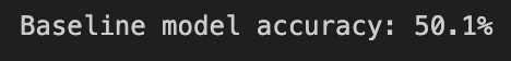
It passes the returns data of the TSLA stock to the baseline_model() function, which we defined earlier. The function returns the accuracy of the model, which is then stored in the variable baseline_accuracy. The next line prints the accuracy in percentage format.
The baseline_model() function is a simple model that predicts that the stock price will go up or down with a 50% chance. So, the baseline accuracy is essentially the percentage of times that the model would have correctly predicted the direction of the stock price.
Accuracy Distribution
base_preds = []
for i in range(1000):
    base_preds.append(baseline_model(stocks['tsla'].Return))

plt.figure(figsize=(16,6))
plt.style.use('seaborn-whitegrid')
plt.hist(base_preds, bins=50, facecolor='#4ac2fb')
plt.title('Baseline Model Accuracy', fontSize=15)
plt.axvline(np.array(base_preds).mean(), c='k', ls='--', lw=2)
plt.show()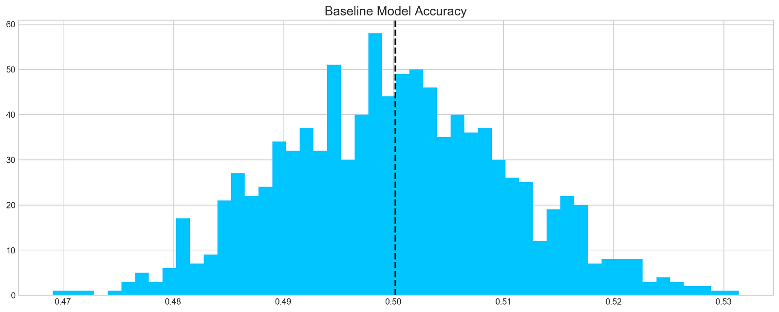
This code snippet starts by initializing an empty list called base_preds. Then, it runs a loop 1000 times and calls a function called baseline_model() with the argument stocks[‘tsla’].Return for each iteration. The return value of the function call is appended to the base_preds list.
The baseline_model() function is a simple model that predicts that the stock price will go up or down with a 50% chance. So, the base_preds array will contain 1000 predictions of whether the stock price will go up or down.
After the loop, the code creates a figure with a size of 16x6 using Matplotlib. It sets the style to “seaborn-whitegrid” and creates a histogram using the data in the base_preds list. The histogram has 50 bins and uses the color ‘#4ac2fb’.
The code then adds a title “Baseline Model Accuracy” to the plot with a font size of 15. It also adds a vertical line at the mean value of the base_preds array, using a black color and a dashed line style. Finally, the plot is displayed.
This code snippet provides a way to visualize the accuracy of the baseline model. The histogram shows how many predictions were made for each accuracy level. The vertical line shows the average accuracy of the model.
ARIMA
print('Tesla historical data contains {} entries'.format(stocks['tsla'].shape[0]))
stocks['tsla'][['Return']].head()
This code prints the number of entries in the historical data of Tesla stocks. It uses the format() function to insert the value of the number of entries into the print statement. The next line of code retrieves the first few rows of the Return column from the historical data of Tesla stocks and displays them.
In other words, this code tells us how many Tesla stock prices are in the data set, and then shows us the first few rows of the data set so we can get a sense of what it looks like.
Autocorrelation
plt.rcParams['figure.figsize'] = (16, 3)
plot_acf(stocks['tsla'].Return, lags=range(300))
plt.show()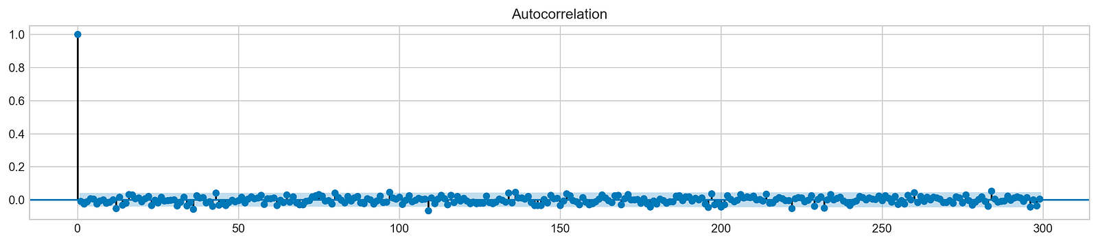
This code plots the autocorrelation function (ACF) of the returns of Tesla stock using Matplotlib. The ACF measures how correlated a stock’s returns are with its past returns at different time lags. The plot shows how this correlation changes over time, for up to 299 days.
The ACF can be used to analyze historical stock returns to identify patterns in the stock’s price movements. For example, a positive ACF at a lag of 1 day suggests that the stock is more likely to go up if it has gone up in the previous day. This information could be used to develop a trading strategy.
orders = [(0,0,0),(1,0,0),(0,1,0),(0,0,1),(1,1,0)]train = list(stocks['tsla']['Return'][1000:1900].values)
test = list(stocks['tsla']['Return'][1900:2300].values)all_predictions = {}for order in orders:
try:
history = train.copy()
order_predictions = []
for i in range(len(test)):
model = ARIMA(history, order=order) # defining ARIMA model
model_fit = model.fit(disp=0) # fitting model
y_hat = model_fit.forecast() # predicting 'return'
order_predictions.append(y_hat[0][0]) # first element ([0][0]) is a prediction
history.append(test[i]) # simply adding following day 'return' value to the model
print('Prediction: {} of {}'.format(i+1,len(test)), end='\r')
accuracy = accuracy_score(
functions.binary(test),
functions.binary(order_predictions)
)
print(' ', end='\r')
print('{} - {:.1f}% accuracy'.format(order, round(accuracy, 3)*100), end='\n')
all_predictions[order] = order_predictions
except:
print(order, '<== Wrong Order', end='\n')
pass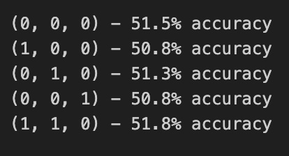
This code is using machine learning to predict stock prices. It does this by trying out different configurations for an ARIMA model.
First, the code defines a list of orders. Each order represents a different configuration for the ARIMA model. Then, the code splits the stock data into two sets: a training set and a testing set.
Next, the code iterates over each order in the list. For each order, the code tries to fit an ARIMA model to the training data. If the model is fitted successfully, the code uses the model to make predictions for the testing data. The predictions are stored in a list.
After making predictions for all test data, the code calculates the accuracy of the predictions by comparing them to the actual values. The accuracy is printed to the console.
If an order fails to be processed, which could be due to an incorrect configuration, the code displays an error message.
Finally, the code stores all the predictions in a dictionary.
Review Predictions
fig = plt.figure(figsize=(16,4))
plt.plot(test, label='Test', color='#4ac2fb')
plt.plot(all_predictions[(0,1,0)], label='Predictions', color='#ff4e97')
plt.legend(frameon=True, loc=1, ncol=1, fontsize=10, borderpad=.6)
plt.title('Arima Predictions', fontSize=15)
plt.xlabel('Days', fontSize=13)
plt.ylabel('Returns', fontSize=13)
plt.annotate('',
xy=(15, 0.05),
xytext=(150, .2),
fontsize=10,
arrowprops={'width':0.4,'headwidth':7,'color':'#333333'}
)
ax = fig.add_subplot(1, 1, 1)
rect = patches.Rectangle((0,-.05), 30, .1, ls='--', lw=2, facecolor='y', edgecolor='k', alpha=.5)
ax.add_patch(rect)plt.axes([.25, 1, .2, .5])
plt.plot(test[:30], color='#4ac2fb')
plt.plot(all_predictions[(0,1,0)][:30], color='#ff4e97')
plt.tick_params(axis='both', labelbottom=False, labelleft=False)
plt.title('Lag')
plt.show()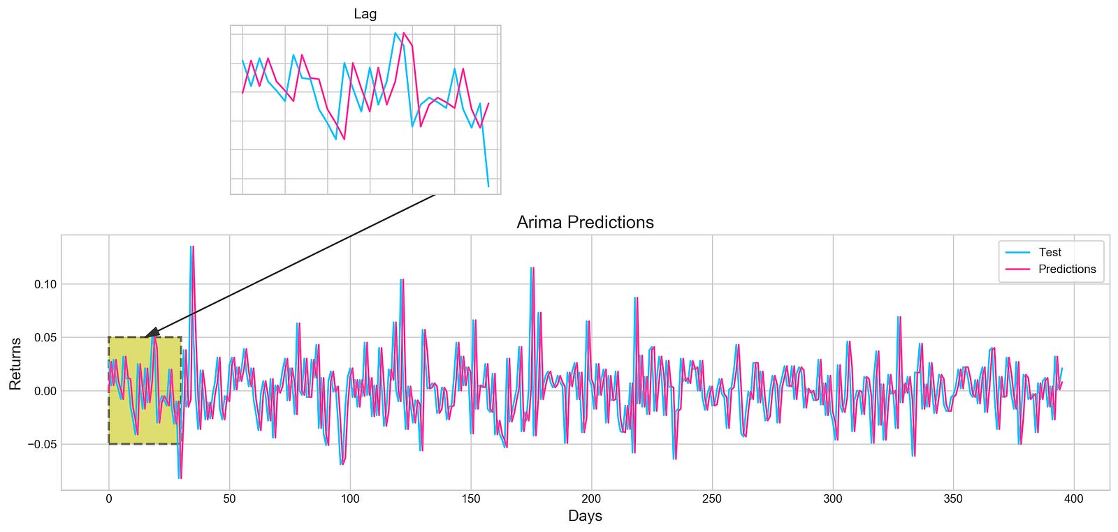
This code plots a graph of the actual and predicted stock prices for a given period of time. It uses Matplotlib to create a figure with a specific size, and then plots the test data and the predictions on the graph using different line styles and colors. Legends are added to the graph to identify the different lines, and a title and labels are also added to make the graph more informative.
The code also includes an annotation arrow on the graph to indicate a specific point. This can be used to highlight an important point in the data or to show a trend. Additionally, the code adds a rectangle patch to highlight a specific region on the graph. This can be used to focus on a particular part of the data or to show a specific pattern.
In addition to the main plot, the code also creates a smaller subplot within the main plot. This subplot shows a zoomed-in view of the test and predicted data for the first 30 days. The subplot has no axis labels and is titled “Lag”. This allows us to see the data in more detail and identify any trends or patterns that may be less obvious in the main plot.
Histogram
plt.figure(figsize=(16,5))
plt.hist(stocks['tsla'][1900:2300].reset_index().Return, bins=20, label='True', facecolor='#4ac2fb')
plt.hist(all_predictions[(0,1,0)], bins=20, label='Predicted', facecolor='#ff4e97', alpha=.7)
plt.axvline(0, c='k', ls='--')
plt.title('ARIMA True vs Predicted Values Distribution', fontSize=15)
plt.legend(frameon=True, loc=1, ncol=1, fontsize=10, borderpad=.6)
plt.show()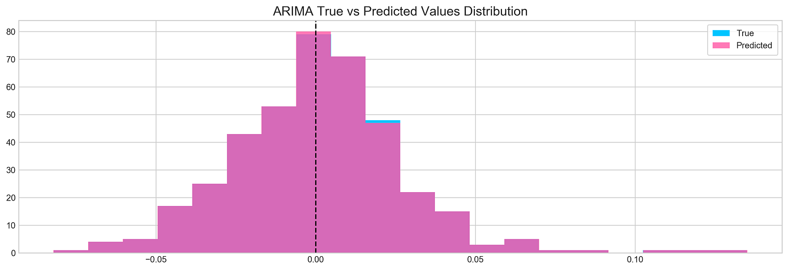
This code creates a histogram plot that compares the distribution of the actual and predicted stock returns for Tesla stock. The data used for the histogram is a subset of the Tesla stock returns from index 1900 to 2300. The actual stock returns are plotted in blue, while the predicted stock returns are plotted in pink with some transparency. A vertical dashed line at 0 is also plotted.
This code can be used to evaluate the performance of an ARIMA model for stock prediction. By comparing the distribution of the actual and predicted values, we can see how well the model is able to capture the overall trend of the stock market, as well as any short-term fluctuations.
For example, if the distribution of the predicted values is very similar to the distribution of the actual values, then this suggests that the model is doing a good job of predicting the stock market. However, if the distribution of the predicted values is significantly different from the distribution of the actual values, then this suggests that the model is not doing a good job of predicting the stock market.
Sentiment Analysis
tesla_headlines = pd.read_csv('data/tesla_headlines.csv', index_col='Date')This code uses the Pandas library to read a CSV file called “tesla_headlines.csv”. The file contains headlines related to the stock market performance of the company Tesla. The “index_col” parameter is set to “Date”, which means that the “Date” column in the CSV file will be used as the index for the resulting Pandas DataFrame.
A DataFrame is a data structure that is similar to a spreadsheet, with rows and columns. The index of a DataFrame is a unique identifier for each row. In this case, the “Date” column is being used as the index, which means that each row in the DataFrame will be uniquely identified by its date.
This code is useful for reading CSV data into Pandas DataFrames. DataFrames are a powerful data structure for data manipulation and analysis. For example, we can use DataFrames to filter the data, calculate statistics, and create visualizations.
tesla = stocks['tsla'].join(tesla_headlines.groupby('Date').mean().Sentiment)This code combines the stock data for Tesla with the average sentiment for each date from a dataset called “tesla_headlines”. The resulting data frame, stored in the variable tesla, can be used for stock prediction using machine learning techniques.
Sentiment analysis is a technique for extracting the sentiment of a piece of text, such as whether it is positive, negative, or neutral. In this case, the code is using sentiment analysis to extract the average sentiment of news headlines related to Tesla.
Combining the stock data with the sentiment data can provide valuable insights into how news headlines may be impacting Tesla’s stock price. For example, if there is a sudden increase in negative sentiment, it is possible that this could lead to a decrease in Tesla’s stock price.
Machine learning algorithms can be trained on the combined stock and sentiment data to learn to predict future stock prices. By taking into account the sentiment of news headlines, machine learning algorithms can potentially improve their ability to predict stock prices.
tesla.fillna(0, inplace=True)This code is a part of stock prediction using machine learning, specifically for Tesla stock. The fillna() function is being used to replace any missing values in the tesla data frame with the number 0. The inplace=True parameter ensures that the changes are made directly to the tesla data frame without creating a new object.
Missing values are a common problem in data sets, and they can interfere with machine learning algorithms. The fillna() function can be used to replace missing values with a variety of different values, such as the mean, median, or mode of the data set. In this case, the tesla data frame is being filled in with the number 0, which is a common choice for filling in missing values in stock data.
The inplace=True parameter tells the fillna() function to make the changes directly to the tesla data frame. This is more efficient than creating a new data frame, and it saves memory.
plt.style.use('seaborn-whitegrid')
plt.figure(figsize=(16,6))
plt.plot(tesla.loc['2019-01-10':'2019-09-05'].Sentiment.shift(1), c='#3588cf', label='News Sentiment')
plt.plot(tesla.loc['2019-01-10':'2019-09-05'].Return, c='#ff4e97', label='Return')
plt.legend(frameon=True, fancybox=True, framealpha=.9, loc=1)
plt.title('Tesla News Sentiment and Daily Return', fontSize=15)
plt.show()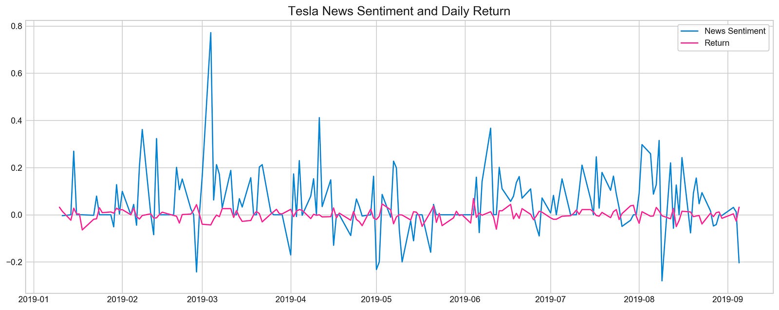
This code creates a line plot that compares the sentiment of news about Tesla stock to the daily return of the stock. The plot shows how the sentiment of news about Tesla stock changes over time, and how this relates to the daily return of the stock.
The code uses the seaborn-whitegrid style and sets the figure size to 16x6. This means that the plot will have a white background with a grid, and it will be 16 inches wide by 6 inches tall.
The plot shows the sentiment data from the 2019–01–10 to 2019–09–05 shifted by one day. This means that the sentiment data for each day is shown on the plot for the following day. This is done to account for the fact that news sentiment can take some time to impact the stock market.
The plot also shows the daily return data for the same period. The daily return is the percentage change in the stock price from one day to the next.
The plot includes a legend to identify the two lines, and a title to explain what the plot shows. The plot is then displayed using the plt.show() function.
pd.DataFrame({
    'Sentiment': tesla.loc['2019-01-10':'2019-09-05'].Sentiment.shift(1),
    'Return': tesla.loc['2019-01-10':'2019-09-05'].Return}).corr()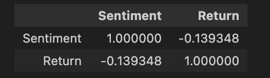
The code creates a Pandas DataFrame that computes the correlation between the Sentiment and Return columns for Tesla stock. The Sentiment column is created by shifting the original Sentiment column by one index, which means that the sentiment data for each day is shown on the plot for the following day. This is done to account for the fact that news sentiment can take some time to impact the stock market.
The Return column is created by selecting the Return column of the tesla dataset within a specified date range. The correlation between these two columns is then calculated using the corr() function.
The correlation coefficient is a measure of the strength and direction of the relationship between two variables. A correlation coefficient of 1 indicates a perfect positive correlation, while a correlation coefficient of -1 indicates a perfect negative correlation. A correlation coefficient of 0 indicates no correlation.
In the context of this code, the correlation coefficient between the Sentiment and Return columns will indicate the strength and direction of the relationship between news sentiment and stock returns for Tesla stock. A positive correlation coefficient would suggest that positive news sentiment tends to be associated with positive stock returns, while a negative correlation coefficient would suggest that negative news sentiment tends to be associated with negative stock returns.
Feature Selection With XGBoost
scaled_tsla = functions.scale(stocks['tsla'], scale=(0,1))This code scales the Tesla stock data to a range of 0 to 1. This is done using the scale() function from the functions module.
Scaling is a common technique used in machine learning to prepare data for training and prediction. Scaling helps to ensure that all of the features in the data have a similar scale, which can improve the performance of machine learning algorithms.
There are many different scaling functions that can be used, but the scale() function is a simple and effective choice for many applications. It works by subtracting the mean of the data from each value and then dividing by the standard deviation.
The resulting scaled data is stored in the variable scaled_tsla. This scaled data can then be used for machine learning tasks, such as training a model to predict Tesla stock prices.
X = scaled_tsla[:-1]
y = stocks['tsla'].Return.shift(-1)[:-1]
This code first creates a new variable called X by selecting a subset of the scaled_tsla data, but discarding the last item in the dataset. It then creates a new variable called y by selecting the Return column from the tsla stocks dataframe, shifting the values by -1, and dropping the last item from the resulting series.
The scaled_tsla data is a scaled version of the Tesla stock data, and the y variable contains the Tesla stock returns, shifted by -1. This means that the y variable contains the Tesla stock returns for the next day, given the Tesla stock data for the current day.
This code is preparing the X and y variables for machine learning. The X variable will be used as the input to the machine learning algorithm, and the y variable will be used as the target variable. The machine learning algorithm will be trained to learn the relationship between the X variables and the y variable.
Once the machine learning algorithm is trained, it can be used to predict Tesla stock returns for the next day. This information can then be used to make informed investment decisions.
xgb = XGBClassifier()
xgb.fit(X[1500:], y[1500:])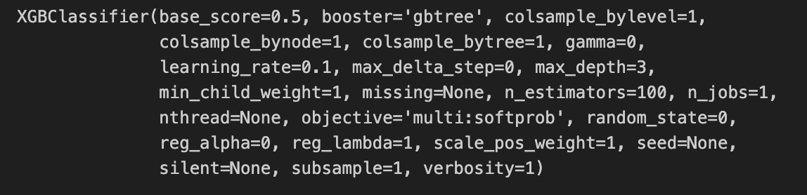
The code creates an instance of the XGBClassifier class, which is a machine learning algorithm used for classification. The fit() method is then called on the XGBClassifier instance, passing in a subset of the input data X and corresponding labels y. This fit() method trains the classifier on the provided data, allowing it to learn patterns and make predictions.
The XGBClassifier algorithm is a type of gradient boosting algorithm, which is a machine learning technique that combines the predictions of multiple weak learners to produce a strong learner. Gradient boosting algorithms are known for their ability to handle complex data and achieve high accuracy on a variety of machine learning tasks, including classification and regression.
The fit() method is a critical step in the machine learning process. It is during this step that the classifier learns the relationship between the input data X and the output labels y. Once the classifier is trained, it can be used to make predictions on new data.
The XGBClassifier algorithm is a powerful tool for machine learning. It can be used to solve a wide variety of classification problems, including spam filtering, fraud detection, and medical diagnosis.
Deep Neural Networks
n_steps = 21
scaled_tsla = functions.scale(stocks['tsla'], scale=(0,1))
X_train, \
y_train, \
X_test, \
y_test = functions.split_sequences(
scaled_tsla.to_numpy()[:-1],
stocks['tsla'].Return.shift(-1).to_numpy()[:-1],
n_steps,
split=True,
ratio=0.8
)The code defines a variable n_steps as 21, which represents the number of previous days of stock data that will be used to predict the next day’s stock price.
The code then scales the tsla column from the stocks dataframe using the scale function. This is done to ensure that all of the features in the data have a similar scale, which can improve the performance of machine learning algorithms.
The scaled tsla data is then used to split sequences into training and testing sets. The training set, denoted as X_train and y_train, is created by taking the scaled tsla data (excluding the last element) and the shifted Return values from the stocks dataframe (excluding the last element) using the split_sequences function. The last argument of split_sequences is set to split=True and a ratio of 0.8, indicating that the sequences should be split into training and testing sets with a ratio of 80% for training.
The testing set, denoted as X_test and y_test, is created similarly, but using the remaining 20% of the data.
Overall, this code prepares the data for stock prediction using machine learning by scaling the input data and splitting it into training and testing sets. The training set will be used to train the machine learning model, and the testing set will be used to evaluate the performance of the model.
LSTM Network
keras.backend.clear_session()n_steps = X_train.shape[1]
n_features = X_train.shape[2]model = Sequential()
model.add(LSTM(100, activation='relu', return_sequences=True, input_shape=(n_steps, n_features)))
model.add(LSTM(50, activation='relu', return_sequences=False))
model.add(Dense(10))
model.add(Dense(1))
model.compile(optimizer='adam', loss='mse', metrics=['mae'])The code is implementing a stock prediction model using machine learning using Keras.
The first step in the code is to clear the Keras session. This is done to ensure that there are no conflicting variables or models from previous training sessions.
Next, the code defines the number of time steps and features in the training data. The number of time steps is the number of previous days of stock data that will be used to predict the next day’s stock price. The number of features is the number of input variables that will be used to predict the next day’s stock price.
After this, the code creates a Sequential model. A Sequential model is a linear stack of layers. The model architecture consists of two LSTM (Long Short-Term Memory) layers.
LSTM layers are a type of recurrent neural network (RNN) that are well-suited for time series forecasting tasks. LSTM layers are able to learn long-term dependencies in the data, which is important for stock prediction.
The first LSTM layer in the model has 100 units and uses the ReLU activation function. It returns sequences of outputs. The input shape is determined by the number of time steps and features.
The second LSTM layer in the model has 50 units and also uses the ReLU activation function. It does not return sequences of outputs.
After the LSTM layers, there are two Dense layers. Dense layers are a type of fully connected neural network layer. The first Dense layer in the model has 10 units. The second Dense layer has 1 unit.
The second Dense layer outputs the prediction for the next day’s stock price.
The model is compiled using the Adam optimizer, mean squared error (mse) as the loss function, and mean absolute error (mae) as the metric.
The Adam optimizer is a popular optimizer for training machine learning models. It is known for its ability to converge quickly to good solutions.
Mean squared error (mse) is a common loss function for regression tasks. It measures the average squared difference between the predicted values and the actual values.
Mean absolute error (mae) is another common loss function for regression tasks. It measures the average absolute difference between the predicted values and the actual values.
Once the model is compiled, it can be trained on the training data. After the model is trained, it can be used to make predictions on new data.
model.summary()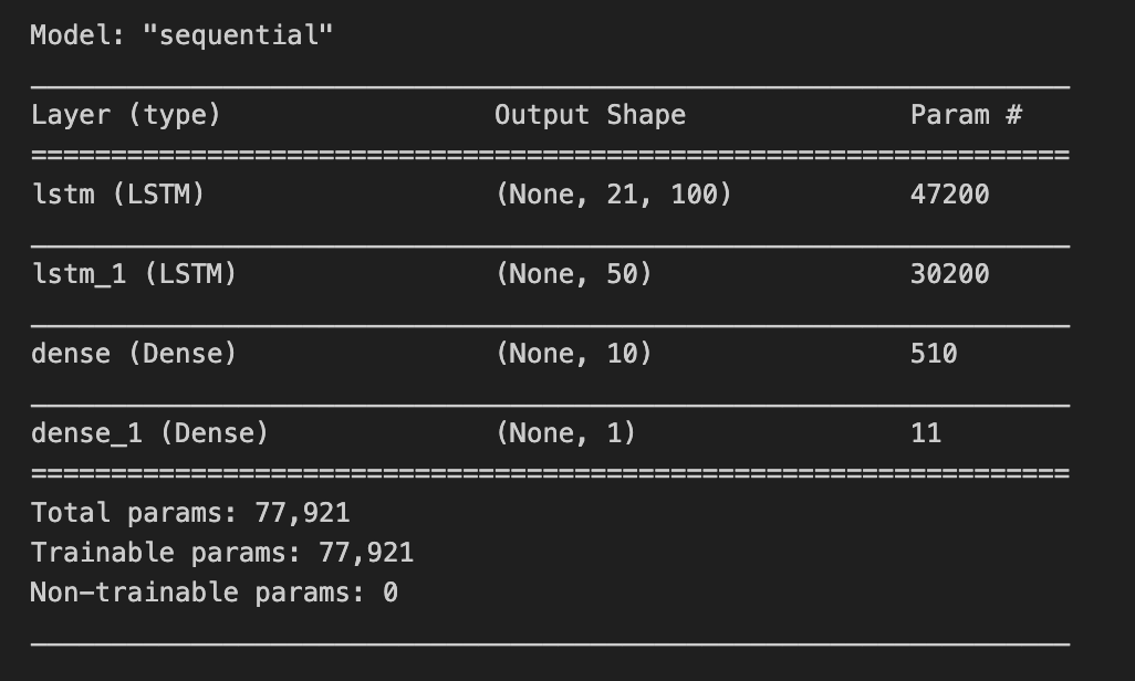
The model.summary() function in Keras is used to generate a summary of a machine learning model. This summary provides a lot of useful information about the model, including:
The name and type of each layer in the model
The number of parameters in each layer
The total number of trainable parameters in the model
The shape of the input and output tensors for each layer
This information can be used to understand the structure and complexity of the model, and it can help in troubleshooting and optimizing the model during the development process.
For example, the model.summary() function can be used to identify the layers in the model that have the most parameters. This information can be used to decide which layers to prune or regularize in order to reduce the risk of overfitting.
The model.summary() function can also be used to identify the layers in the model that have the largest input or output tensors. This information can be used to optimize the memory usage of the model and to improve the performance of the model on hardware with limited memory.
model.fit(X_train, y_train, epochs=100, verbose=0, validation_data=[X_test, y_test], use_multiprocessing=True)plt.figure(figsize=(16,4))
plt.plot(model.history.history['loss'], label='Loss')
plt.plot(model.history.history['val_loss'], label='Val Loss')
plt.legend(loc=1)
plt.title('LSTM - Training Process')
plt.show()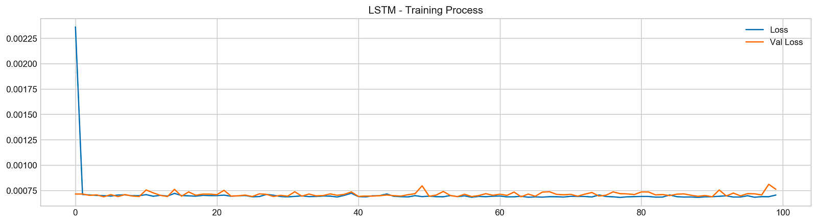
The code is fitting a machine learning model to X_train and y_train data for 100 epochs. It is using the X_test and y_test data for validation during the training process. The use_multiprocessing flag indicates that multiprocessing should be used during training. After training the model, the code plots the loss and validation loss values over the training process.
Epochs: An epoch is a single iteration over the entire training dataset. During each epoch, the model is trained on all of the training data.
Validation: Validation is the process of evaluating the performance of a machine learning model on a dataset that it has not been trained on. This helps to ensure that the model is not overfitting to the training data.
Multiprocessing: Multiprocessing is a technique that allows multiple processes to run simultaneously. This can improve the performance of machine learning algorithms, especially when training on large datasets.
Loss: The loss value is a measure of the difference between the predicted and actual values during training. The goal of training a machine learning model is to minimize the loss value.
Validation loss: The validation loss value is a measure of the difference between the predicted and actual values during validation.
Plotting the loss and validation loss values: Plotting the loss and validation loss values over the training process is a good way to visualize how the model is performing. If the loss and validation loss values are decreasing over time, then the model is learning. If the loss and validation loss values are increasing over time, then the model is not learning and may be overfitting to the training data.
pred, y_true, y_pred = functions.evaluation(
                    X_test, y_test, model, random=False, n_preds=50,
                    show_graph=True)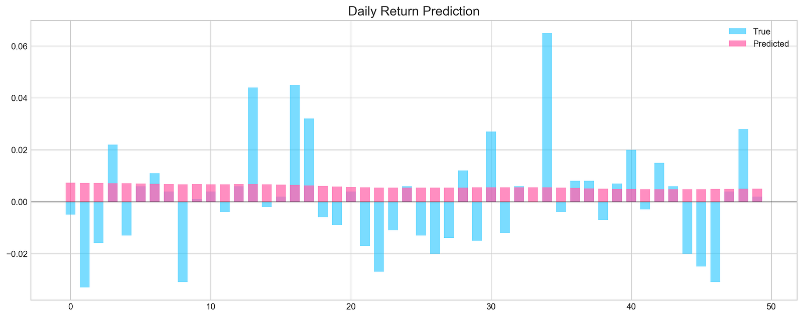
The X_test and y_test variables are the test data, which consist of features and corresponding target values, respectively. The model variable represents the machine learning model that has been trained on historical stock data.
The functions.evaluation() function is called to evaluate the model’s performance. It takes several arguments:
X_test: The test data features.
y_test: The test data target values.
model: The trained machine learning model.
random: A boolean parameter indicating whether to use random predictions or not. If random is set to True, then the function will generate random predictions for the target variable. Otherwise, the function will use the model to generate predictions for the target variable.
n_preds: The number of predictions to make.
The functions.evaluation() function returns three values:
pred: The predicted values of the target variable.
y_true: The true values of the target variable from the test data.
y_pred: The predicted values of the target variable based on the model’s predictions.
Additionally, the functions.evaluation() function also plots a graph to visualize the actual and predicted values of the target variable, if the show_graph parameter is set to True.