


Forecasting time series using multilayer perceptron models
Time series forecasting can be achieved using multilayer perceptrons.

MLPs are helpful for forecasting time series, but preparing the data can be challenging. A feature vector must be constructed using lag observations.
During this tutorial, you will learn how to forecast time series using a range of standard forecasting methods.
The purpose of this tutorial is to provide standalone examples of each type of model for each type of time series forecasting problem so you can copy and adapt them.
You will learn how to develop Multilayer Perceptron models for standard time series forecasting problems.
You will know the following after completing this tutorial:
Univariate time series forecasting using MLP models.
Modeling multivariate time series for multivariate forecasting.
Multi-step time series forecasting using MLP models.
Overview of the tutorial
Four parts make up this tutorial. They are as follows:
Models with univariate MLPs
MLP models with multivariate variables
MLP models with multiple steps
Models based on multivariate multi-step MLPs
MLP models with univariate coefficients
In univariate time series forecasting, Multilayer Perceptrons, or MLPs, can be used.
Time series with a single series of observations with a temporal ordering require a model to predict the next value based on the series of past observations.
The following two sections are divided into two parts:
Preparation of data
Model MLP
Preparation of data
An univariate series must be prepared before it can be modeled.
As input to the MLP model, a series of previous observations are mapped into an output observation. Therefore, the model must be able to learn from multiple examples, from the sequence of observations.
The following is an example of a univariate sequence:

A one-step prediction can be learned using three time steps as input and one time step as output for a sequence of input/output patterns called samples.

With split_sequence(), a univariate sequence will be split into multiple samples. The output will be a single time step for each sample.

On our small contrived dataset above, we can demonstrate this function.
Listed below is the full example.

Taking the example as an example, you will divide the univariate series into six samples, each with three input and output time steps.

The MLP model can learn how to map inputs and outputs based on the univariate series that we prepared earlier.
Model MLP
There is a hidden layer of nodes, and an output layer used for prediction in a simple MLP model.
For univariate time series forecasting, we can define an MLP as follows.
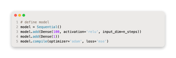
For the definition, it is important to determine the shape of the input; that is, how many steps are expected for each sample.
As an argument to split_sequence(), we provide the number of time steps we chose when preparing our dataset.
On the definition of first hidden layer, input_dim specifies the input dimension for each sample. In technical terms, each time step will be viewed as a separate feature, not as a separate time step.
The input data component for training data will almost always have these dimensions or shapes since there are usually multiple samples.

As we saw in the previous section, our split_sequence() function outputs the X with the shape [samples, features] ready for modeling.
Adam stochastic gradient descent is used to fit the model, and the loss function using the mean square error, or mSE, is used to optimize the model.
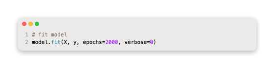
We can then fit the model on the training dataset once the model is defined.
Predictions can be made after the model has been fitted.
The following inputs can be used to predict the next value:

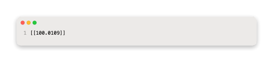
The model is expected to predict something like:

For the model to predict anything from one sample and three time steps, we must transform the input shape into two dimensions with [features, samples], for example [1, 3] for one sample and three time steps.

As a result, we can develop an MLP that will be used in univariate time series forecasting and make a single prediction based on all of this information.

Preparing the data, fitting the model, and making a prediction is part of running the example.
According to the model, the next value in the sequence will be predicted.

MLP models with multivariate variables
Data with multiple observations per time step are multivariate time series.
When dealing with multivariate time series data, we may need two main models:
Input series with multiple inputs.
Parallel series in multiple directions.
Let’s examine each one in turn.
Series with multiple inputs
Several parallel input time series may be present in a problem, and the output time series may be dependent upon the input time series.
Observations at the same time step make the input time series parallel.
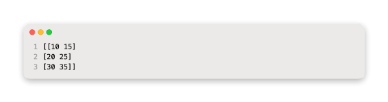
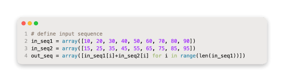
An example of this would be the addition of two parallel input time series.

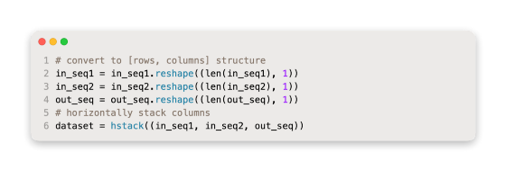
By reshaping these three arrays of data, we can make a single dataset containing time steps along with time series in columns. Parallel time series are stored in a CSV file in this manner.

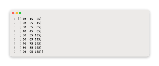
Below is an example in its entirety.

Taking the example as a whole, one row is printed per timestep, and one column is printed for each parallel input and output.

We must structure these data as samples with inputs and outputs, just as we did with the univariate time series.
In order to maintain the order of observations across the two input sequences, we need to divide the data into samples.
Here is a sample if we choose three input time steps:
The input is:

Output:
In this example, the model incorporates the first three time steps of each parallel series as input, and it associates the value of the third time step with the value of the output series.
As some values will be discarded from the output time series that were not included in the input time series at previous time steps of the training process, we will need to transform the time series into input/output samples. Depending on how many input time steps are chosen, the amount of training data will be used.
In this example, we will define a function called split_sequences() which will return input/output samples from a dataset with columns for parallel series and rows for time steps.

For each input time series, we can use three time steps to test this function.
Below is the complete example.

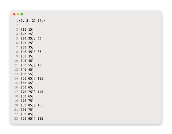
The first step when running the example is to print the shape of the X and Y components.
There is a three-dimensional structure to the X component.
In this case, there are seven samples in the first dimension. In this case, the function specifies a value of 3 for the number of time steps per sample. In this case, two parallel time series are listed in the last dimension, which specifies the number of variables.
There are then three time steps for each of the two input series for each sample, as well as the corresponding outputs for each sample.
We must flatten the input samples before we can fit an MLP to them.
A vector-shaped input portion is required for MLPs. In a multivariate input, each time step will be represented by a different vector.
The temporal structure of each input sample can be flattened as follows:
Becomes:

Using the number of features or the number of time steps, we can calculate the length of each input vector. Using this vector size, the input can be reshaped.

By using the vector length for the input dimension argument, we can now define an MLP model for the multivariate input.

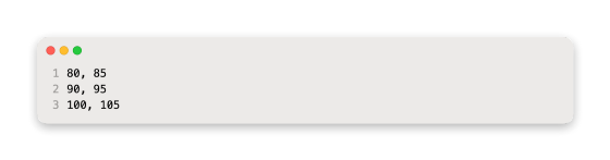
In order to make a prediction, the model expects two input time series to be separated by three time steps.
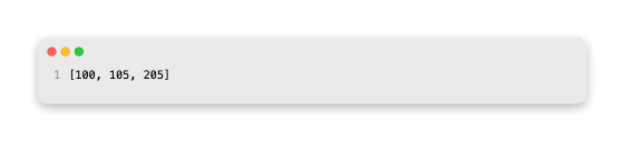
If we prove the following input values, we can predict the next output value:

Using 3 time steps and 2 variables, the shape of the 1 sample would be [1, 3, 2]. Using [1,6] as a vector of 6 elements, we must again reshape this to 1 sample.
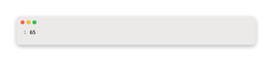
100 + 105 or 205 would be the next value in the sequence.

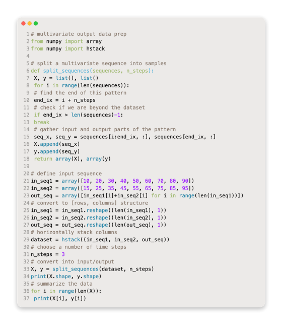
Below is an example in its entirety.
| # multivariate mlp example | |
| from numpy import array | |
| from numpy import hstack | |
| from keras.models import Sequential | |
| from keras.layers import Dense | |
| # split a multivariate sequence into samples | |
| def split_sequences(sequences, n_steps): | |
| X, y = list(), list() | |
| for i in range(len(sequences)): | |
| # find the end of this pattern | |
| end_ix = i + n_steps | |
| # check if we are beyond the dataset | |
| if end_ix > len(sequences): | |
| break | |
| # gather input and output parts of the pattern | |
| seq_x, seq_y = sequences[i:end_ix, :-1], sequences[end_ix-1, -1] | |
| X.append(seq_x) | |
| y.append(seq_y) | |
| return array(X), array(y) | |
| # define input sequence | |
| in_seq1 = array([10, 20, 30, 40, 50, 60, 70, 80, 90]) | |
| in_seq2 = array([15, 25, 35, 45, 55, 65, 75, 85, 95]) | |
| out_seq = array([in_seq1[i]+in_seq2[i] for i in range(len(in_seq1))]) | |
| # convert to [rows, columns] structure | |
| in_seq1 = in_seq1.reshape((len(in_seq1), 1)) | |
| in_seq2 = in_seq2.reshape((len(in_seq2), 1)) | |
| out_seq = out_seq.reshape((len(out_seq), 1)) | |
| # horizontally stack columns | |
| dataset = hstack((in_seq1, in_seq2, out_seq)) | |
| # choose a number of time steps | |
| n_steps = 3 | |
| # convert into input/output | |
| X, y = split_sequences(dataset, n_steps) | |
| # flatten input | |
| n_input = X.shape[1] * X.shape[2] | |
| X = X.reshape((X.shape[0], n_input)) | |
| # define model | |
| model = Sequential() | |
| model.add(Dense(100, activation='relu', input_dim=n_input)) | |
| model.add(Dense(1)) | |
| model.compile(optimizer='adam', loss='mse') | |
| # fit model | |
| model.fit(X, y, epochs=2000, verbose=0) | |
| # demonstrate prediction | |
| x_input = array([[80, 85], [90, 95], [100, 105]]) | |
| x_input = x_input.reshape((1, n_input)) | |
| yhat = model.predict(x_input, verbose=0) | |
| print(yhat) |
Preparing the data, fitting the model, and making a prediction is part of running the example.

The problem can also be modeled in a more elaborate way.
A separate MLP can handle each input series, and then the outputs of each submodel can be combined before the output sequence is predicted.
A multi-headed input MLP model can be described as such. Based on the specifics of the problem being modeled, it may offer more flexibility or better performance.
Keras’ functional API allows the definition of this type of model.
Firstly, let’s create an MLP that has an input layer with a feature set of n_steps vectors.

As with the first input submodel, the second can be defined similarly.

In order to predict the output sequence, we need to merge the output from each input submodel into a long vector.
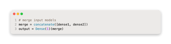
Afterwards, we can connect the inputs and outputs.

In the diagram below, the inputs and outputs of the layers are shown, along with the model’s schematic.

Forecasting multiple time series with a multiheaded MLP plot
Consequently, this model requires input as a list of two elements, each containing data for one of the submodels.
It is possible to achieve this by dividing the 3D input data into two separate 2D arrays with the shapes [7, 3, 2].

It is possible to provide these data in order to fit the model.

It is necessary to prepare two separate two-dimensional arrays for a single one-step prediction.

This is illustrated in the following example.

As part of running the example, you’ll need to prepare the data, fit the model, and make a prediction.

Parallel series of events
Known as an alternate time series problem, it involves predicting multiple parallel time series with varying values.
For example, based on the data in the previous section:
Each of the three time series has a next time step value that we would like to predict.
It might be called multivariate forecasting if it is based on multiple variables.
Splitting input and output samples is necessary for training a model.
The following samples would be included in this dataset:
The input is:

Output:

Split_sequences() is used to split multiple parallel time series into input/output shapes with rows representing time steps and columns representing series.
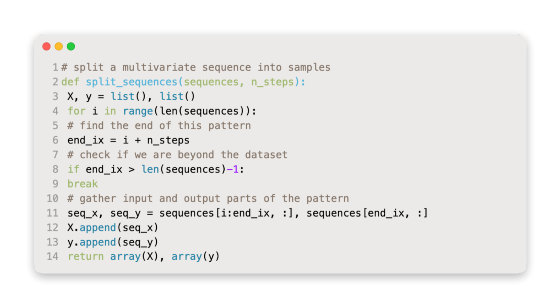
This can be demonstrated with the contrived problem; the full example is given below.
Following the run of the example, the X and Y components are printed in their respective shapes.
The X time series has three dimensions: six sample points, three time steps, and three parallel features.
Y has a two-dimensional shape when there are 6 samples and 3 variables to predict per sample.
The inputs and outputs of each sample are then printed.

A MLP model can be fitted to the data now that we have it.
Just as with multivariate input, we treat lag observations as features, so we flatten the input data samples into two dimensions [samples, features].

An element of a vector will be assigned to each of the three time series.

For the input layer, the flattened vector length can be used, while the vector length for the prediction layer can be the number of time series.

Providing three time steps for each of the three parallel series allows us to predict the next value.

The prediction must be based on one sample, three time steps, and three features. To match the expectations of the model, we can flatten this to [1, 6].
Here is an example of the vector output:

Here is an example of how an MLP can forecast output multivariate time series.

In running the example, the data is prepared, the model is fitted, and predictions are made.
Sequences can be predicted using a model.
Models with multivariate MLPs
There are multivariate time series when there are more than one observation per time step.
Two main models may be needed when dealing with time series data with multivariate components:
Multiple Input Series.
Multiple Parallel Series.
Let’s take a look at each one in turn.
Multiple Input Series
It is possible for a problem to have multiple parallel input time series and for the output time series to be dependent upon the input time series.
Time series inputs are parallel because each point is observed.
Taking two parallel time series inputs and adding their outputs as an example.
Rows represent time steps and columns represent time series, which can be combined into one dataset. CSV files store parallel time series in this manner.
A complete example can be found below.

In this example, one column is printed for each parallel input and output, and one row is printed for each timestep.

We must structure these data as samples with inputs and outputs, just as we did with the univariate time series.
In order to maintain the order of observations across the two input sequences, we need to divide the data into samples.
The first sample would look as follows if we chose three input time steps:
Input:

Output:

Specifically, input is provided for the first three time steps of each parallel series, and output is associated with the third time step value of 65 in this example.
Because some values in the output time series must be discarded since they were not in the input time series at the previously trained model’s time steps, we will need to turn the time series into input/output samples. According to how many input time steps are chosen, the training data will be used to a greater or lesser extent.
In this example, we will define a function called split_sequences() which will return input/output samples from a dataset with columns for parallel series and rows for time steps.

For each input time series, we can use three time steps to test this function.
Below is the complete example.

The example prints out the shape of the components X and Y first.
There is a three-dimensional structure to the X component.
In this case, there are seven samples in the first dimension. In this case, the function specifies a value of 3 for the number of time steps per sample. In this case, two parallel time series are listed in the last dimension, which specifies the number of variables.
There are then three time steps for each of the two input series for each sample, as well as the corresponding outputs for each sample.

We must flatten the input samples before we can fit an MLP to them.
A vector-shaped input portion is required for MLPs. Each time step will have its own vector when we receive a multivariate input.
Each input sample’s temporal structure can be flattened so that:

Becomes:

A vector’s length is calculated by multiplying the time steps by the number of features or series. The input can then be reshaped using this vector size.

By using the vector length for the input dimension argument, we can now define an MLP model for the multivariate input.

In order to make a prediction, the model expects two input time series to be separated by three time steps.
If we prove the following input values, we can predict the next output value:
One sample containing three time steps and two variables would look like [1, 3, 2]. To make this a single sample with 6 elements, we must reshape it to [1, 6].
Assuming the sequence continues, 100 + 105 or 205 should be the next value.

Below is an example in its entirety.

Preparing the data, fitting the model, and making a prediction is part of running the example.

The problem can also be modeled in a more elaborate way.
A separate MLP can handle each input series, and then the outputs of each submodel can be combined before the output sequence is predicted.
A multi-headed input MLP model can be described as such. Based on the specifics of the problem being modeled, it may offer more flexibility or better performance.
Using Keras’ functional API, this type of model can be defined.
First input models can be defined as MLPs with an input layer containing vectors with n_step features.

The second input submodel can be defined similarly.

In order to predict the output sequence, we need to merge the output from each input submodel into a long vector.

Afterwards, we can connect the inputs and outputs.

In the diagram below, the inputs and outputs of the layers are shown, along with the model’s schematic.

Forecasting multivariate time series with multiheaded MLPs