Forecasting Timeseries Using Machine Learning & Deep Learning

A forecasting LSTM model and a simple Ridge regression model are used in this post to predict stock prices.

Onepagecode

Mar 12, 2023

∙ Paid

1. Introduction

1.1. Models for time-series analysis and forecasting

Observations without a time dimension are used in most machine learning models.

The time-series forecasting model predicts future values by analyzing past values. Temperature, stock prices, and house prices are examples of non-stationary data, which show changes in their statistical properties over time. By analyzing data taken sequentially over time, these models analyze a signal.

Disclaimer (before moving on): Time series analysis algorithms can be used to predict stock prices, but they cannot be used to make real-time predictions. There is no intent in this article to "direct" people in any way to buy stocks.

2. We will use the following models:

Deep learning (LSTM)

The LSTM architecture is an artificial recurrent neural network (RNN) algorithm used in deep learning [1]. A LSTM has feedback connections as opposed to a feedforward neural network. Additionally, it can process whole sequences of data (such as speech or video inputs) in addition to single data points (e.g., images). It is possible to store information over a long period of time with LSTM models. Time-series or sequential data are extremely useful when we have this characteristic.

Regression with ridges (ML)

In linear regression, ridge regression is used to address the multicollinearity problem [2].

It reduces coefficients of predictors towards zero (also known as the L2 penalty) when ridge regression is applied to a linear regression model.

3. Data on the history of stock prices

We can access the data for free thanks to Yahoo Finance. Use the following link to get the stock price history of Apple: https://finance.yahoo.com/quote/AAPL/history?period1=1325376000&period2=1672531200&interval=1d&filter=history&frequency=1d&includeAdjustedClose=true

We will select a date range between 01/01/2012 and 01/01/2023. For your convenience, the data can also be downloaded.

To download the .csv file, click on the Download button and save it to your computer's hard drive.

Any stock you wish to trade, such as SPY, can be done the same way.

4. Python working example

The following modules are required: Keras, Tensorflow, Pandas, Scikit-Learn, Numpy, and Plotly

As an example, we will build a multilayer LSTM recurrent neural network to predict Apple's stock price.

The first thing we need to do is load the modules we need

import pandas as pd
import plotly.express as px
from scipy import stats
import numpy as np
import matplotlib.pyplot as plt
from sklearn.model_selection import train_test_split
from tensorflow import keras
from sklearn.preprocessing import MinMaxScaler
from sklearn.linear_model import Ridge
from sklearn.metrics import r2_score

# set plotly parameters
import plotly.io as pio
pio.renderers.default='notebook'

Now let’s read the data and store them in a pandas dataframe

# Read stock prices data
AAPL = pd.read_csv("AAPL.csv")
SP500 = pd.read_csv("SPY.csv")

# Select only the Date and Adj Close price
AAPL = AAPL[["Date", "Adj Close"]]
SP500 = SP500[["Date", "Adj Close"]]

# rename the columns
AAPL.rename(columns={"Adj Close": "AAPL"}, inplace = True)
SP500.rename(columns={"Adj Close": "SP500"}, inplace = True)

# concat all the data into one dataframe
stocks_df = pd.concat([AAPL, SP500.drop(columns=["Date"])], axis = 1)

# sort by date & visualize the df
stocks_df = stocks_df.sort_values(by = ['Date'])
stocks_df

       Date       AAPL       SP500
0  2012-01-03  12.500192  103.596214
1  2012-01-04  12.567369  103.758713
2  2012-01-05  12.706893  104.034943
3  2012-01-06  12.839727  103.766838
4  2012-01-09  12.819362  104.018715
...  ...  ...  ...
2763  2022-12-23  131.658981  382.910004
2764  2022-12-27  129.831772  381.399994
2765  2022-12-28  125.847855  376.660004
2766  2022-12-29  129.412415  383.440002
2767  2022-12-30  129.731918  382.429993

For normalization and plotting, let's create some custom functions

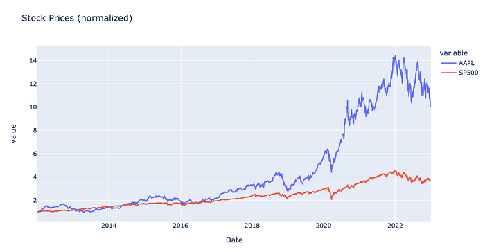
Using the initial price of the stock on January 1, 2012, we will normalize each stock.

# Plot interactive plots using Plotly
def plotl(df, title):
    fig = px.line(df, x='Date', y=df.columns[1:], title=title) # close price in y axis
    fig.show()

# normalize the prices and plot chart for AAPL
normalized_stocks_df = stocks_df.copy()
normalized_stocks_df.iloc[:, 1:] = normalized_stocks_df.iloc[:, 1:].div(normalized_stocks_df.iloc[0, 1:], axis=1)

plotl(normalized_stocks_df), 'Stock Prices (normalized)')