


From Data to Decisions: Python’s Role in Financial Forecasting
From Data to Decisions: Python’s Role in Financial Forecasting
Mastering Stock Market Forecasts with Alpha Vantage and PyTorch

Embark on a technical expedition into the realm of financial forecasting with Python. This article provides a deep dive into setting up the Alpha Vantage library for accessing detailed stock market data, and explores the implementation of deep learning models using PyTorch.
From the initial installation of libraries like NumPy and matplotlib for data manipulation and visualization, to configuring and training sophisticated LSTM networks for predictive accuracy, this guide covers the complete pipeline. With practical code snippets and configurations for managing data splits, training processes, and model evaluations, you’re equipped to harness the predictive power of machine learning to analyze and forecast stock market trends effectively.
Install libraries, setup PyTorch, Alpha Vantage, print message
! pip install alpha_vantage -q

import numpy as np

import torch
import torch.nn as nn
import torch.nn.functional as F
import torch.optim as optim
from torch.utils.data import Dataset
from torch.utils.data import DataLoader

import matplotlib.pyplot as plt
from matplotlib.pyplot import figure

from alpha_vantage.timeseries import TimeSeries

print("All libraries loaded")
The code snippet above serves to guide you in setting up the Alpha Vantage library through pip, pulling in vital libraries like NumPy, PyTorch, and Matplotlib, and establishing a framework for handling financial time series data in deep learning models.
Delving deeper into the code:
1. The Alpha Vantage Python package is installed to facilitate seamless access to stock market data.
2. NumPy supports numerical computations, PyTorch aids in constructing deep learning models, and Matplotlib is employed for generating visualizations.
3. Essential deep learning components are arranged, encompassing neural network layers, optimizers, datasets, and data loaders.
4. By importing the TimeSeries class from the Alpha Vantage library, the code retrieves historical financial data effortlessly.
5. A confirmation message signaling the successful loading of all libraries concludes the execution.
This code snippet is an invaluable resource for individuals keen on delving into financial time series data processing and constructing predictive models employing deep learning methodologies. Leveraging Alpha Vantage broadens access to financial market data, whereas NumPy, PyTorch, and Matplotlib streamline data manipulation, model development, and data visualization, respectively.
API key, data, plots, model, training details
config = {
    "alpha_vantage": {
        "key": "YOUR_API_KEY", # Claim your free API key here: https://www.alphavantage.co/support/#api-key
        "symbol": "IBM",
        "outputsize": "full",
        "key_adjusted_close": "5. adjusted close",
    },
    "data": {
        "window_size": 20,
        "train_split_size": 0.80,
    },
    "plots": {
        "show_plots": True,
        "xticks_interval": 90,
        "color_actual": "#001f3f",
        "color_train": "#3D9970",
        "color_val": "#0074D9",
        "color_pred_train": "#3D9970",
        "color_pred_val": "#0074D9",
        "color_pred_test": "#FF4136",
    },
    "model": {
        "input_size": 1, # since we are only using 1 feature, close price
        "num_lstm_layers": 2,
        "lstm_size": 32,
        "dropout": 0.2,
    },
    "training": {
        "device": "cpu", # "cuda" or "cpu"
        "batch_size": 64,
        "num_epoch": 100,
        "learning_rate": 0.01,
        "scheduler_step_size": 40,
    }
}
Contained within this script is a Python dictionary serving as the repository for setting configurations pertinent to a project focusing on financial data analysis and forecasting. Let’s delve into the breakdown of each segment in this configuration dictionary:
1. alpha_vantage: This section houses settings associated with the Alpha Vantage API, encompassing details like the API key, stock symbol, data output size, and the access key for adjusted close prices.
2. data: Here, you’ll find specifications pertaining to the dataset, including the window size utilized for feature engineering and the proportion for segmenting the dataset into training and validation subsets.
3. plots: This segment configures settings for showcasing plots, ranging from toggling plot visibility to setting x-axis tick intervals and assigning colors for actual data, training data, validation data, and predicted data in the plots.
4. model: This part lays out the parameters for the LSTM neural network model, outlining the input size, quantity of LSTM layers, LSTM unit size, and dropout rate aimed at curbing overfitting.
5. training: Steering various elements of the training procedure, this section dictates the device to employ (‘cpu’ or ‘cuda’ for GPU), batch size, epoch count, learning rate, and the increment size for the learning rate scheduler.
Such a configuration dictionary proves pivotal in upholding uniformity across assorted sections of the codebase while streamlining the process of adjusting configurations sans direct alterations to the source code. With a setup like this in place, experimenting with diverse parameters, datasets, and models turns into a more straightforward endeavor, minus the need for direct tweaks to the code.
Let’s delve into the data preparation phase of our project, where we will gather financial market data from Alpha Vantage.
This code downloads and plots daily stock data
def download_data(config, plot=False):

    ts = TimeSeries(key=config["alpha_vantage"]["key"])
    data, meta_data = ts.get_daily_adjusted(config["alpha_vantage"]["symbol"], outputsize=config["alpha_vantage"]["outputsize"])

    data_date = [date for date in data.keys()]
    data_date.reverse()

    data_close_price = [float(data[date][config["alpha_vantage"]["key_adjusted_close"]]) for date in data.keys()]
    data_close_price.reverse()
    data_close_price = np.array(data_close_price)

    num_data_points = len(data_date)
    display_date_range = "from " + data_date[0] + " to " + data_date[num_data_points-1]
    print("Number data points:", num_data_points, display_date_range)

    if plot:
        fig = figure(figsize=(25, 5), dpi=80)
        fig.patch.set_facecolor((1.0, 1.0, 1.0))
        plt.plot(data_date, data_close_price, color=config["plots"]["color_actual"])
        xticks = [data_date[i] if ((i%config["plots"]["xticks_interval"]==0 and (num_data_points-i) > config["plots"]["xticks_interval"]) or i==num_data_points-1) else None for i in range(num_data_points)] # make x ticks nice
        x = np.arange(0,len(xticks))
        plt.xticks(x, xticks, rotation='vertical')
        plt.title("Daily close price for " + config["alpha_vantage"]["symbol"] + ", " + display_date_range)
        plt.grid(b=None, which='major', axis='y', linestyle='--')
        plt.show()

    return data_date, data_close_price, num_data_points, display_date_range

data_date, data_close_price, num_data_points, display_date_range = download_data(config, plot=config["plots"]["show_plots"])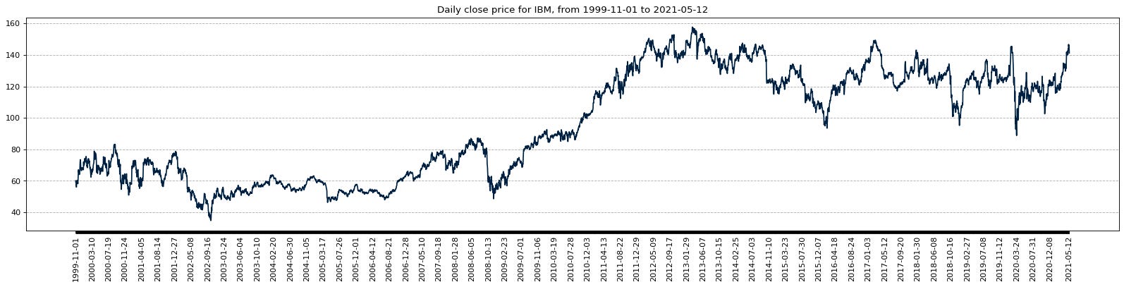
The code presented here establishes a function named download_data, responsible for fetching daily stock market data of a specified symbol via the Alpha Vantage API. By leveraging the predefined configuration settings, the function securely accesses the API, retrieves the data, and, if desired, crafts a visual representation.
To break it down:
1. It first imports essential libraries like TimeSeries to interact with the Alpha Vantage API and various plotting tools.
2. The function then reaches out to the Alpha Vantage API to procure daily adjusted data for a designated stock symbol, capturing both the data itself and accompanying metadata.
3. Subsequently, it handles the data by isolating dates and closing prices, reordering them to suit plotting requirements, and computes the data point count and date span.
4. If prompted with the plot flag as True, a graphical representation is formulated, exhibiting the daily closing prices alongside tailored x-axis markings and gridlines.
5. Finally, the function furnishes the extracted data encompassing dates, closing prices, data point quantity, and the range of dates shown.
This functionality is key for obtaining and illustrating daily stock market insights based on user-specified settings, thereby facilitating trend analysis and decision-making. By encapsulating the data retrieval and processing stages, this function enhances code structure, flexibility, and readability, advancing overall code quality.
A crucial step before analyzing financial data is data preparation, which involves normalizing raw data.
Class to normalize and inverse data
class Normalizer():
    def __init__(self):
        self.mu = None
        self.sd = None

    def fit_transform(self, x):
        self.mu = np.mean(x, axis=(0), keepdims=True)
        self.sd = np.std(x, axis=(0), keepdims=True)
        normalized_x = (x - self.mu)/self.sd
        return normalized_x

    def inverse_transform(self, x):
        return (x*self.sd) + self.mu

scaler = Normalizer()
normalized_data_close_price = scaler.fit_transform(data_close_price)
In this code, there is a class called Normalizer, designed for data normalization and inverse transformation. The fit_transform function computes the mean (mu) and standard deviation (sd) of the given data across a specific axis (axis 0) and then proceeds to normalize the data based on these computed values, delivering the normalized data as output.
For the inverse transformation, the inverse_transform method accepts normalized data and utilizes the previously determined mean and standard deviation to revert the normalization process, restoring the data to its original form.
Data normalization, a widely adopted data preparation procedure in both machine learning and data analysis, serves to adjust numerical data to a standard range. This step holds significance as numerous machine learning algorithms exhibit enhanced performance or quicker convergence when input features share a similar scale. The Normalizer class serves as a beneficial and reusable solution for normalizing and inversely transforming data efficiently for modeling tasks.
Let’s dive into data preparation by creating training and validation datasets.
Prepare and split data for training
def prepare_data_x(x, window_size):
    n_row = x.shape[0] - window_size + 1
    output = np.lib.stride_tricks.as_strided(x, shape=(n_row,window_size), strides=(x.strides[0],x.strides[0]))
    return output[:-1], output[-1]

def prepare_data_y(x, window_size):

    output = x[window_size:]
    return output

def prepare_data(normalized_data_close_price, config, plot=False):
    data_x, data_x_unseen = prepare_data_x(normalized_data_close_price, window_size=config["data"]["window_size"])
    data_y = prepare_data_y(normalized_data_close_price, window_size=config["data"]["window_size"])


    split_index = int(data_y.shape[0]*config["data"]["train_split_size"])
    data_x_train = data_x[:split_index]
    data_x_val = data_x[split_index:]
    data_y_train = data_y[:split_index]
    data_y_val = data_y[split_index:]

    if plot:

        to_plot_data_y_train = np.zeros(num_data_points)
        to_plot_data_y_val = np.zeros(num_data_points)

        to_plot_data_y_train[config["data"]["window_size"]:split_index+config["data"]["window_size"]] = scaler.inverse_transform(data_y_train)
        to_plot_data_y_val[split_index+config["data"]["window_size"]:] = scaler.inverse_transform(data_y_val)

        to_plot_data_y_train = np.where(to_plot_data_y_train == 0, None, to_plot_data_y_train)
        to_plot_data_y_val = np.where(to_plot_data_y_val == 0, None, to_plot_data_y_val)


        fig = figure(figsize=(25, 5), dpi=80)
        fig.patch.set_facecolor((1.0, 1.0, 1.0))
        plt.plot(data_date, to_plot_data_y_train, label="Prices (train)", color=config["plots"]["color_train"])
        plt.plot(data_date, to_plot_data_y_val, label="Prices (validation)", color=config["plots"]["color_val"])
        xticks = [data_date[i] if ((i%config["plots"]["xticks_interval"]==0 and (num_data_points-i) > config["plots"]["xticks_interval"]) or i==num_data_points-1) else None for i in range(num_data_points)] # make x ticks nice
        x = np.arange(0,len(xticks))
        plt.xticks(x, xticks, rotation='vertical')
        plt.title("Daily close prices for " + config["alpha_vantage"]["symbol"] + " - showing training and validation data")
        plt.grid(b=None, which='major', axis='y', linestyle='--')
        plt.legend()
        plt.show()

    return split_index, data_x_train, data_y_train, data_x_val, data_y_val, data_x_unseen

split_index, data_x_train, data_y_train, data_x_val, data_y_val, data_x_unseen = prepare_data(normalized_data_close_price, config, plot=config["plots"]["show_plots"])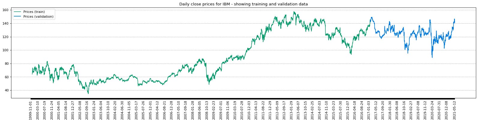
The provided code snippet introduces functions geared towards data preparation for a machine learning model. This includes the prepare_data_x function, which generates input data (data_x) through a sliding window technique applied to normalized close price data. By segmenting the data into subsets determined by a specified window size, it lays the foundation for subsequent analysis. On the other hand, the prepare_data_y function creates output data (data_y) by shifting the input data by the window size.
Furthermore, the prepare_data function amalgamates the aforementioned data preparation operations. It divides the input and output data into training and validation sets using a designated split size. In case the plot parameter is activated, a visual representation of the training and validation data is generated.
This code plays a pivotal role in the machine learning workflow as it orchestrates data structuring conducive to model training and performance assessment. By guaranteeing the correct alignment of input and output data for the machine learning algorithm to discern patterns and offer projections, it sets the stage for informed decision-making. Additionally, the visualization component enriches the comprehension of data distribution and trends, which are instrumental in scrutinizing and interpreting model performance.
Convert time series data for LSTM
class TimeSeriesDataset(Dataset):
    def __init__(self, x, y):
        x = np.expand_dims(x, 2) # in our case, we have only 1 feature, so we need to convert `x` into [batch, sequence, features] for LSTM
        self.x = x.astype(np.float32)
        self.y = y.astype(np.float32)

    def __len__(self):
        return len(self.x)

    def __getitem__(self, idx):
        return (self.x[idx], self.y[idx])

dataset_train = TimeSeriesDataset(data_x_train, data_y_train)
dataset_val = TimeSeriesDataset(data_x_val, data_y_val)

print("Train data shape", dataset_train.x.shape, dataset_train.y.shape)
print("Validation data shape", dataset_val.x.shape, dataset_val.y.shape)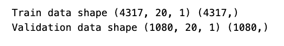
The code provided here presents a custom dataset class named TimeSeriesDataset, which is a subclass of the Dataset class. Its main objective is to format time series data to be compatible with training neural networks, particularly those utilizing LSTM (Long Short-Term Memory) architecture.