

Hands-On Machine Learning With Scikit-Learn
As you are reading this article, chances are that you have heard of Deep Learning, a technique that has become increasingly popular in recent years.

As a subset of the wider field of Machine Learning, Deep Learning is a subset of what Machine Learning is all about. In different fields, such as finance, education, medicine, and basic science, there are many traditional algorithms that are in use today. While Deep Learning is considered to be a silver bullet, there are still many situations and tasks in which traditional Machine Learning is required.
Is traditional machine learning still necessary?
The question may arise in some people's minds as to why we need traditional machine learning when Deep Learning is so great. Deep Learning has its limitations, and that is a simple answer to the question.
This is due to the fact that Deep Learning is a black box, which means that we have no idea why it gives such outputs based on what we input. Traditionally, there are some forms of Machine Learning that are interpretable, such as linear regression and decision trees. There are some areas in which interpretability is important.
The process of deep learning generally requires a large amount of data to be collected. As a result, in the real world, there are times when there is not enough data for some tasks to be completed. Small data sets can be easily handled by traditional Machine Learning techniques.
The benefits of deep learning are not significant for some problems, as they are relatively simple. It is possible to achieve the same results with less effort by using simple solutions.
Traditional Machine Learning is the only way to solve some problems.
Exactly what we need is Scikit-learn.
In addition to being a free machine learning library, Scikit-Learn is also known as sklearn. In addition, to support vector machines, random forests, gradient boosting, k-means, and DBSCAN, it includes various algorithms for classification, regression, and clustering. In addition to the features above, sklearn also provides feature extraction, feature selection, model evaluation, model selection, parameter tuning, and dimension reduction, among others. A complete Machine Learning project would not be complete without these components.
As a result of the limited scope of this course, we will not be covering the theory or mathematics behind any of these algorithms. Each lesson will introduce some background knowledge, but the main goal is to help you use this library in the real world in order to solve real-world problems.
What makes Sklearn so special?
Learning and using it is easy.
Machine Learning is covered in all aspects, including Deep Learning.
There are many things you can do with it, and it’s very powerful.
An active community, detailed documentation, and open-source software.
Among Machine Learning toolkits, it is the most widely used.
What you will learn from this Article?
Some models for supervised learning, such as
Logistic Regression,SVM, andNaive BayesTree-based models such as
decision treeandGBDTClustering methods such as
kmeansFeature engineering such as
feature selection,feature extraction, anddimension reductionData preprocessing
Model evaluation
Hyperparameter searching
Simple neural network
Load Built In Datasets
We will be covering the topic of datasets in this lesson. In order to complete a Machine Learning project, a dataset is an essential part of the process since it is the starting point of the project.
There are a multitude of datasets that are included in the scikit-learn library, some of which are well known and are widely used. As an example, the datasets used by the program include those for classification and regression, for example, the iris and mnist datasets. The scikit-learn library provides additional functions in addition to the predefined datasets that allow the user to generate data that follows a specific distribution in addition to these predefined datasets.
In the meantime, scikit-learn has predefined some functions which can be used for downloading real-world datasets from the internet, such as the 20 newsgroups dataset, the LFW dataset, or KDDcup99 dataset.
This module datasets contains all of the datasets that are available. This module should be imported at the beginning of your Python file in the following way.
import sklearn.datasets as datasetsLoad built-in dataset
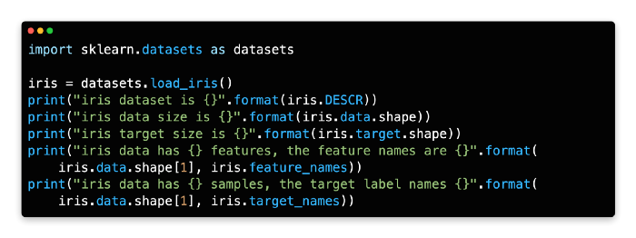
Scikit-learn provides some built-in datasets, including the iris, as mentioned above. The only function you need is load_iris, as shown below.
import sklearn.datasets as datasets
iris = datasets.load_iris()
Datasets contain all the necessary data and metadata in a dictionary-like structure. A 2D array of n_samples * n_features is used to store the data in the field data. In the field target, the label is stored.
You can get the size and feature name of the data using the code below.
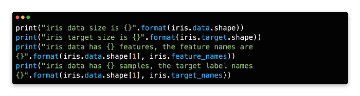
By using the built-in function load_iris(), the built-in Iris dataset is loaded into memory.
The following table shows some important attributes of this dataset from lines 4 to line 9. Sklearn’s built-in datasets have the same characteristics that can be found in most of its datasets.
Generate classification dataset
There are a few functions provided by scikit-learn to help you create artificial datasets, as I mentioned above. From the code below, it can be seen that make_classification generates a random n-class classification dataset based on the code you provide.
There is a default number for the number of classes in the application, which is 2. It can be changed from the parameter n_classes if you wish.
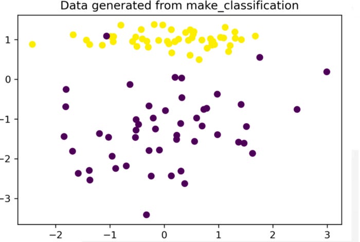
Here is an example of data that has two class labels with two features in the data below. During the course of the function, there are two variables returned. The first variable, X, is a 2D array containing an array of n_samples and n_features, which is a 2D array of samples, just as the field in the iris data is an array of samples. Secondly, there is a vector called y, which represents the target.
X,y = datasets.make_classification(n_features=2,
                                   n_redundant=0, n_informative=1,n_clusters_per_class=1)
print("The data X shape is {}".format(X.shape))
print("The data y shape is {}".format(y.shape))
In order to draw a 2D chart, we simply have to draw two classes and assign different colors to each of them since this is a two-class classification data with two features.
If you are interested in seeing the difference between two outputs, you can try changing the parameters in the code widget below and then re-run the code to see what happens.
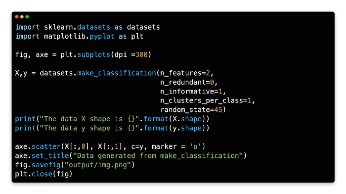
A classification dataset can be created by calling make_classification on line 6 of the code. There are a number of parameters that need to be considered here:
n_features: The total number of features.
n_informative: The number of informative features. The number of features in a website that provides useful information is, in other words, the number of features.
n_redundant: The number of redundant features. Typically, these features are generated by combining a set of informative features in a linear fashion.
n_clusters_per_class: The number of clusters per class.
You can check the full list from this link.
In line 11, it prints the shape of the dataset and in line 12, it prints the shape of the dataset.
From line 14 to line 17, this dataset has been plotted on a graph. In this example, we use the
scattertype. You can check the image above.
c=y means the point’s color is yellow, so it has a parameter c for color. You can pass c=r to create a red marker.
Marker style is specified by the parameter marker. A circle would be used as a marker in this example.
Regression dataset generation
We generated classification data in the last section, which is similar to generating regression data. Making a regression dataset is as simple as using make_regression. The data in our demo is linearly related to the target and we create one feature per dataset.
X, y = datasets.make_regression(n_features=1, n_informative=1)
print("The regression data X shape is {}".format(X.shape))
print("The regression data y shape is {}".format(y.shape))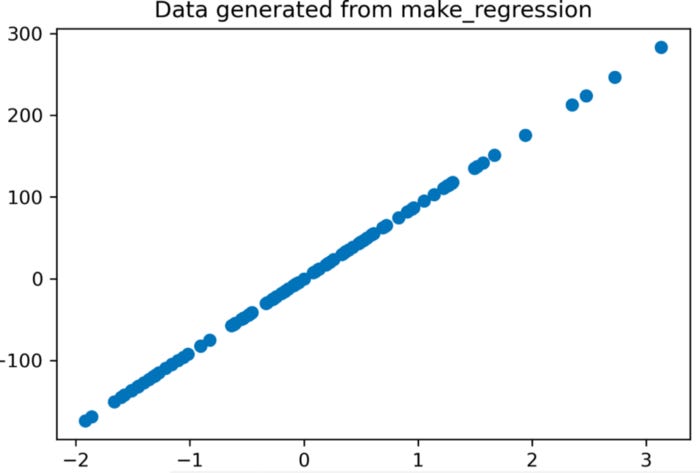
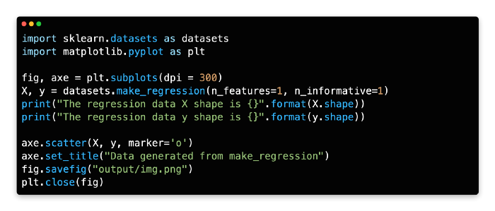
By using make_regression, a regression dataset can be created. The last section of this article explains the parameters this function supports.
It prints the shape of this dataset from line 6 to line 7.
Line 9 to line 12 are plotted in this dataset. The scatter type is used in this example.
Data Preprocessing
As we all know, data is not perfect when it comes to the real world. Data preprocessing is an important part of the analysis process, and it involves many steps, such as cleaning, scaling, normalizing, and so on. Throughout the entire Machine Learning process, the preprocessing of data may be one of the most important steps. There’s a common saying that goes “Garbage in, garbage out” and I’m sure you’ve heard it before. A good model will not be able to produce an ideal result if there is a poor quality of data, no matter how sophisticated it may be. In most cases, engineers spend 70 percent of their time processing data, which is typical for most of their jobs.
To change the raw feature vectors into a more appropriate representation suitable for downstream estimators, the preprocessing package provides a number of common utility functions and transformer classes.
It is important to note that there are many types of preprocessing. It will be the purpose of this lesson to cover some of the most common methods that are used in the field. The Jupyter file that is attached at the end of this lesson will allow you to learn more about what we have discussed so far.
Scale numerical feature
There is a good chance that the features in your dataset will vary in terms of their range most of the time. There is, however, a wide range of Machine Learning algorithms that determine the distance between two data points by using Euclidean distances as the metrics. The problem here is that there is nothing that can be done about it. The first thing we need to ensure is that the features are within the same range of values in this case. This problem can be solved by scaling your data in order to solve it. It is possible to accomplish this in a number of ways.
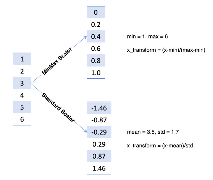
MinMax
As a result, it shrinks the range from zero to one.
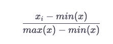
According to the code below, a function MinMaxScaler would take a value and scale it from zero to one, column-by-column.
import sklearn.preprocessing as preprocessing

minmax = preprocessing.MinMaxScaler()
# X is a matrix with float type
minmax.fit(X)
X_minmax = minmax.transform(X)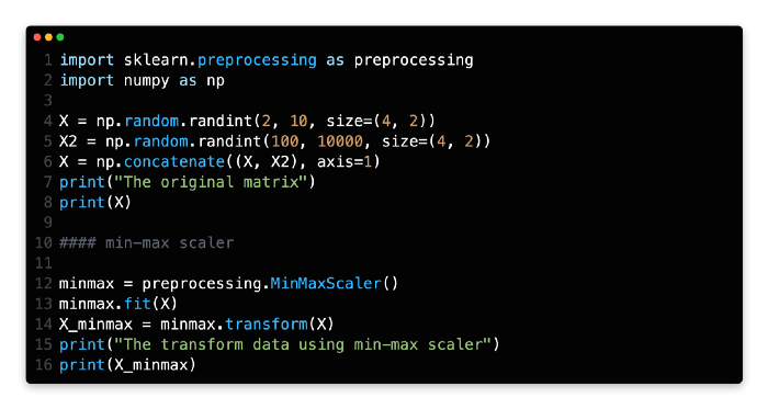
First of all, we are going to use Numpy randint to create a matrix with a width of four rows and two columns, whose number ranges from two to ten, and a size of four rows and two columns. We then create another matrix, the size of which is the same as the first one, and whose numbers range from 100 to 1,000. A concatenation of these two metrics results in a single metric. Based on the output of line 8, one can see that the range of numbers for each column varies greatly from one column to the next.
As you can see in line 12, the MinMaxScaler class is used to create a min-max scaler.
At line 14, the original matrix is fitted and transformed in order to get the new matrix.
Take a look at the new data at line 16 to see if it matches the old one.
Standard
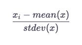
It is assumed that the distribution of your feature follows a normal distribution when you use this scaler. After calculating the mean and standard deviation for the feature you wish to scale, the following scaling function is applied to that feature before it is scaled.
A function StandardScaler would scale the values, as shown in the code below.
std = preprocessing.StandardScaler()
# X is a matrix
std.fit(X)
X_std = std.transform(X)
Please see the Jupyter file at the end of this lesson for more information on scale types and examples. The next type of preprocessing is now available to us and we can move forward with it.
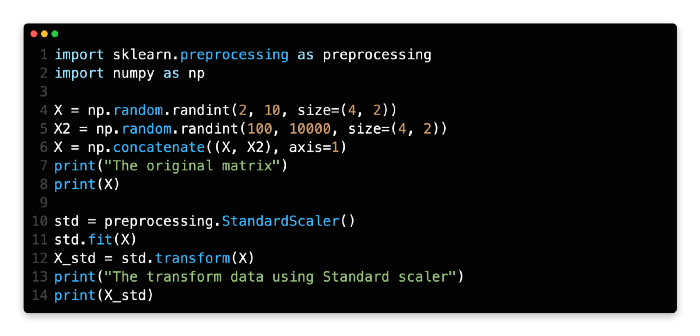
To begin with, we will use Numpy randint to create a matrix whose size will be four rows and two columns, and whose number will range between two and ten. We will then create a second matrix with the same size, but this one will have numbers ranging from 100 to 1,000. Line 6 of the matrix represents a concatenation of these two metrics to create a single metric.
As you can see in line 10, we are creating a Standard scaler by using the StandardScaler class.
In line 12, we are going to fit the original matrix and transform it into the new matrix.
The new data can be found at line 16 if you check the new data there.
Numerical feature mapping with non-linearity
We want to be able to map some numerical features in a nonlinear way, such as binarizing based on a threshold or bucketing based on points, for instance.
Binarizer
Binarizers set feature values to zero or one based on thresholds. Here, we set values larger than 0.7 to one because the threshold is 0.7.
binary = preprocessing.Binarizer(threshold=0.7)
X_binary = binary.transform(Xb)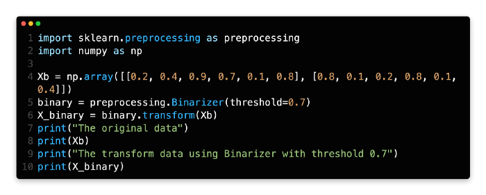
In line 4, a matrix with values ranging from zero to one is created.
There is a Binarizer object that is created at line 5 with a threshold value of 0.7. Once that Binarizer object has been created, the original data will then be transformed at line 6. There should be only zero/one values in the matrix at line 10, but if so, you could check the result at line 10.
Working with categorical features
Until now, all of the data we have been discussing has been of a numerical nature. Quite a few characteristics in real data can be categorical in nature. It is also important to note that all the data in Natural Language Processing is text and not numbers. There are a lot of methods that can be used to transform categorical data into numerical data in this section, so we will learn some of them.
Label encoder
There are times when we do not have a number on our label, but a string instead. This string is going to be converted to a number that starts from zero. As far as binary classification is concerned, there are two labels available: zero and one. The label will be zero if the classification is three classes, one if it is two, and three if it is three classes. As long as you have a value between zero and n_classes-1, LabelEncoder can be used to encode labels.

A category array is created in line 4.
The label encoder object is created in line 5. A fit and transform are then applied to the original array.
It is evident at line 11 that the Sun is encoded as 3, the Moon as 2, and so on.
The Jupyter widget below will let you see a few other preprocessing techniques in action once we have covered a few preprocessing techniques.
Feature Selection
It is the process of selecting a subset of relevant features (variables, predictors, etc.) that will be used in the construction of a machine learning model that uses feature selection. Machine Learning projects require this step, which is also referred to as feature engineering. The following reasons make this important:
For the purpose of reducing training time. Feature space and training time are positively correlated.
The curse of dimensionality must be avoided.
Streamline the model.
Overfitting should be reduced and generalization should be improved.
Enhance interpretability and reduce collinearity.
Datasets (tables) consist of columns that are features, but not all columns are useful or relevant. A little time should be spent on feature selection. In feature selection, the premise is that the data contains redundant or irrelevant features that can be removed without compromising the accuracy of the data.
Feature selection can be done in a number of ways. We will cover a number of functions available in Sklearn in the following section.
Low variance features should be removed
When a feature has zero variance, what does that mean? All instances of this feature share the same value since this feature has only one value. It doesn’t contain any information and doesn’t contribute to the prediction of the target. Similarly, features with low variance contain little information about the target, so they can be removed without hurting the model’s performance.
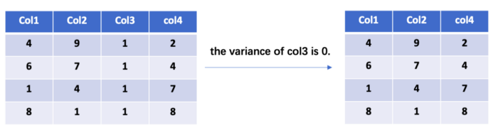
It is possible to remove low variance features using Sklearn’s VarianceThreshold. You can control the variance threshold with threshold.
import sklearn.feature_selection as fs

# X is you feature matrix
var = fs.VarianceThreshold(threshold=0.2)
var.fit(X)
X_trans = var.transform(X)
Here is a code example that you can try out. There is one value that is different between the first feature and the second feature, so it is removed from the first column, as you can see.
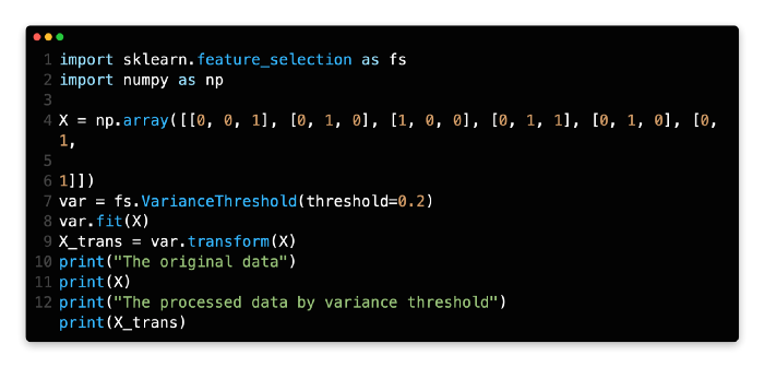
In line 3, we create a matrix that has a size of six rows and three columns.
In line 6, the VarianceThreshold object is created using the parameter threshold=0.2, which means that columns with a variance less than 0.2 will be removed from the dataset as a result of creating the variance threshold object.
The original matrix can be compared with the new matrix by going to line 12 and comparing the two.
Feature selection for K-best
There is a function provided by Sklearn called SelectKBest which can be used to select k best features based on some metric of your choice, and all you need to do is provide a score function to define the metric. Thanks to Sklearn, there are some predefined scoring functions that can be made use of. In this section, you will find some predefined functions that can be called to calculate scores.
In a classification task, the f_classif variable represents the F-value for the ANOVA between label and feature.
There are two types of mutual information: mutual_info_classif and mutual_info_discrete.
The chi-squared statistic is used to calculate the number of non-negative features in classification tasks.
For regression tasks, the f-value is calculated between the label and the feature.
In mutual_info_regression, a continuous target is provided with mutual information.
Using the false positive rate test, select features that are likely to result in false positives.
This method basically involves calculating a set of metrics between the target and each feature, sorting them, and then selecting the K best features as the result.
Here we are going to use the f_classif as the metric and K as the number of classes.
import sklearn.datasets as datasets
X, y = datasets.make_classification(n_samples=300, n_features=10, n_informative=4)
# choose the f_classif as the metric and K is 3
bk = fs.SelectKBest(fs.f_classif, 3)
bk.fit(X, y)
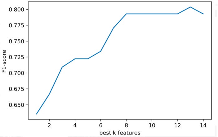
X_trans = bk.transform(X)It is important to investigate how reducing the number of features affects the model’s performance. Here is an example of comparing the performance of different logistic regressions based on different K best features.
From the image below, it can be seen that removing just a few features won’t have a large impact on the metric.
Here is the code you can try. When creating a new dataset, simply change the number of features or the number of K.
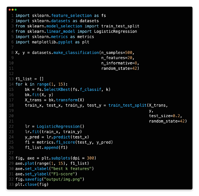
The first step is to create a classification dataset using make_classification on line 8.
There is a loop for k in range(1, 15) from line 14 to line 26. SelectKBest would receive a different value of K in each iteration of this loop. In order to examine the performance of the model, we want to see how the value of K affects it. Each time the loop is iterated (from line 22 to line 25), a logistic regression model is built, fit, and evaluated. A list, f1_list, contains the metrics. Our metric is the f1-score in this demo.
In the plot below, we plot the f1-scores for those Ks from line 28 to line 33.
Choose a feature from another model
In addition to any estimator which has a coef_ or feature_importances_ attribute after fitting, SelectFromModel can be used as a meta-transformer. However, we are only interested in the tree-based model. Several metrics are used to split the tree by a single feature. The importance of different features can be determined based on this metric. A tree model has this property, so we know how different features contribute to the model through the tree model.
In the next lecture, we will discuss the model (GBDT) mentioned here.
SelectFromModel is provided by Sklearn for selecting features. The first parameter in the code below is gb. This is a GBDT model that uses feature_importances_ to select features. Feature selection is easy with tree models.
import sklearn.feature_selection as fs

model = fs.SelectFromModel(gb, prefit=True)
# X is your feature matrix, X_trans is the new feature matrix.
X_trans = model.transform(X)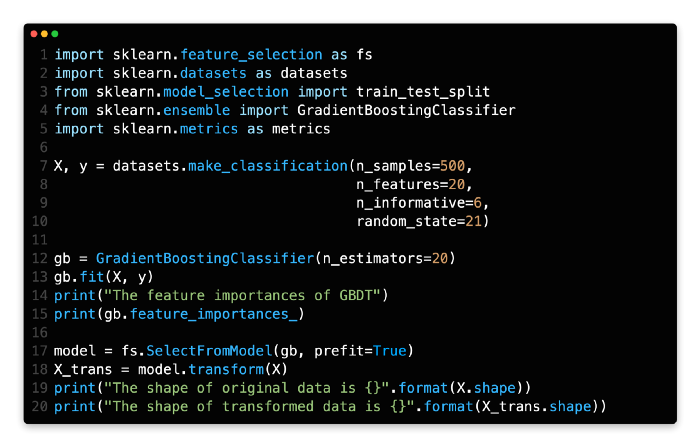
It is at line 7 that a dataset is created.
The GradientBoostingClassifier object is then converted into a GBDT object and the fit of the GBDT object is done at line 13.
Using the output of line 15, we can see the importance of different features based on their numbers. The higher the number, the more important the feature is.
It is shown in line 17 how to select a feature from another model by using the SelectFromModel method. It is just a matter of passing the GBDT object to the function. Having the prefit=True indicates that the model has already been fitted and is ready for use.
Using the widget, you can open the Jupyter file below, which contains additional content and interactive operations, that can be accessed by launching the widget.
Feature Extraction
The process of extracting features differs from the process of selecting features. Feature extraction refers to the process of extracting data from complex data, such as text or images, so that numerical features can be extracted from them. The processing of images and the processing of text are complex structured data types that cannot be directly processed by traditional Machine Learning algorithms. Feature extraction must be performed on such data to prepare it for downstream processing. In deep learning, end-to-end training is possible; for example, a neural network can process raw JPEG files without any manual intervention.
In this lesson, we will only focus on text, as the sklearn provides some functions to process image and text.
Machine Learning algorithms are often used to process text. It is not possible for models to process raw data (a sequence of tokens) directly. The raw data must be processed and some numerical feature vector extracted for the model. Text files are vectorized in general when they are converted into numerical feature vectors.
What is sparsity?
Natural language is characterized by sparsity. In the case of vectorization, its length is generally calculated according to the size of the vocabulary in the corpus. The length of the vector is determined by the size of the vocabulary, which in this case will be ten thousand. In the case of a relatively short text, there will be a limited number of tokens, and the rest will be zeroes, because the tokens are limited.
How does CountVectorizer work?
With CountVectorizer, you can tokenize and count occurrences in the same class. Many useful parameters are available. Let’s see what we can find.
Remove accents with strip_accents.
Lowercase: All characters are converted to lowercase.
The preprocessor is a callable function that preprocesses the text.
Default tokenizer can be overridden by this callable function.
The stop_words function removes very common words, such as the, a, and and. The built-in list of words can be used or you can pass a list of words.
A tuple containing ngram_range. Unigrams are the default (1, 1), so the default is (1, 1). In the case of (2, 2), only bigrams will be accepted. It means unigrams and bigrams if you pass (1, 2).
By default, the analyzer is set to word, which means the feature is based on words. Passing char indicates that the feature is based on characters.
The maximum value of max_df is between 0 and 1. Terms with a document frequency exceeding the threshold should be ignored when building the vocabulary.
The minimum and maximum values of min_df. Do not include terms in the vocabulary whose document frequency is strictly below the given threshold.
The max_featuresint parameter specifies whether to build a vocabulary that only takes into account the top max_features based on term frequency.
CountVectorizer can be used in a variety of ways. CountVectorizer objects are created by calling CountVectorizer(), the corpus is fitted, and then the corpus is transformed. Each sample would have a matrix showing the count of each word.
from sklearn.feature_extraction.text import CountVectorizer

counterVec = CountVectorizer()
# corpus is a list of string in this example, such as:
# corpus = [
#    "I have an apple.",
#    "The apple is red",
#    "I like the apple"
#    ]
counterVec.fit(corpus)
# corpus_data is a matrix with 0/1.
corpus_data = counterVec.transform(corpus)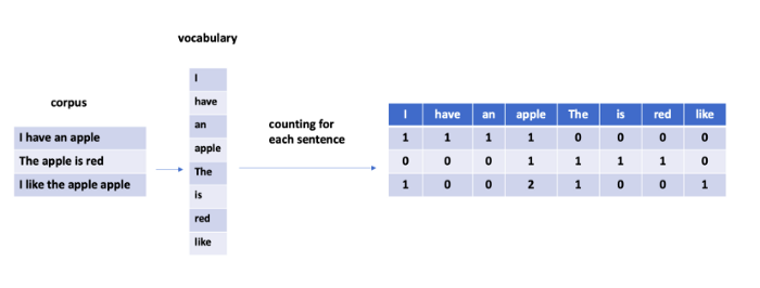
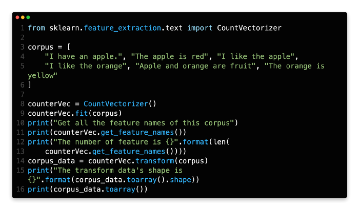
You need to extract the corpus between lines 3 and 5.
A CountVectorizer object can be created in line 8. This object is then fitted to the corpus at line 9.
In line 11, you would see the names of all features. The feature in this example is the word itself.
When the corpus is transformed at line 14, the output of line 16 is only a matrix with zeros and ones.
By using CountVectorizer, extract bigrams
Previously, only unigrams were used as features. By passing ngram_range=(1, 2) to the constructor, we can try both unigrams and bigrams:
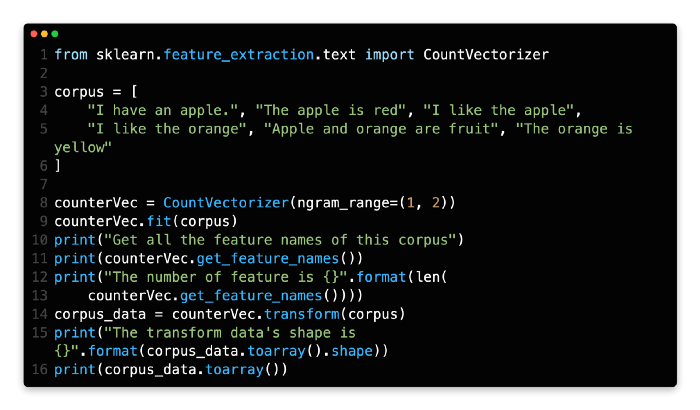
A corpus is a set of data that needs to be extracted between lines 3 and 5.
In line 8, you will find a description of how to create a CountVectorizer object. In the following example, we pass the parameter ngram_range=(1, 2), which means that the unigrams and bigrams in this demo will both be extracted.
I can see that the word pairs like apple is, and are fruits from the output of the get_feature_names function at line 11. Bigrams are what they are called. There are now 25 features on the feature list, which is an increase from 20 previously.
Missing Value
There are a lot of missing values in real datasets. There may be blanks, nan, inf, or other specified values in the datasets due to a variety of reasons. Some normal values, such as 0 and 1, are also considered missing values. Missing values: why do we care?
Missing values cannot be handled by some algorithms or implementations. The dataset is assumed to be complete.
We would have to adjust our model to account for the missing values.
Most of the time, the first reason is the main one.
If there are too many missing values in a row or column, you may want to consider just dropping them. It’s a good idea to drop only a small portion of the data. Dropping large amounts of data can, however, cause other problems. Dropping the whole column, for example, results in the loss of information. It can also be imputed. Missing value imputation can be achieved with sklearn functions.
Simple method of imputation
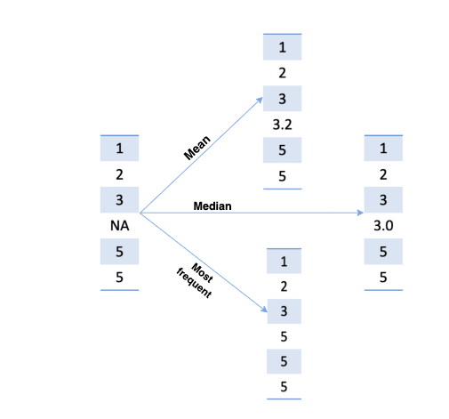
In the SimpleImputer, missing values are imputed using simple strategies.
Each column should be replaced with the mean of the missing values.
The median should be used to replace missing values along each column.
The most frequent value in each column should be replaced with the missing value. Numeric and string data can both be processed this way.
A constant value can be used to replace missing values.
There is another parameter, missing_values, which lets you specify which values to consider missing. Missing values have defaulted to np.nan.
Let’s start by creating a matrix and filling some values as np.nan.
import numpy as np

np.random.seed(42)
X = np.random.random(size=(4, 4))
## set the missing value
X[2, 3] = np.nan
X[3, 0] = np.nan
Next, let’s imput the missing value based on its mean. A simple imputer is created by SimpleImputer. Use strategy=’mean’ to specify the strategy, and fit_transform to transform the original data.
from sklearn.impute import SimpleImputer

imp_mean = SimpleImputer(strategy='mean')
# X is your original data matrix
X_mean = imp_mean.fit_transform(X)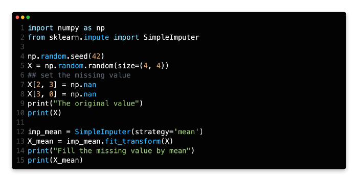
Creating a random matrix starts at line 5 and ends at line 8. In the meantime, some locations have been set to NaN.
Line 12 creates a SimpleImputer object using the mean imputation strategy. Line 13 transforms the original matrix.
At line 15, you can see the result.
KNN imputation
For filling in the missing values, SkLearn provides a function called KNNImputer. The k-Nearest Neighbor function is used to impute missing values. Using n_neighbors nearest neighbors found in the training set, missing values are imputed for each sample. SimpleImputer uses a similar approach.
The parameter n_neighbors is set to 3 in the example below.
from sklearn.impute import KNNImputer

knn = KNNImputer(n_neighbors=3)
X_trans = knn.fit_transform(X)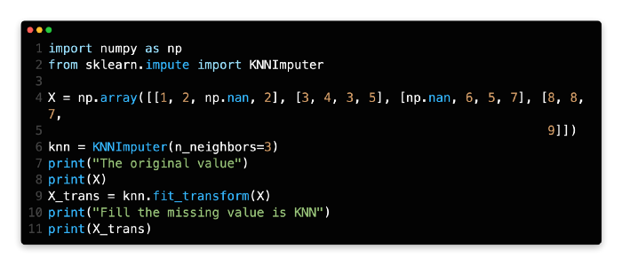
Line 4 creates a dataset.
A KNNImputer object is then created at line 6. The k for KNN is set in this example to 3 by setting n_neighbors=3.
Metrics
The importance of metrics in Machine Learning tasks cannot be overstated. Defining a Machine Learning task requires defining which metrics you will evaluate. Machine Learning models should be evaluated for their performance. Metrics provide you with information about the performance of your model. It can be even more problematic if you choose the wrong metrics.
For this reason, defining an appropriate evaluation index for Machine Learning is crucial.
We usually have some recognized metrics for supervised learning. Different metrics are used for classifying and regressing problems. The same types of tasks, such as classification tasks, can be evaluated in a variety of ways, such as using F1-scores, AUCs, accuracy, etc. There are some metrics that can be used in any situation, and there are some that can only be used in certain scenarios.
The situation is more complicated for unsupervised learning, and the metrics vary widely for different tasks. Clustering metrics, for example, are not as universal as those used in supervised learning.
There are many functions available in SkLearn that cover a wide range of tasks and scenarios.
Classification
Confusion matrix
Defining some terms used in binary classification tasks is important before we discuss the confusion matrix.
In the data, P represents the number of real positive cases.
In the data, N represents the number of negative cases.
It is a true positive if both the prediction result and the actual result are positive.
Negative results in True Negatives: both the prediction and real values are negative.
FP: False Positive: The prediction is positive, but the actual value is negative.
False Negative: the prediction results in a negative value, but the real value is positive.
There are two rows and two columns in the confusion matrix, which report the number of false positives, false negatives, and true positives.
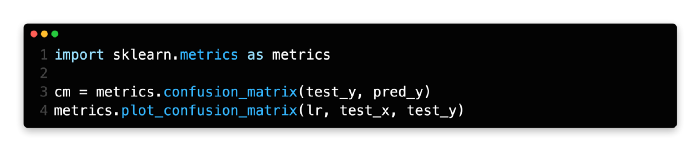
A matrix can be output using the sklearn function. Furthermore, the matrix can be plotted in color using this program.
Based on the true label and the predicted label, the confusion matrix is calculated with the confusion_matrix. The confusion matrix is plotted as a heatmap using plot_confusion_matrix. Below is one example of a confusion matrix plot.
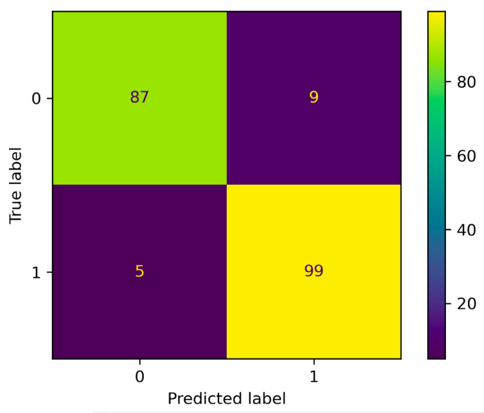
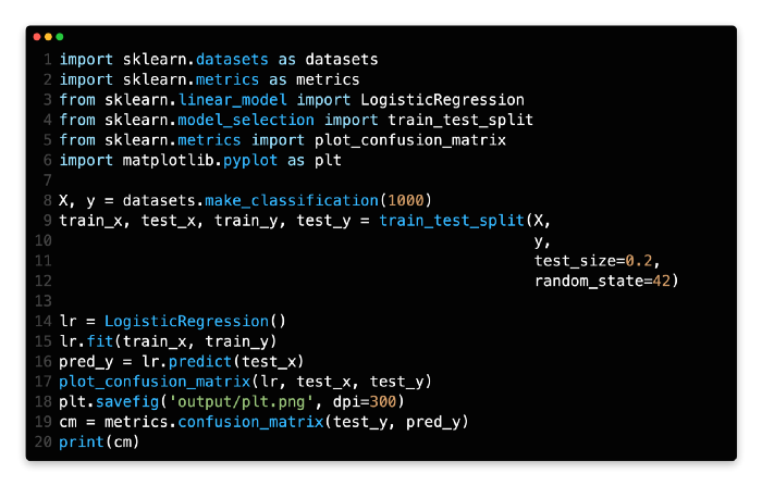
The binary classification dataset is generated from line 6 to line 10 and split into two parts. Eighty percent of the binary classification dataset is contained in the training set.
Using LogisticRegression(), a logistic regression model is created and trained from line 12 to line 13.
The test dataset is predicted using the model at line 14.
The confusion matrix is calculated using confusion_matrix() in line 15. Both the ground truth test_y and the prediction pred_y must be passed.
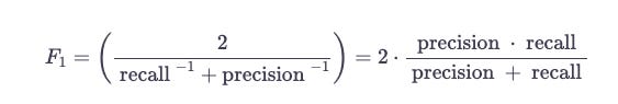
F1-score
F1 scores are used to measure the accuracy of binary classification tests. In addition to precision, it also considers pp and the recall rr. The score is calculated based on the results of the test. Precision and recall are combined to form the harmonic mean of F1.
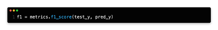
It is the f1_score function that you need. The true Y and prediction Y should be passed as follows.
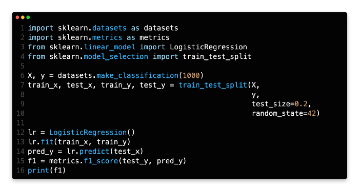
The binary classification dataset is generated from lines 6 to 10 and split into two parts. There are 80% of the binary classification datasets in the training set.
Lines 12 and 13 create and train a logistic regression model from LogisticRegression().
The model is used to make predictions on the test dataset at line 14.
In line 15, you can see how to calculate f1_score using f1_score(). A prediction pred_y and a ground truth test_y need to be passed.
AUC
Let’s spend a few minutes talking about ROC before we get to AUC. As a binary classifier system’s discrimination threshold is varied, a receiver operating characteristic curve can illustrate its diagnostic ability. The ROC curve is simply the plot of the true positive rate (TPR) against the false positive rate (FPR) at various threshold levels.
Normalized units specify the probability that a classifier will rank a positively ranked instance higher than a negatively ranked instance by the area under the curve. When the ratio of positive to negative samples is unbalanced, AUC is often used to measure classifier performance.
Let’s see how to calculate the AUC. In order to calculate the AUC, we need a series of TPR and FPR since the ROC curve is based on TPR and FPR.
fpr, tpr, thresholds = metrics.roc_curve(test_y, pred_y)
auc = metrics.auc(fpr, tpr)
Sklearn offers a function that can be used to draw an ROC curve, as shown below. Model evaluation is the first parameter. It’s a Logistic Regression in this example. Once the test samples and labels are passed, we can proceed.
metrics.plot_roc_curve(lr, test_x, test_y)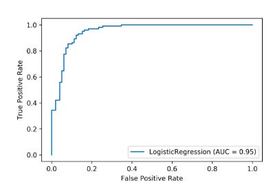
Classification report
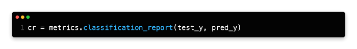
The classification_report function provided by Sklearn provides a useful overview of the main classification metrics.’
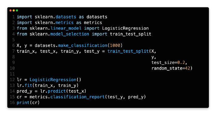
The binary classification dataset is generated from line 6 to line 10 and then split into two parts. There are 80% of binary classification datasets in the training set.
As a result of LogisticRegression(), a logistic regression model is created and trained on lines 12 and 13.
At line 14, we predict the results based on the model.
The function classification_report() can be used to output some classification metrics, such as precision, recall, and f1. Pred_y (line 14 output) and test_y (ground truth) must be passed.
Regression
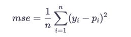
There are fewer metrics in regression compared to classification. The most common one is MSE. If p_{i}pi is the predicted value, and y_{i}yi is the true value for i-th instance, then:
mse = metrics.mean_squared_error(test_yr, pred_yr)Below is the complete code, you can have a try.
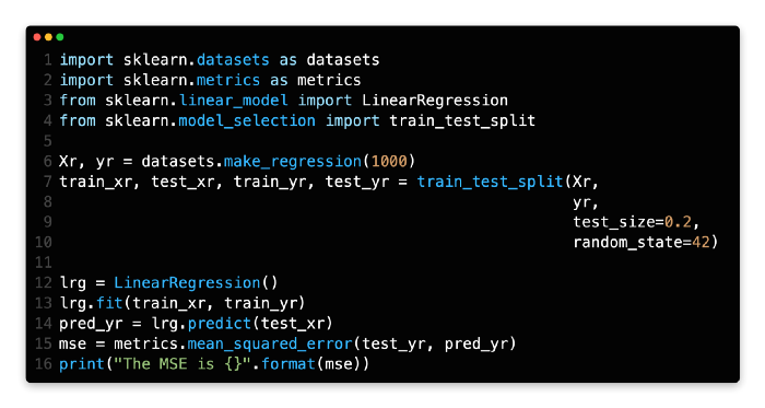
There are two parts to the regression dataset generated from line 6 to line 10. 80% of the regression dataset is contained in the training set.
A linear regression model is created from LinearRegression() and trained from line 12 to line 13.
On line 14, we predict the test dataset using the model.
MSE can be calculated using mean_squared_error() on line 15. A prediction pred_yr (line 14’s output) and a ground truth test_yr must be passed.
Parameter Searching
A Machine Learning project requires fine-tuning parameters, especially when it comes to Deep Learning. It is important to note that even though this course focuses on traditional Machine Learning, the parameter space is limited and a few parameters need to be adjusted. Some models, such as tree-based models, still require a lot of parameters.
In practice, fine-tuning is done by hand. A series of parameters is tested, models are evaluated, and the best one is chosen. Once all parameters have been chosen, the process is repeated if there are more than two parameters. This is a time-consuming and tedious process that can be automated completely.
We can use some useful functions provided by Sklearn. We will only focus on GridSearchCV in this lesson. Other aspects of the principle are similar.
Grid Search
In GridSearchCV, the param_grid parameter is used to generate an exhaustive grid of candidate values. Using the tree-based model in this example, we have a lot of parameters to consider.
We’ll skip the loading and splitting of data and go straight to building the model and searching for parameters.
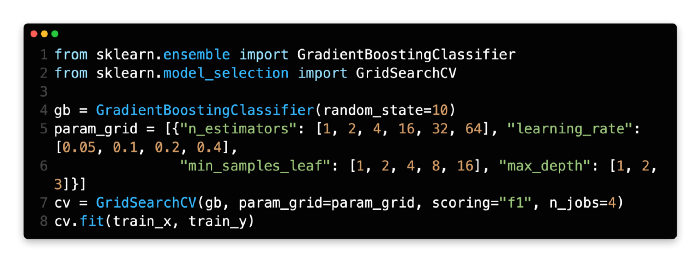
To fine-tune the estimator, let’s create it first. This example involves creating a GBDT classifier. Then, we define a parameter_grid map. A GridSearchCV object is then created and fitted. We set n_jobs=4 to enable multiple processors to speed up training; it may take 30 seconds. You can figure out the number of combinations from the param_grid above 6 * 5 * 4 * 3 = 3606∗5∗4∗3=360. In other words, the GridSearchCV would train and evaluate 360 models. GridSearchCV, therefore, is a very inefficient approach. The process can save you a great deal of time and effort if there is a small amount of data to process.
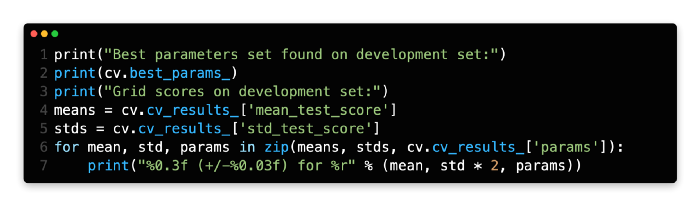
There are some useful attributes in the GridSearchCV object. The best parameter can be obtained by using the best_parameter_ attribute. Cv_results_ also provides the evaluation metrics for each set of parameters.
You can have a look at the complete code here.
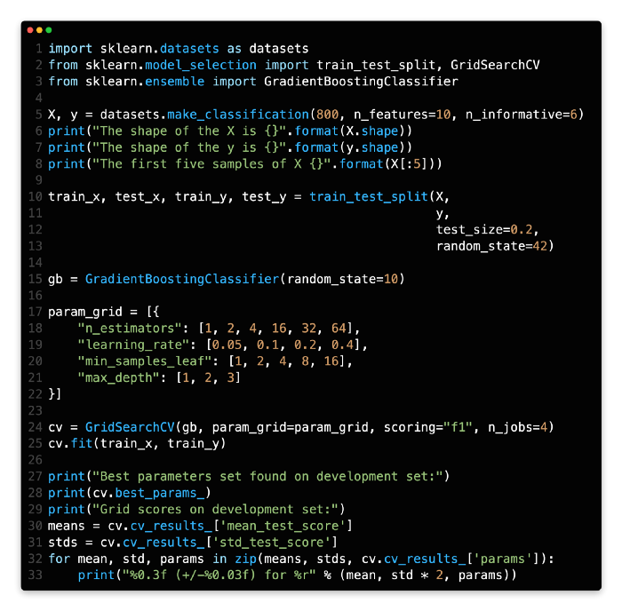
As a first step, we will create a dataset called make_classification at line 5, which will have a size of 800 * 10.
Line 10 divides the dataset into two sections, the train set and the test set. The training set accounts for 80% of the dataset.
As our model, we are using the GBDT. Therefore, line 15 creates a GBDT.
We are trying to finetune the parameters from lines 17 to 22 of the param_grid dictionary.
The GridSearchCV object is created at line 24. The f1-score is used as the metric in this example.
We can determine the best parameter by looking at the output of line 28. The cv_results_ file also contains all parameters and their corresponding metrics.
