


Harnessing Arbitrage Opportunities in Dual Exchange Trading
Harnessing Arbitrage Opportunities in Dual Exchange Trading
Developing a Python-Based Algorithm to Capitalize on Price Discrepancies Between Stock Exchanges

A Project to identify arbitrage opportunities between two stock exchanges trading the same stock. The algorithm searches for the possibility of a mismatch and trades on it. Next to that, it takes into account certain limits, which is set to a max position of 250 to prevent massive losses if the algorithm malfunctions.
# Import pandas and numpy for analysis
import pandas as pd
import numpy as np
import matplotlib.pyplot as plt

# Set Jupyter to render directly to the screen
%matplotlib inline
Code snippets provide Python environments with data analysis and visualization libraries. The program imports the pandas library under the alias pd, commonly used to read in data files, clean data, group data and agglomerate it. Numpy is imported with the alias np, which supports arrays and matrices, and is primarily used as a numerical computing library. Aside from that, the code imports the pyplot module from the matplotlib library under the alias plt. In Python, this module creates static, interactive, and animated visualizations including graphs and charts. The final line %matplotlib inline generates a magic command for IPython-based interfaces, such as Jupyter notebooks. In this command, the environment is modified so that Matplotlib plots can be displayed directly in the notebook. This allows graphs and figures to be rendered inline, directly under the code cells where plotting commands are executed, for quick visualization and analysis of data.
def read_data(filename):
    '''
    This reads the .csv stored at the 'filename' location and returns a DataFrame
    with two-level columns. The first level column contains the Exchange and the
    second contains the type of market data, e.g. bid/ask, price/volume.
    '''
    df = pd.read_csv(filename, index_col=0)
    df.columns = [df.columns.str[-7:], df.columns.str[:-8]]

    return df
In the code, a function named read_data is defined. It requires one parameter, filename, which represents the path to a CSV file. The function uses the pandas library (implied by the pd shorthand) to read this CSV file into a DataFrame object. A specific manipulation is then performed on the columns of this DataFrame: it splits each column name into two levels for multi-level indexing, where the first level is the last seven characters of the column name, and the second level is the remainder excluding the last eight characters of the column name. In order to make this splitting meaningful, the CSV files column names must be formatted in such a way that it results in meaningful categorization for the Exchange and market data type. The function returns the modified DataFrame after formatting the columns. An efficient way to access hierarchical data within the DataFrame could be achieved by utilizing this multi level index.
# Read the data for one of the stocks
filename = 'HWG.csv'
market_data = read_data(filename)
This code snippet is used to load data from a CSV file called HWG.csv. The file contains market data for a stock that is presumably represented by it. The first line is a comment that is ignored by the Python interpreter and is only there for human readers to understand. Using the string HWG.csv as its argument, the function read_data is called in the second line, which uses string filename as its argument. This snippet does not define the read_data function, so it must be defined elsewhere in the code or imported. Data will be read from the file HWG.csv and returned by the function. Data returned is then stored in the variable market_data. We can assume, without knowing the details of the implementation, that read_data is designed to return structured market data by processing and parsing the CSV file. The code lets the user load and possibly preprocess market data related to stocks, which can then be used for analysis, visualization, and trading algorithms, as well as other operations as part of the larger program.
# Visualization of the columns in the DataFrame
market_data.head()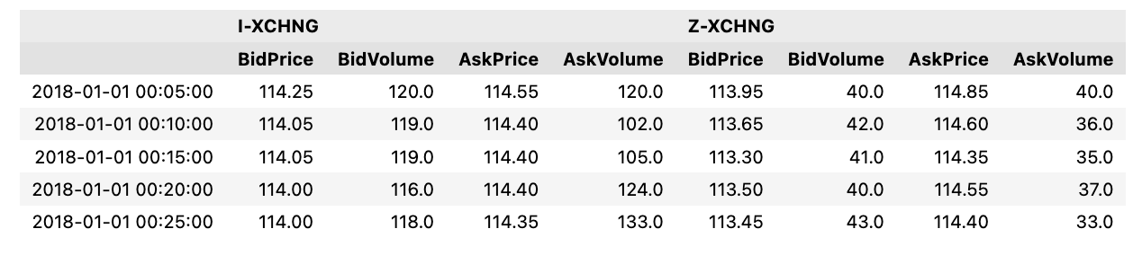
As you can see, the code displays the first few entries (typically the first five) of the DataFrame named market_data for the purpose of visual inspection. In the context of data analysis, the .head() method is used to quickly get a sense of what data is contained in the DataFrame, the structure of the data, and to confirm that the data has been loaded correctly. A large dataset cannot be displayed in full using this method.
# Select the first 250 rows
market_data_250 = market_data.iloc[:250]

# Set figsize of plot
plt.figure(figsize=(16, 10))

# Create a plot showing the bid and ask prices on different exchanges
def Plot_Bid_Ask(stock1 = 'I-XCHNG', stock2 = 'Z-XCHNG'):
    plt.plot(market_data_250.index, market_data_250[stock1, 'BidPrice'])
    plt.plot(market_data_250.index, market_data_250[stock2, 'AskPrice'])
    plt.xticks([])
    plt.xlabel('Time')
    plt.ylabel('Price')
    plt.title('Bid Price on '  + stock1 + ' vs Ask Price on ' + stock2)
    plt.legend([stock1 + ' BidPrice', stock2 + ' AskPrice'])
    plt.show()


# Note arbitrage possible in case the BidPrice is higher than the AskPrice.
Plot_Bid_Ask()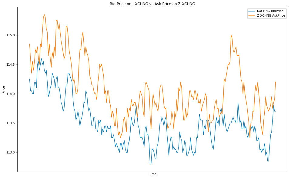
A new variable called market_data_250 is created by selecting the 250 first rows of a dataset called market_data. A plot of 16 inches by 10 inches is created by using plot.figure(figsize=(16, 10)). Using this function, the parameters specify two different exchanges labelled I-XCHNG and Z-XCHNG. In the example, a bid line is plotted, using data from stock_market_data_250, and an ask line is plotted, using data from stock_market_data_250. To omit showing actual values, it uses empty ticks for the x-axis, sets labels for the axes, and adds a title that changes depending on the exchanges being compared. Plot lines are identified by legends. This function produces a plot using the default exchanges specified in the function definition when called without any arguments. Additionally, the code indicates that there is an opportunity for arbitrage (profiting from price differences) whenever the bid price exceeds the ask price.