


Harnessing Deep Reinforcement Learning for Algorithmic Trading
Harnessing Deep Reinforcement Learning for Algorithmic Trading
Predicting stocks using deep reinforcement learning, time series.

In the ever-evolving world of finance, the stock market has always been an exciting realm for investors, traders, and enthusiasts alike. With the rapid transition from traditional, face-to-face stock exchanges to digital platforms, the landscape has dramatically transformed, opening up new opportunities and challenges for investment companies and individual traders. As we stand on the precipice of yet another technological revolution, it is crucial for stock market aficionados to stay ahead of the curve, understanding and embracing the potential of cutting-edge approaches like deep reinforcement learning in algorithmic trading.
This article aims to delve into the fascinating world of algorithmic trading, exploring how deep reinforcement learning can revolutionize the way we approach the dynamic and complex stock market. Geared towards those with a keen interest in stocks, trading, and time series analysis, we will examine the limitations of traditional trading strategies and introduce the concept of treating the trading process as a Markov Decision Process (MDP). This fresh perspective, combined with the power of reinforcement learning algorithms, promises to maximize portfolio returns and uncover the best trading strategies even in the face of unpredictable market crashes.
Now let’s start with import statements.
Imports
!pip install yfinance
!pip install ta
!pip install stable.baselines3
!pip3 install torch torchvision torchaudio

#!pip install TA-Lib
import warnings
import yfinance
import pandas as pd
import numpy as np
import matplotlib.pyplot as plt
import seaborn as sns
import datetime
import ta
import os
#import talib
warnings.filterwarnings("ignore")
# Optional Plotly Method Imports
import plotly
import cufflinks as cf
cf.go_offline()


from stable_baselines3 import A2C, PPO, DDPG
from stable_baselines3.common.policies import ActorCriticPolicy #MlpPolicy for A2C and PPO
from stable_baselines3.td3.policies import MlpPolicy
from stable_baselines3.common.vec_env import DummyVecEnv, VecNormalize
from stable_baselines3.common.evaluation import evaluate_policy
from stable_baselines3.common.noise import ActionNoise, OrnsteinUhlenbeckActionNoise

sns.set_style('whitegrid')
%matplotlib inline
Throughout the project, this code installs several packages. The !pip install commands install the following packages:
You can download historical stock prices from Yahoo Finance API using yfinance.
A package that gives you technical analysis indicators for financial data.
Stable.baselines3: Algorithms for reinforcement learning.
PyTorch deep learning packages torch, torchvision, torchaudio.
Importing the warnings package suppresses any warning messages that may appear.
Data manipulation and visualization are done with pandas, numpy, matplotlib, and seaborn.
You can work with dates and times with the datetime package.
File paths can be checked with the os package.
For optional interactive visualizations, plotly and cufflinks packages are imported.
It imports A2C, PPO, DDPG, ActorCriticPolicy, MlpPolicy, DummyVecEnv, VecNormalize, evaluate_policy, and OrnsteinUhlenbeckActionNoise from the stable_baselines3 package. Jupyter notebooks can plot inline using %matplotlib inline and sns.set_style().
Data Collection
#DJIA stocks
tic = ['MMM', 'AXP', 'AMGN', 'AAPL', 'BA', 'CAT', 'CVX',
       'CSCO', 'KO', 'DOW', 'GS', 'HD', 'HON', 'IBM', 'INTC',
       'JNJ', 'JPM', 'MCD', 'MRK', 'MSFT', 'NKE', 'PG', 'CRM',
       'TRV', 'UNH', 'VZ', 'V', 'WBA', 'WMT', 'DIS' ]
As of September 2021, this code creates a list called tic with the tickers for the 30 Dow Jones Industrial Average (DJIA) companies. There are different ticker symbols for different companies listed on the exchange. There are 30 large, publicly traded companies in the United States that make up the DJIA. Using the yfinance package, you can retrieve data from Yahoo Finance API using ticker symbols.
stock_data = pd.DataFrame()
stock_start_date = '2009-01-01'
stock_end_date = '2021-07-01'

for s in tic:

  temp_data = yfinance.download(s, start= stock_start_date, end=stock_end_date)
  temp_data['Ticker'] = s

  stock_data = stock_data.append(temp_data)
In this code, we create a pandas DataFrame called stock_data and use yfinance.download() to download historical stock data. Using the yfinance.download() function with the specified start and end dates, the code retrieves historical stock price data from Yahoo Finance API for each stock ticker symbol in the ticker list. Temporary DataFrame temp_data stores the downloaded data.
To identify the stock associated with each row of data, the Ticker column has the ticker symbol of the current stock. After that, the temp_data DataFrame is appended to the stock_data DataFrame, combining all the historical stock price data for all the stocks in the ticker.
All 30 stocks in the DJIA from January 1, 2009 to July 1, 2021 will be in stock_data at the end of the loop.
Data Exploration
stock_data.head()
The first five rows of the stock_data DataFrame will be displayed when you call stock_data.head(). Depending on the date range, the output will show the date, opening price, highest price, lowest price, closing price, volume, and adjusted closing price (Adj Close). There will also be a Ticker column that shows the stock associated with each row.
Below are the first five rows of the stock_data DataFrame for the 3M Company stock (MMM), including the date, opening price, highest price, lowest price, closing price, volume, and adjusted closing price.
stock_data.Ticker.unique()
In the Ticker column of the stock_data DataFrame, this code returns an array of unique ticker symbols. This method returns an array of unique ticker symbols in the specified column of the DataFrame.
Especially if there are a lot of stocks being analyzed, this code is useful for making sure all the expected stocks are there. A dataframe containing the stock prices of all the companies whose stock tickers are in the stock_data DataFrame will be output.
plt.figure(figsize=(10,5))
stock_data.groupby(by= 'Ticker').count()['Open'].plot(kind = 'bar')
plt.xlabel('Ticker', fontsize = 12)
plt.ylabel('Unique Trading Days', fontsize = 12)
plt.title('Box Plot showing Unique Trading Days per Stock', fontsize = 14)
plt.show()
This code displays the number of unique trading days for each stock in the stock_data DataFrame using the matplotlib library. For each group (in other words, each stock), we use the groupby() method to group the DataFrame by the Ticker column, and we use the count() method to count how many unique values there are in the Open column.
Each ticker symbol is represented on the x-axis, with the resulting counts plotted as bars. You can add labels to the x-axis, y-axis, and title of the plot using plt.xlabel(), plt.ylabel(), and plt.title() functions.
This plot helps identify missing or incomplete data for individual stocks by visualizing the number of trading days for each stock in the DJIA. Figure size is set with figsize, and the plot is displayed with plt.show().
#EDA
df = stock_data.copy()
# Dropping Closing Price Column
df = df.drop('Close', 1)
df = df.drop('Open', 1)
df = df.drop('High', 1)
df = df.drop('Low', 1)
df = df.drop('Volume', 1)
#Remanimg Adj Close
df = df.rename(columns={'Adj Close':'AdjClose'})
df = df.sort_values(by= ['Date', 'Ticker'])
df = df.reset_index()
df = df.pivot(index= 'Date', columns= 'Ticker')
df = df.droplevel(0, axis=1)
df = df.fillna(0)
To prepare the stock_data DataFrame for exploratory data analysis (EDA), this code does some data cleaning and reformatting.
By using the copy() method, we make a copy of stock_data DataFrame and assign it to df. Using the drop() method, we drop the columns for opening price, closing price, highest price, lowest price, and volume from the DataFrame, which indicates that columns should be dropped rather than rows.
For consistency, the Adj Close column is renamed to AdjClose with the rename() method. Using the sort_values() method, the DataFrame is sorted by date and stock ticker, and the index is reset.
Using pivot(), the DataFrame is reshaped into a wide format, with each ticker symbol represented by a separate column. To finish, we use the droplevel() method to remove the extra level of column indexing caused by the pivot, and we use the fillna() method to fill in any missing values.
EDA will now be able to work with a new DataFrame that has one row for each trading day and one column for each stock ticker symbol in the DJIA.
for i in range(5,35, 5):
  df.iloc[:,(i-5):i].plot(kind = 'line', figsize = (15, 8),  fontsize = 12)
  plt.xlabel('Date [Year]', fontsize = 12)
  plt.ylabel('Stock Price [$]', fontsize = 12)
  plt.legend(loc = 'best', fontsize = 12,title = 'Ticker', title_fontsize = '12')
  plt.title('Variation of Stock Price [2009 - 2021]', fontsize = 14)
  plt.show()
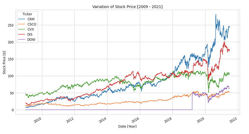
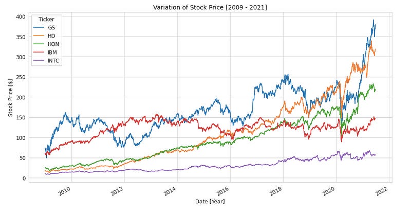
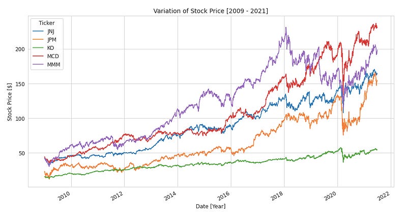
The code creates five line plots using the matplotlib library to show stock price variation for each stock in the DJIA over the specified time period, five stocks at a time. Each group of 5 stocks is selected using the iloc method, and a line plot is created using the plot() method.
You can add labels to each plot’s x-axis, y-axis, legend, and title using plt.xlabel(), plt.ylabel(), plt.legend(), and plt.title() functions. Figsize sets the figure size in inches, and fontsize sets the axis labels and legend font size.
Using this code, you can visualize the DJIA’s stock prices over time and identify stocks that have changed significantly in price or volatility over the specified period. Five line plots will be generated, each showing the variation in stock prices over time for five DJIA stocks.
 for idx in tic:
  plt.figure(figsize=(12,6))
  df[idx].loc['2009-01-01':].plot(label = '{} Close'.format(idx))
  df[idx].loc['2009-01-01':].rolling(window=63).mean().plot(label='Quarterly Avg')
  df[idx].loc['2009-01-01':].rolling(window=252).mean().plot(label='Yearly Avg')
  plt.xlabel('Date [Year]', fontsize = 12)
  plt.ylabel('Stock Price [$]', fontsize = 12)
  plt.legend(loc = 'best', fontsize = 12)
  plt.title('Closing Price vs Quarterly Average of {}'.format(idx), fontsize = 14)
  plt.show()
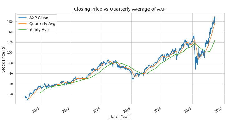

The code displays the closing price of each stock in the DJIA, along with rolling averages for each stock over a quarterly and yearly period using the matplotlib library. It sets the figure size for each plot with plt.figure().
The plot() method creates a line plot of each stock’s closing price, along with rolling averages calculated using the rolling() method with window values of 63 (for quarterly averages) and 252 (for yearly averages). Each plot line is labeled with the label parameter using the loc[] method, which selects data starting on January 1, 2009.
You can add labels to the x-axis, y-axis, legend, and title of each plot using plt.xlabel(), plt.ylabel(), plt.legend(), and plt.title(). Axis labels and legends are sized by the fontsize parameter.
Using this code, you can visualize the closing price trend over time for each stock in the DJIA, as well as identify long-term trends or seasonal patterns. Each line plot will show the closing price and rolling average for one DJIA stock.
plt.figure(figsize=(20,10))
sns.heatmap(df.corr(), annot=True)
This code visualizes pairwise correlations between the columns of the df DataFrame using the seaborn library. The plt.figure() function sets the heatmap’s figure size.
Heatmaps of correlations between columns are created using the sns.heatmap() function. By setting annot=True, each cell in the heatmap gets the correlation coefficient.
It can help inform portfolio allocation decisions by identifying strong correlations between closing prices of different stocks in the DJIA. It’ll be a heatmap with each cell representing a correlation coefficient between two stocks, with brighter colors representing stronger correlations.
Data Pre-Processing
# Dropping Closing Price Column
stock_data = stock_data.drop('Close', 1)

#Remanimg Adj Close
stock_data = stock_data.rename(columns={'Adj Close':'AdjClose'})

#Resetting the index
stock_data = stock_data.reset_index()

#Sorting the data by Date and Ticker and resetting the index
stock_data = stock_data.sort_values(by= ['Date', 'Ticker']).reset_index(drop = True)
The stock_data DataFrame gets cleaned up and reformatted in this code.
By passing 1 as the second argument to the drop() method, the closing price column is dropped from the DataFrame (as opposed to rows).
For consistency, the Adj Close column is renamed to AdjClose using rename().
Using the sort_values() method, we sort the DataFrame by date and stock ticker, and reset the index with reset_index(). Dropping the old index column and creating a new one is done with the drop parameter set to True.
With these operations, you get a new DataFrame, which has one row for each trading day and one column for each relevant feature, such as adjusted closing price, opening price, high, low, and volume.
# Feature Engineering
# Extracting features from date column

stock_data['Day'] = stock_data['Date'].dt.dayofweek
stock_data['Week'] = stock_data['Date'].dt.week
stock_data['Month'] = stock_data['Date'].dt.month
In this code, the Date column is used to create new features on the stock_data DataFrame. To create three new features, we use the dt attribute to access the Date column’s date components:
An integer representing the day of the week, with Monday being 0 and Sunday being 6
An integer representing the week number of the year
An integer representing the month of the year
The new features could help us identify additional patterns or trends in the data based on the time of year or day of the week.
The Date column must already be formatted as a datetime object for this approach to work. Date columns may need to be converted first to datetime objects using pd.to_datetime() if they’re currently strings.
uniq_date = stock_data.Date.unique()
stocks = pd.DataFrame({"Date": uniq_date})

stock_data_tech = pd.DataFrame()

#Make changes first calculate the technical indicators and then match all the stocks with dates and then backfill NaN with last observed valid data
for i in tic:

  #Forcing all all the date ranges to be same for all stocks #DOW
  temp = pd.merge(stocks, stock_data[stock_data.Ticker == i], how='left', on= 'Date')

  #Filling the missing values
  temp = temp.fillna(method='bfill')

  print('Shape of {} before merging : {} | after merging : {}'.format(i, stock_data[stock_data.Ticker == i].shape, temp.shape))

  #Adding all the available technical indicators
  stock_tech = ta.add_all_ta_features(df= temp, open= 'Open', high= 'High', low= 'Low', close='AdjClose', volume = 'Volume', fillna=True)

  stock_data_tech = stock_data_tech.append(stock_tech)
Using the Date column of the stock_data DataFrame, this code creates a new DataFrame stocks. To store the technical indicators that will be calculated for each stock, we create a new DataFrame stock_data_tech.
For each stock ticker, a loop iterates over it and performs the following steps:
Use the pd.merge() method to merge the stocks DataFrame with the subset of the stock_data DataFrame that corresponds to the current stock. No matter if the current stock has data for that date or not, all rows in the resulting DataFrame will have the same dates.
Use the fillna() method with the bfill parameter to fill in any missing values in the DataFrame. Fill in any missing values with the last valid observation.
The ta library has a function ta.add_all_ta_features() for adding technical indicators. By using this function, you can calculate moving averages, RSI, Bollinger Bands, and other technical indicators, and add them to your DataFrame. It fills in any missing values with the column mean.
Use the append() method to append the resulting DataFrame to the stock_data_tech DataFrame.
Using this approach, you’ll get a new DataFrame that includes both the original stock price data and newly calculated technical indicators.
stock_data_tech[['Date', 'Ticker', 'Open', 'High', 'Low', 'AdjClose', 'Volume','momentum_ppo', 'momentum_rsi','trend_adx', 'trend_macd', 'trend_cci' ]].sample(5)
Using the indexing operator [] and a list of column names, this code selects a subset of columns from the stock_data_tech DataFrame. These are the columns I selected:
Date: The date of the trading day
Ticker: The stock ticker
Open: The opening price of the stock on the trading day
High: The highest price of the stock on the trading day
Low: The lowest price of the stock on the trading day
AdjClose: The adjusted closing price of the stock on the trading day
Volume: The volume of shares traded on the trading day
momentum_ppo: The percentage price oscillator, which is a technical indicator that measures momentum
momentum_rsi: The relative strength index, which is a technical indicator that measures momentum
trend_adx: The average directional index, which is a technical indicator that measures trend strength
trend_macd: The moving average convergence divergence, which is a technical indicator that measures trend strength
trend_cci: The commodity channel index, which is a technical indicator that measures trend strength
Using the sample() method, five rows are randomly selected from the resulting DataFrame to provide a sample.
Custom Trading Environment
class StockTradingEnv(gym.Env):
    metadata = {'render.modes': ['human']}

    def __init__(self, df, Shares_Per_Trade = 10, Initial_Investment = 10000, Action_Space = 30, Observation_Space = 211, day = 0,
                 Normalized_Rewards = 1e-4, verbosity = 0, mode = 'train', seed = 10, commission = 0 ):

      self.day = day
      self.df = df
      self.max_shares_per_trade = Shares_Per_Trade
      self.initial_investment = Initial_Investment
      self.Action_Space = Action_Space
      self.Observation_Space = Observation_Space
      self.normalized_rewards = Normalized_Rewards
      self.verbosity = verbosity
      self.commission = commission
      #self.model = model
      self.mode = mode
      self._seed(seed)


      #Action Space
      # Action > 0  means buy shares of stock
      # Action 0 means Hold the stock
      # Action < 0 means sell shares of stock
      self.action_space = spaces.Box(low = -1, high= 1,
                                     shape=(self.Action_Space,), dtype= np.int)

      #Observation Space
      self.observation_space = spaces.Box(low = -np.inf, high= np.inf, shape=(self.Observation_Space,))

      #Selecting the Data for one date
      self.data = self.df.loc[self.day,:]

      #Initial Run
      self.initial = True

      #Verify if tradings days are completed or not
      self.done = False

      #Rewards
      self.reward = 0

      #Asset value after each trading day
      self.asset_memory = [self.initial_investment]

      #Rewards received for each trading day i.e profit or loss
      self.reward_memory = []

      #Saving the date for the trade
      self.date_memory = [self.data.Date.unique()[0]]

      #Initializing state of the environment

      self.state = [self.initial_investment] + self.data.AdjClose.values.tolist() + [0]*self.Action_Space + \
        self.data.momentum_ppo.values.tolist() + self.data.momentum_rsi.values.tolist() + \
        self.data.trend_adx.values.tolist() + self.data.trend_macd.values.tolist() + \
        self.data.trend_cci.values.tolist()


    def render(self, mode='human'):
      return self.state

    # This method is used to reset the values of the state to it's default after every episode
    def reset(self):

      self.day = 0
      self.reward = 0
      self.data = self.df.loc[self.day,:]
      self.done = False
      self.initial = False
      self.reward_memory = []
      self.date_memory = [self.data.Date.unique()[0]]
      self.asset_memory = [self.initial_investment]
      self.state = [self.initial_investment] + self.data.AdjClose.values.tolist() + [0]*self.Action_Space + \
        self.data.momentum_ppo.values.tolist() + self.data.momentum_rsi.values.tolist() + \
        self.data.trend_adx.values.tolist() + self.data.trend_macd.values.tolist() + \
        self.data.trend_cci.values.tolist()
      #print(self.state)
      return self.state

    def step(self, actions):
      self.done = self.day >= len(self.df.Date.unique())-1

      #Use this to save the results to csv after we performed trading for all the days
      if self.done:

        final_portfolio_value = self.state[0] + sum(np.array(self.state[1:self.Action_Space+1])*
                                                     np.array(self.state[self.Action_Space+1:(2*self.Action_Space)+1]))

        total_rewards = final_portfolio_value - self.initial_investment
        profit_pct = (total_rewards*100)/self.initial_investment

        asset_df = pd.DataFrame(self.asset_memory)
        asset_df.columns = ['portfolio']
        asset_df['date'] = self.date_memory

        if self.verbosity and self.mode != 'train':

          #print(len(self.reward_memory))
          #if self.mode == 'trade' or self.mode == 'val':
          print( 'Initial Portfolio Value : {} | Final Portfolio Value : {} | Total rewards : {} | % of profit : {}'.format(self.initial_investment, final_portfolio_value,total_rewards, profit_pct))
          asset_df.to_csv('{}_{}_results'.format(self.mode, self.commission))
        return self.state, self.reward, self.done, {}

      else:

        #Calculating the portfolio value before start of trading
        #Available investment amount + sum of value of each stock held (no.of shares per stock * price of the stock on that day)
        portfolio_before_trade = self.state[0] + sum(np.array(self.state[1:self.Action_Space+1])*
                                                     np.array(self.state[self.Action_Space+1:(2*self.Action_Space)+1]))

        #Extracting the indicies of sell action
        #if actions is not an array then convert it to array using np.array()
        sell_indices = np.where(actions <  0 )[0]

        #Extracting the indicies of buy action
        buy_indices = np.where(actions >  0 )[0]

        ###### Trading starts #######
        # Initially selling the stocks to increase investment value
        for idx in sell_indices:
          #Sell stock if price is > 0 and shares held > 0

          if self.state[idx+1] > 0 and self.state[idx+self.Action_Space+1] > 0:

            #No of shares to sell
            shares_sell = min(self.state[idx+self.Action_Space+1], abs(actions[idx]*self.max_shares_per_trade))

            #Updating the available cash after selling the stocks
            self.state[0] += self.state[idx+1]*shares_sell*(1-self.commission)

            #Updating the available stocks after selling
            self.state[idx+self.Action_Space+1] -= shares_sell

          else:
            # print('No Shares to sell')
            pass

        #print('Buying Stock shares : ')
        for idx in buy_indices:
          #Buy stocks if price is > 0

          if self.state[idx+1] > 0 and self.state[0] > 0:

            #Max number of shares that can be brought with the available cash (available cash / stock price)
            max_shares_buy = self.state[0]*(1 - self.commission)//self.state[idx+1]

            #No of shares to buy
            shares_buy = min(max_shares_buy, actions[idx]*self.max_shares_per_trade)

            #Updating the available cash after selling the stocks
            self.state[0] -= self.state[idx+1]*shares_buy*(1 + self.commission)

            #Updating the available stocks after selling
            self.state[idx+self.Action_Space+1] += shares_buy

          else:
            # print('No Shares purchased')
            pass

        ###### Trading ends #######
        # print('*************** Trading Ends ***************')
        # print('Available cash for after trading : {}'.format(self.state[0]))
        # print('Shares available per stock : '.format(np.array(self.state[self.Action_Space+1:(2*self.Action_Space)+1])))
        # print('Over all portfolie before Trading : {}'.format(portfolio_after_trade))
        # print('Profit or Loss for Day {} : {} is {}'.format(self.day, self.date_memory[-1], self.reward))

        #Setting the values for next trading date
        self.day += 1
        self.data = self.df.loc[self.day,:]

        self.state = [self.state[0]] + self.data.AdjClose.values.tolist() + list(self.state[(self.Action_Space+1):(2*self.Action_Space)+1]) + \
                      self.data.momentum_ppo.values.tolist() + self.data.momentum_rsi.values.tolist() + \
                      self.data.trend_adx.values.tolist() + self.data.trend_macd.values.tolist() + \
                      self.data.trend_cci.values.tolist()


        portfolio_after_trade = self.state[0] + sum(np.array(self.state[1:self.Action_Space+1])*
                                                     np.array(self.state[self.Action_Space+1:(2*self.Action_Space)+1]))
        #Total trade in a day (profit or loss)
        self.reward = portfolio_after_trade - portfolio_before_trade
        #print('Day : {} | Reward : {}'.format(self.day-1, self.reward))
        self.reward_memory.append(self.reward)
        self.asset_memory.append(portfolio_after_trade)
        self.date_memory.append(self.data.Date.unique()[0])

        self.reward = self.reward*self.normalized_rewards     #Normalizing the reward

        return self.state, self.reward, self.done, {}


    def _seed(self, seed = 10):
      randomState, seed = seeding.np_random(seed)
      return [seed]
This code implements an environment that simulates stock trading called StockTradingEnv. We create the environment with the gym.Env class, which is a framework for creating and managing reinforcement learning environments. This environment can be rendered in a human-readable format since its metadata attribute is set to [‘render.modes’: [‘human’]].
When an environment is created, the init method gets called. It takes several arguments, including a pandas DataFrame df that contains historical stock price data, the number of shares per trade Shares_Per_Trade, the initial investment amount Initial_Investment, the number of actions available to the agent Action_Space, the number of observations in the state Observation_Space, the day of trading day, a flag for whether to use normalized rewards Normalized_Rewards, a verbosity level verbosity, the mode of operation mode, a random seed seed, and a commission rate commission.
The method initializes various instance variables, including the current trading day day, the historical stock price data df, the maximum number of shares that can be traded in a single transaction max_shares_per_trade, the initial investment amount initial_investment, the number of actions available to the agent Action_Space, the number of observations in the state Observation_Space, whether to use normalized rewards normalized_rewards, the verbosity level verbosity, the commission rate commission, and the mode of operation mode.
In addition, the method initializes the action space and observation space. Self.Action_Space represents the available actions for the agent and has a low value of -1 and a high value of 1. In the action space, a value greater than 0 means you’re buying shares, a value of 0 means you’re holding them, and a value less than 0 means you’re selling them. An observation space is defined as a Box space with a negative infinity value and a positive infinity value, and a shape of self.Observation_Space, representing observations.
As a list, the method selects the stock price data for the current day and initializes the state of the environment based on the current investment amount, stock price, shares held for each stock, and momentum, trend, etc.
Using render, you can see what the environment looks like right now.
To reset the environment, use the reset method. It initializes the reward to 0, sets the current trading day to 0, selects the stock price data for today, and sets the environment state.
Step method simulates one day’s trading by taking an action. As input, it takes an action actions array, which represents the action the agent should take. Based on the agent’s actions, the portfolio value is calculated before trading starts, and shares are sold or bought accordingly. The max_shares_per_trade variable limits the number of shares you can trade in a single trade. After trading ends, the method updates the environment, calculates the portfolio value, and calculates the reward. Memory variables are also appended with the reward, asset value, and date.
If verbosity is enabled and the mode is not “train”, the method calculates the final portfolio value and total rewards and saves the results to a CSV file. A done flag indicates that all trading days have been completed, along with the final state and reward.
Simulating Reinforcement Learning Model
def render_trading(model, env, data, n_episodes = 1):
  episode_rewards = [0.0]
  obs = env.reset()
  env.render()

  for i in range(n_episodes):
    done = False
    while not done:
        action, _states = model.predict(obs)
        #print(action)
        obs, rewards, done, info = env.step(action)
        env.render()

        # Stats
        if done:
          obs = train_env.reset()
          #print('Episode {} Rewards {}'.format(i+1, episode_rewards[-1]))
          episode_rewards.append(0.0)
        else:
          #print(rewards)
          episode_rewards[-1] += rewards

    if (i+1)%10 == 0 and i != 0:
      print('Average reward {}'.format(np.average(episode_rewards[:i+1])))

  return episode_rewards
Basically, render_trading takes in a pre-trained model, a trading environment, historical stock prices, and how many episodes to simulate. In this function, you can see how a pre-trained model trades in a given environment.
This function keeps track of rewards for each episode by initializing a list called episode_rewards. A reset method is used to reset the environment, and a render method is used to render the environment.
The function enters a while loop for each episode and sets the done flag to False. Each time the loop iterates, the function predicts an action using the pre-trained model. Once the predicted action is predicted, it’s passed to the environment’s step method to simulate one day of trading. After each step, the environment is also rendered.
Each episode’s rewards are tracked and updated in the episode_rewards list. To start tracking rewards for the next episode, the function erases the episode_rewards list and resets the environment using the reset method.
Using the numpy average method, the function prints the average reward received for every 10 episodes. At the end, the function returns the episode_rewards list, which contains each episode’s rewards.