


Harnessing Financial Data for Strategic Investment: A Technical Analysis Approach
Harnessing Financial Data for Strategic Investment: A Technical Analysis Approach
Exploring Advanced Indicators and Machine Learning Techniques to Enhance Trading Decisions

Indicators play a crucial role in guiding investors and traders when deciding on whether to buy or sell stocks. They are essentially tools that are crafted from stock data, such as price or volume, to assist in making informed decisions.
In the subsequent section, we will craft a variety of features, including Bollinger Bands, RSI, MACD, Moving Average, Return, Momentum, Change, and Volatility. Among these, Return will function as the target or dependent variable, while the rest of the features will act as independent variables.
Let’s kick things off by bringing in the necessary libraries.
Imports libraries and sets configurations
import pandas_datareader as pdr
import os
import numpy as np
import pandas as pd
import matplotlib.pyplot as plt
import seaborn as sns
import warnings
from importlib import reload
from features_engineering import ma7, ma21, rsi, macd, bollinger_bands, momentum, get_tesla_headlines

from bs4 import BeautifulSoup
import requests
from nltk.sentiment.vader import SentimentIntensityAnalyzer
warnings.filterwarnings('ignore')
plt.rcParams['figure.dpi'] = 227 # native screen dpi for my computer
The code snippet initiates the import of essential libraries pivotal for data examination and graphic representation. Libraries like pandas aid in data management, while matplotlib and seaborn handle graph plotting, and nltk undertakes sentiment analysis. Additionally, it incorporates measures to suppress warnings and configure figure display settings.
Subsequently, it calls upon specific functions from a module titled ‘features_engineering,’ designed for in-depth scrutiny of financial data. These functions likely pertain to technical analyses like moving averages, MACD, relative strength index, Bollinger Bands, momentum calculations, and extraction of Tesla-related headlines, possibly for sentiment evaluation.
The script probably retrieves financial data from an external source through pandas_datareader, further processes and scrutinizes the data using the imported functions, and finally illustrates the findings using matplotlib and seaborn.
The act of suppressing warnings serves to declutter the display output, while adjusting the figure DPI enhances visualization quality tailored to specific devices.
Essentially, the code streamlines the groundwork for dissecting and visualizing Tesla’s financial data, encompassing headline sentiment analysis to potentially extract valuable insights for trade decisions or investment strategies.
Initial Dataset
Downloads and saves TSLA stock data
tsla_df = pdr.get_data_yahoo('tsla', '1980')
tsla_df.to_csv('data/raw_stocks.csv')
In the code snippet, the initial step involves retrieving historical stock price information for Tesla, identifiable by the ticker symbol ‘TSLA’, commencing from 1980. This retrieval is facilitated through the utilization of the get_data_yahoo function from the pandas-datareader library. Subsequently, the obtained data is stored in a CSV file named ‘raw_stocks.csv’ employing the to_csv method.
Such coding practices prove beneficial for accessing financial data needed for analytical, visualization, and modeling purposes. By saving the information in a CSV file, it simplifies the process of storing, accessing, and utilizing the data across various data analysis tools and libraries.
How about we delve into the historical data of Tesla?
Displays the first few rows
tsla_df.head()
When you apply the ‘.head()’ method to a DataFrame, it reveals the initial rows of the dataset. By default, it presents the first five rows, giving a swift overview of the DataFrame’s composition. This feature proves handy for swiftly checking the DataFrame’s schema and data, particularly with extensive datasets. It provides a sneak peek into the dataset’s appearance, aiding in comprehending the columns and values residing within the DataFrame.
Generate descriptive statistics for DataFrame
tesla_df.describe()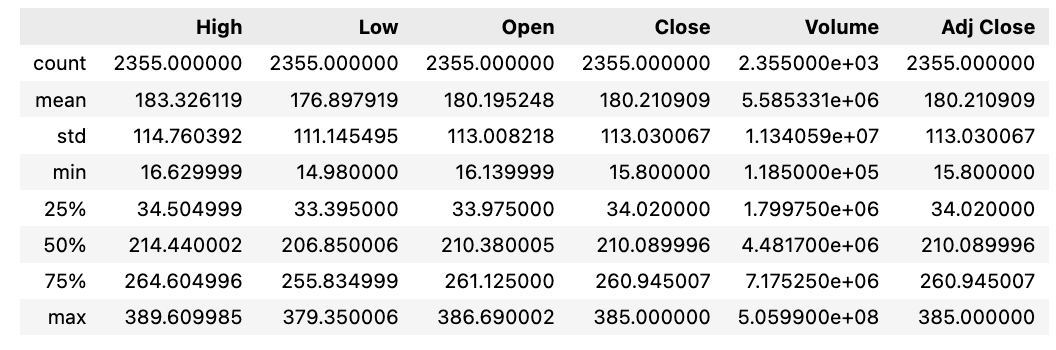
When you call upon the describe() function on a pandas DataFrame, like in the code snippet, it generates a succinct overview of statistical information pertinent to the numerical columns within the DataFrame. This summary encompasses various statistics, including the count (indicating the number of non-null entries), mean, standard deviation, minimum and maximum values, as well as percentile values such as the 25th, 50th, and 75th percentiles.
This function proves invaluable in swiftly grasping the data’s distribution and intrinsic features at a glance. It proves especially handy during the initial stages of data exploration in data science or analysis projects to swiftly gain insights into the data and pinpoint potential anomalies like outliers, absent values, or irregular characteristics.
In general, leveraging the describe() method is crucial for preliminary data investigation, synthesis, and gaining an initial understanding of the data encapsulated within a pandas DataFrame.
Verifying the presence of any absent data
Checks for missing data in tesla_df
print('No missing data') if sum(tesla_df.isna().sum()) == 0 else tesla_df.isna().sum()
This snippet of code helps to determine the presence of any missing values in the dataset called tesla_df.
It first uses the tesla_df.isna().sum() function to check how many values are missing in each column of the DataFrame. By applying sum(tesla_df.isna().sum()), the total count of missing values across the entire DataFrame is calculated.
If no missing values are found (total count of missing values equals zero), the code will display ‘No missing data’. However, if there are missing values present, it will reveal the count of missing values for each column.
Detecting and managing missing data is crucial as it can distort analyses and forecasts. Recognizing and appropriately addressing missing data is essential to ensure the accuracy and reliability of any analytical or modeling outcomes.
Creating Features
Read and analyze stock data, calculate indicators
files = os.listdir('data/raw_stocks')
stocks = {}
for file in files:
    name = file.lower().split('.')[0]
    stocks[name] = pd.read_csv('data/raw_stocks/'+file)

    stocks[name]['Return'] = round(stocks[name]['Close'] / stocks[name]['Open'] - 1, 3)
    stocks[name]['Change'] = (stocks[name].Close - stocks[name].Close.shift(1)).fillna(0)
    stocks[name]['Date'] = pd.to_datetime(stocks[name]['Date'])
    stocks[name].set_index('Date', inplace=True)
    stocks[name]['Volatility'] = stocks[name].Close.ewm(21).std()
    stocks[name]['MA7'] = ma7(stocks[name])
    stocks[name]['MA21'] = ma21(stocks[name])
    stocks[name]['Momentum'] = momentum(stocks[name].Close, 3)
    stocks[name]['RSI'] = rsi(stocks[name])
    stocks[name]['MACD'], stocks[name]['Signal'] = macd(stocks[name])
    stocks[name]['Upper_band'], stocks[name]['Lower_band'] = bollinger_bands(stocks[name])
    stocks[name].dropna(inplace=True)
    stocks[name].to_csv('data/stocks/'+name+'.csv')

stocks['tsla'].head()
Firstly, it scans the ‘data/raw_stocks’ directory to compile a list of files.
Next, it initializes an empty dictionary named ‘stocks’.
Subsequently, it executes the following steps for each file found in the directory:
- Derives the stock name by parsing the file name, converting it to lowercase, and eliminating the file extension.
- Loads the CSV file data into a Pandas DataFrame, assigning it to the respective stock’s name in the ‘stocks’ dictionary.
- Computes a range of financial metrics such as return, change, volatility, moving averages, momentum, RSI, MACD, Bollinger Bands, and then proceeds to process and store these metrics in the relevant stock’s DataFrame.
- Chooses the ‘Date’ column as the DataFrame index.
- Removes any rows that contain NaN values.
- Persists the processed data into a new CSV file in the ‘data/stocks’ directory under the relevant stock name.
Finally, it retrieves and exhibits the initial few rows of the ‘tsla’ stock data from the stored dictionary.
This code proves to be valuable for refining raw stock data, evaluating multiple technical indicators, and archiving the processed stock information into distinct CSV files for additional scrutiny, visualization, or modeling.
Our primary sources of information will be historical data and technical indicators. In addition, we intend to analyze Tesla’s news headlines to explore whether news can impact price fluctuations.
Latest Updates on Tesla in the News
We’ll be referring to the NASDAQ website as our news source. When we last checked, there were a whopping 120 pages filled with news articles spanning from January 10, 2019, to September 5, 2019.
Gets Tesla headlines from NASDAQ
headlines_list, dates_list = [], []
for i in range(1, 120):
    headlines, dates = get_tesla_headlines("https://www.nasdaq.com/symbol/tsla/news-headlines?page={}".format(i))
    headlines_list.append(headlines)
    dates_list.append(dates)
    time.sleep(1)
This script is designed to scrape headlines and dates associated with Tesla (TSLA) stock from the NASDAQ website. It achieves this by making multiple HTTP requests to various pages of the NASDAQ site through the get_tesla_headlines function, which iterates through page numbers from 1 to 119.
Each page’s headlines and dates are extracted and appended to distinct lists named headlines_list and dates_list. The script also incorporates a 1-second pause (time.sleep(1)) between requests to avoid bombarding the NASDAQ server with an excessive number of requests simultaneously. This brief interval allows the server ample time to process each request before the subsequent one is sent.
In essence, the script streamlines the process of gathering Tesla-related news headlines and publication dates from the NASDAQ site, assembling them neatly into two lists for further examination, tracking, or storage.