How To Explore Financial Time Series Data

The methods discussed in this article, however, can be applied not only to financial time series, but to many other fields as well.

In this article, you will learn how to identify outliers using rolling statistics 

— Identifying outliers using the Hampel filter

 — Identifying change points in time series

 — Detecting trends in time series

 — Utilizing the Hurst exponent to identify patterns in a time series 

— Examining common characteristics of asset returns.

Rolling statistics for detecting outliers

Observations that deviate greatly from the majority are called outliers when working with data. This can occur as a result of incorrect pricing, market events, or data processing errors. Statistical methods and machine learning algorithms can be affected heavily by outliers, leading to inaccurate or biased results. The identification and management of these outliers are therefore critical before developing any models.

Using the rolling average and standard deviation, we present a simple method that uses a filter to identify outliers. Throughout 2019 and 2020, we will examine Tesla’s stock prices.

Performing this task involves the following steps:

The following steps will help you identify outliers using rolling statistics and plot them:

The necessary libraries should be included.

import pandas as pd
import yfinance as yf

To compute Tesla’s simple returns, retrieve its stock prices for the period from 2019 to 2020.

df = yf.download("TSLA",
                 start="2019-01-01",
                 end="2020-12-31",
                 progress=False)
df["rtn"] = df["Adj Close"].pct_change()
df = df[["rtn"]].copy()

A 21-day moving window’s average and standard deviation are as follows:

df_rolling = df[["rtn"]].rolling(window=21) \
                        .agg(["mean", "std"])
df_rolling.columns = df_rolling.columns.droplevel()

Add the rolling data to the original DataFrame.

df = df.join(df_rolling)

Limits should be determined at the upper and lower ends.

N_SIGMAS = 3
df["upper"] = df["mean"] + N_SIGMAS * df["std"]
df["lower"] = df["mean"] - N_SIGMAS * df["std"]

Calculate the thresholds that will identify the outliers.

df["outlier"] = (
    (df["rtn"] > df["upper"]) | (df["rtn"] < df["lower"])
)

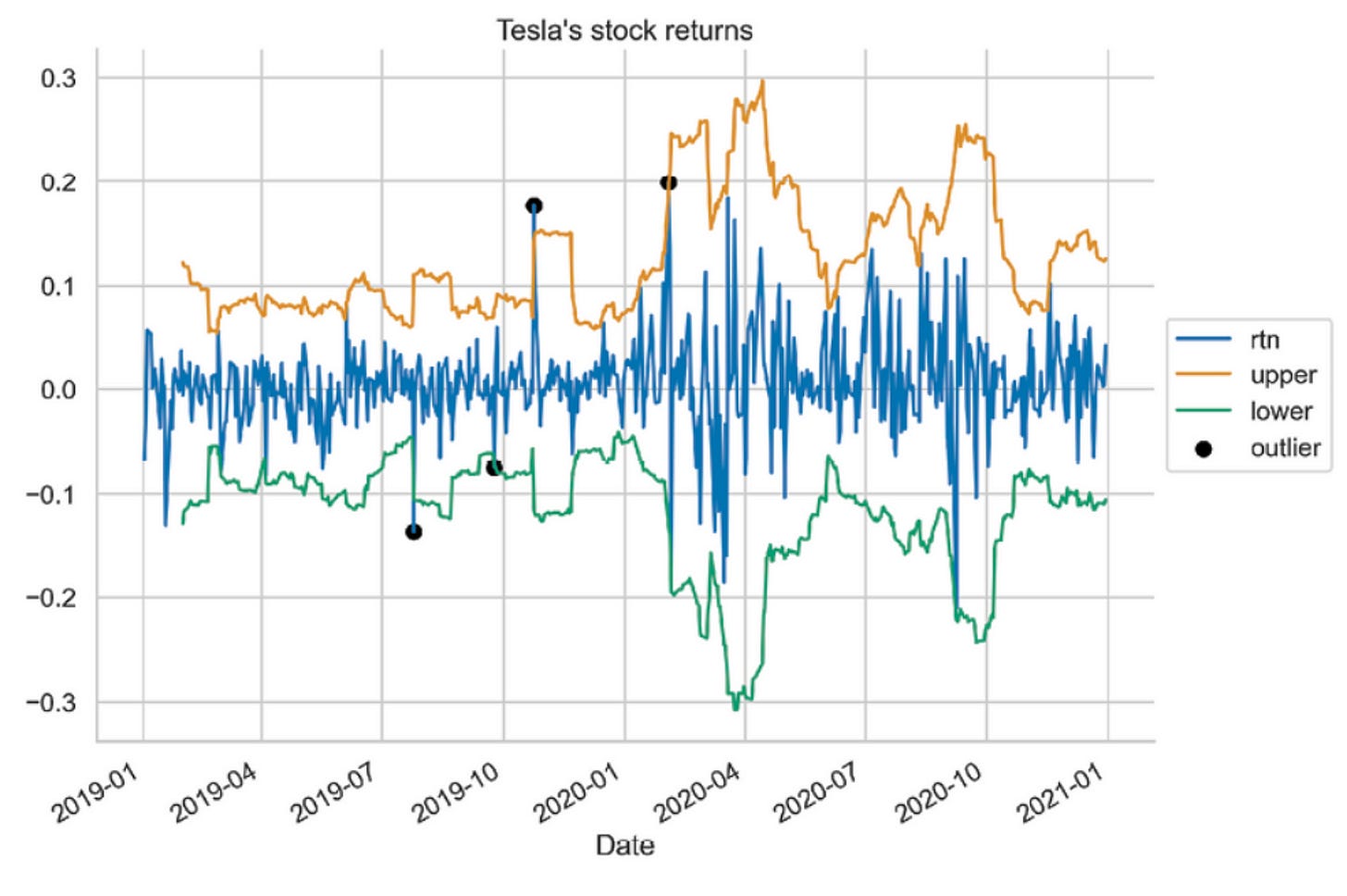
Create a plot that illustrates the returns alongside threshold values and also shows outliers.

fig, ax = plt.subplots()
df[["rtn", "upper", "lower"]].plot(ax=ax)
ax.scatter(df.loc[df["outlier"]].index,
           df.loc[df["outlier"], "rtn"],
           color="black", label="outlier")
ax.set_title("Tesla's stock returns")
ax.legend(loc="center left", bbox_to_anchor=(1, 0.5))
plt.show()

A graph is produced as a result of executing the snippet.

Data points which differ significantly from the norm are indicated by a black dot, along with the benchmarks that were used to identify them. Note that the algorithm classifies the first large return as an outlier, but the second as a normal observation when two large returns occur close together. In this case, it is possible that the first outlier affects both the rolling window and the standard deviation by influencing the moving average and standard deviation of the rolling window. As an example, look at the first quarter of 2020.

Next, we downloaded the Tesla stock price using the necessary libraries. The returns were analyzed further by selecting only the columns that contained returns. As a measure of outliers, moving statistics were calculated with a rolling window of 21 days. Considering that we are working with daily data, we selected 21 days based on the average number of trading days in a month. The reaction time can be varied by selecting alternative values. In addition, exponentially weighted moving averages may be used if that is more appropriate for your needs. The moving metrics were formulated using rolling and agg methods with a pandas DataFrame. During the statistics calculation, we removed one level of the MultiIndex to simplify the analysis.