How to Forecast Stock Prices Using Python

How to Use Differencing, Moving Averages, and ARIMA to Model Financial Data

Download entire source code at the end of article!

This project is about predicting stock prices — that means trying to guess the future price of a company’s share based on past information. A stock price is just the cost to buy one piece of a company. We try this because better guesses can help investors make smarter choices, but it’s important to know predictions are never certain.

In practice, a prediction problem means we give a model past data and ask it to forecast what comes next. That past data might be historical prices, trading volume, or simple indicators; a time series is just a list of numbers ordered by time, like daily closing prices. Preparing the right inputs matters because it guides what kind of model and tests we use later.

Real markets are noisy and change over time, so predicting them is challenging — noisy means lots of random ups and downs that aren’t useful signals. Because of that, you’ll need careful evaluation and reasonable expectations: we aim for a model that works well on new data, not one that just memorizes the past. This keeps the project grounded and useful for real decisions.

When you say “Loading and Handling Data into Pandas” for stock price prediction, think of *pandas* as the go-to toolbox for tables in Python. A *DataFrame* is just a smart table that holds your prices, dates, and any extra columns you need.

Start by loading your CSV or API data with pandas’ read_csv or read_json and tell it which column is the date. Parsing dates makes the date column a real time object, which you need for things like plotting and resampling. Set the date as the index and sort it so rows flow in time order.

Real market data often has gaps or missing values called NaN. You can drop rows, or fill them forward/backward depending on why they’re missing. Fixing gaps early prevents training a model on bad inputs and avoids errors later.

Convert data to the frequency you want, like daily or hourly, using resampling. Resampling groups times into a consistent rhythm — this helps when combining feeds or computing indicators. Also align different symbols by timestamps so features match up.

Make features like returns (percent change) and moving averages using rolling windows — a rolling window is a short time slice you slide along to summarize recent behavior. Finally, split by date into training and test sets without shuffling to avoid leaking future info into the past. This keeps evaluation honest.

import pandas as pd
import numpy as np
import matplotlib.pylab as plt
%matplotlib inline
from matplotlib.pylab import rcParams
rcParams[’figure.figsize’] = 15, 6

Think of these lines as bringing the tools to your workbench so you can prepare, calculate, and paint the story of stock prices. The first line pulls in pandas and gives it the nickname pd so you can work with tables and time series easily; pandas is like a spreadsheet inside Python that makes dates and columns simple to manipulate. Next we import numpy as np, which is the fast number-crunching toolbox — numpy is a library for numerical arrays and math that underpins many calculations. Then we import matplotlib.pylab as plt so we have a painter’s palette for charts; matplotlib is the plotting library that turns numbers into visible trends. The %matplotlib inline instruction is an IPython magic that tells a Jupyter notebook to display plots right below your code cell so you can see the visuals immediately; this is notebook-specific rather than a general Python statement. Finally, we bring in rcParams from matplotlib.pylab and set rcParams[‘figure.figsize’] = 15, 6 to change the default canvas size to a wide, short rectangle — rcParams is a dictionary of plotting defaults that controls how plots look without repeating size settings every time.

Together these lines set up data structures, fast math, and plotting defaults so you can load historical prices, compute indicators, and visualize predictions versus reality as you build your stock price prediction project.

data = pd.read_csv(’/home/sash/Documents/Sem_6/SMAI/Major_Project/Final-Data/FB.csv’)
print data.head()
print ‘\n Data Types:’
print data.dtypes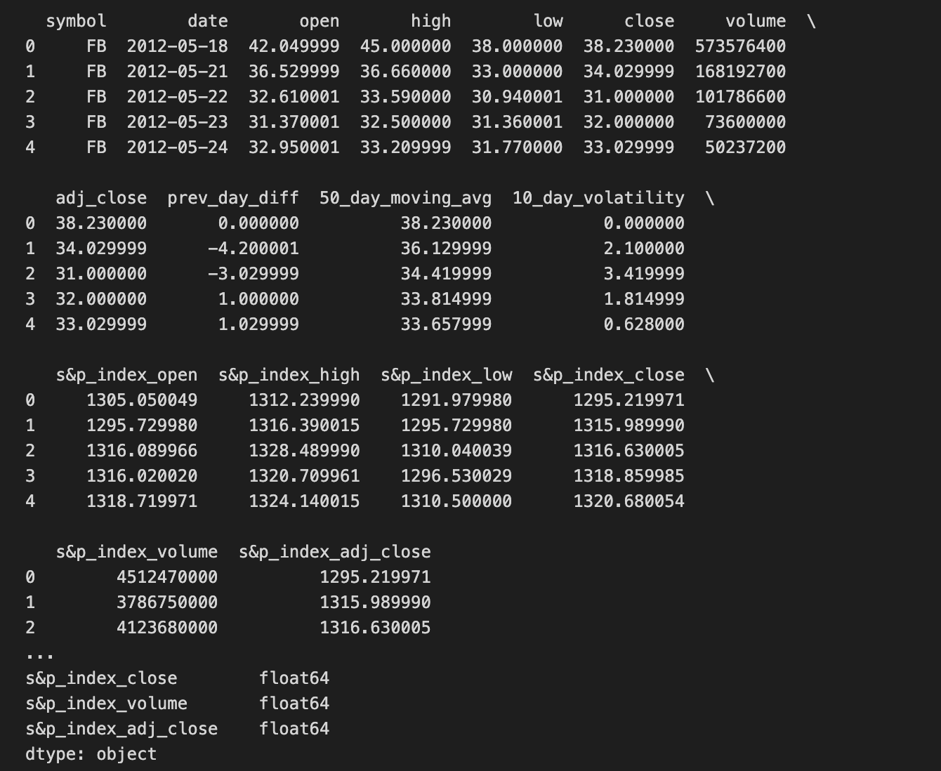

We’re trying to bring into Python a table of historical Facebook prices so we can examine and eventually feed it to a prediction model. The first line asks pandas (pd is the common nickname for the pandas library) to read a CSV file at the given path and load it into a DataFrame, which is pandas’ two-dimensional table-like object for holding rows and columns — think of a DataFrame as a spreadsheet you can manipulate in code. Reading the file is like opening the ledger where each row is a daily record and each column is a field such as date, open, close, volume.

Next, print data.head() flips the ledger to the front and shows the first few entries so you can quickly eyeball whether the import worked and what columns look like; by default it shows the first five rows. The explicit print of ‘\n Data Types:’ simply writes a label to separate sections of output for clarity. Finally, print data.dtypes lists the data type of each column (integer, float, object/text, etc.), which is crucial because the kind of model you build depends on having numbers where numbers belong and dates parsed correctly — data types determine how you can compute and compare values. Together these steps are basic but essential preparation: you load the historical data, inspect a sample, and verify the types before you clean, engineer features, and train your stock price prediction model.

Read your date column as a *datetime* format. A datetime is just a date and time value that your code can understand as a timeline instead of plain text, so your program knows January 1 comes before February 1.

This matters for stock price prediction because you’ll sort, slice by range, resample (like turning minute data into daily data), and compute rolling averages. If dates stay as text, those time-based operations won’t work right and results can be wrong.

When loading data, tell your tool to parse dates (for example, many libraries have a “parse dates” option) or convert the column afterward with a date-conversion function. After that, set the datetime column as the table’s index (the row labels) so it’s easy to pick ranges like “last month” or “last year.”

dateparse = lambda dates: pd.datetime.strptime(dates, ‘%Y-%m-%d’)
# dateparse(’1962-01’)
data = pd.read_csv(’/home/sash/Documents/Sem_6/SMAI/Major_Project/Final-Data/FB.csv’, parse_dates=’date’, \
                   index_col=’date’,date_parser=dateparse)
print data.head()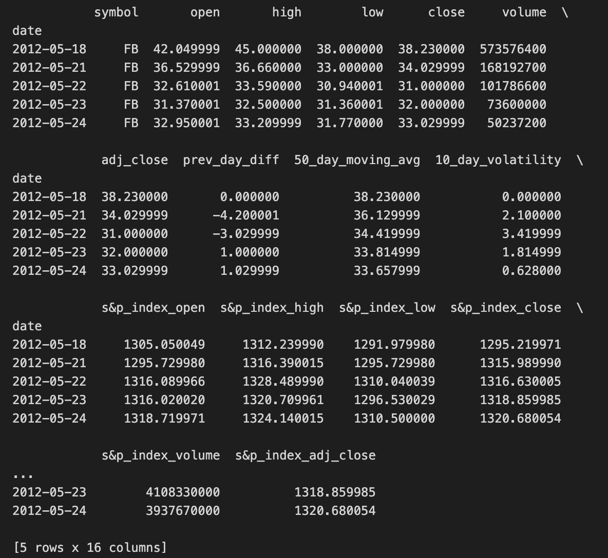

We want to load Facebook stock data and make the dates useful for time-series work, so the first line defines a small reusable recipe card that converts a date string into a Python datetime object: dateparse = lambda dates: pd.datetime.strptime(dates, ‘%Y-%m-%d’). A lambda is a compact way to make a tiny function in place, and here it wraps strptime so each date string like “2020–01–15” becomes a proper datetime the computer can understand.

The commented line shows someone experimenting with that parser: # dateparse(‘1962–01’) — it’s an example call, though the format should match ‘%Y-%m-%d’ or it will complain. Next, we open the CSV file with pandas.read_csv and give a few instructions: parse_dates=’date’ tells pandas to convert the column named “date” into actual date objects, index_col=’date’ makes those dates the row labels so you can slice by time, and date_parser=dateparse supplies our custom recipe card to do the conversion. Key concept: a datetime index lets you treat rows by time (slice ranges, resample, align series), which is essential for any temporal model.

Finally, print data.head() shows the first few rows so you can check that dates parsed correctly and the price columns look sane. With a clean, date-indexed table, you’re ready to compute returns, engineer features, and feed time-aware models for stock price prediction.

#check datatype of index
data.index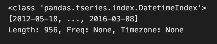

We start with a little note written for the reader: “#check datatype of index” — that’s a human instruction, like putting a sticky note on a recipe card to remind you what to verify before you cook. The next line, data.index, is our actual peek: in an interactive Python session or notebook, simply evaluating data.index returns the Index object that labels each row of the table. The index is the set of labels that identify each row in a DataFrame; it’s the backbone for alignment and time-based operations. By looking at data.index you learn whether those labels are plain integers, strings, or a specialized DatetimeIndex that understands dates and times.

Knowing the index type is important because if your labels are timestamps you gain access to convenient time-series tools (resampling, rolling windows, slicing by date); if they are just strings you may need to convert them. Think of it like checking whether your ingredients are fresh fruit or canned fruit before following a recipe — the rest of the steps change depending on that fact. In the stock price prediction project, confirming the index is a DatetimeIndex lets you reliably build time-based features and align prices by trading days, which keeps your forecasts honest and well-timed.

#convert to time series:
ts = data[’adj_close’]
ts.head(10)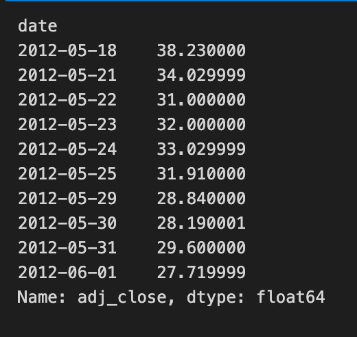

We’re taking a single column of market data and turning it into the time-ordered series that our forecasting recipes will use. The line that assigns ts = data[‘adj_close’] is like reaching into a pantry and pulling out the one ingredient we care about — the adjusted closing price — from a larger grocery cart of columns. In pandas, selecting a column returns a Series — a one-dimensional labeled array. That Series holds the price values in the original row order and will be the sequence our models read as “values over time.”

The call ts.head(10) is a gentle taste test: it prints the first ten entries so you can quickly check that the values look right and that the ordering matches dates you expect. head() does not change the Series; it’s a non-destructive peek. Using adjusted close specifically is important because it accounts for dividends and splits, giving a cleaner view of true investor return.

After this, you typically ensure the DataFrame or Series has a datetime index and then visualize, difference, or normalize it before feeding into models. In short, we’ve isolated and inspected the single time series that will become the core input for our stock price prediction pipeline.

A TS array is just a time-ordered list of numbers, like daily stock prices lined up by date. Thinking of it that way helps: the order matters because earlier values can influence later ones, which is exactly what prediction models use.

You can pick values by position using integer indexing or slices, for example the first 100 days or the last 30 days. This is handy for making training and test sets because you usually keep time order intact — you don’t want future data mixed into the past.

You can also index by dates when your array has timestamps, so you ask for “prices from Jan–Mar 2020” directly. That makes it easy to align different series (like prices and volumes) by calendar dates so every row really corresponds to the same day.

Boolean masks let you select days that meet a condition, like days with volume above a threshold. This is useful for filtering out noisy or irrelevant days before making features.

For models you often build sliding windows: take the last N days as input and the next day as the label. Doing this consistently avoids *lookahead bias*, which is when the model accidentally sees future information. Aligning, slicing, and careful handling of missing values are small steps that prevent big mistakes later.

#1. Specific the index as a string constant:
ts[’2012-05-18’]

Think of the program as asking the time-stamped ledger for a single day’s entry so you can inspect or use that price in your prediction work. The comment is a simple note of intent: we want to specify the index using a string constant, i.e., name the exact date we care about. The next line ts[‘2012–05–18’] is like telling a librarian “please hand me the May 18, 2012 page” — it asks the time series object ts for the record labeled with that date.

If ts is a pandas Series or DataFrame with a DatetimeIndex, pandas will parse the string and return the row or value for that label. Key concept: label-based indexing means you ask for data by its label (the date) rather than by numeric position. If there is exactly one entry for that day you get a single price (a scalar); if there are multiple intraday rows for the same date you receive a smaller time series for that day. Using a string date is a quick, readable way to pull out a specific observation without counting positions, and for explicitness you could also write ts.loc[‘2012–05–18’].

Grabbing a single day’s price this way is a small but important step when building a stock price prediction pipeline: you use precise historical values to compute returns, validate predictions, or create training targets.