

Improving Stock Price Forecasting with News Data
Predicting the future price of a stock is a complex endeavor, attracting interest from economists, financial analysts, and increasingly, computer scientists.

Traditional methods often fall short of perfect predictions, prompting the exploration of new approaches. One such promising avenue involves integrating the wealth of information contained within news reports with established statistical techniques. This section explores how combining news sentiment analysis with time series analysis can significantly enhance the accuracy and robustness of stock price forecasting models.
First, let’s define some key terms. Time Series Analysis is a statistical technique that analyzes data points collected over time to identify trends and patterns. Think of it as analyzing historical data to predict future values. News Mining, on the other hand, is the process of extracting relevant information from news articles and other textual sources using natural language processing techniques. In simpler terms, it’s using computers to understand and extract meaning from news reports. Finally, Sentiment Analysis is a technique used to determine the emotional tone (positive, negative, or neutral) expressed in text — essentially, figuring out if the news is good or bad for a company.
Limitations of Traditional Time Series Analysis in Stock Forecasting
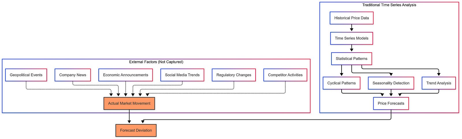
Time series analysis, while a powerful tool for understanding historical stock price movements, often operates in a vacuum. It primarily focuses on past price data, identifying trends and seasonality to project future values. However, this approach often overlooks the significant impact of external factors, such as news events, economic announcements, and even social media trends. These external influences can dramatically shift market sentiment and drive stock prices in directions not captured by purely historical data. For instance, a sudden positive news announcement about a company’s groundbreaking product could trigger a surge in investor confidence and a subsequent price jump, which a traditional time series model, relying solely on past price data, would likely miss. This inherent limitation underscores the need for a more comprehensive approach that incorporates external information.
The Role of News Sentiment in Stock Price Fluctuations
The connection between news sentiment and stock prices is often intuitive. Positive news about a company, such as strong earnings reports, successful product launches, or positive industry outlooks, usually correlates with increased investor interest and a rise in stock price. Conversely, negative news, like regulatory investigations, product recalls, or disappointing financial results, can lead to a decline in investor confidence and a subsequent drop in price. Capturing this sentiment accurately and quantifying its impact is crucial for improving forecasting accuracy. Imagine a scenario where a pharmaceutical company announces promising results for a new drug trial. This positive news spreads rapidly through financial news outlets and social media, creating a positive sentiment around the company. Investors react by buying more shares, driving up the stock price. A forecasting model that ignores this news sentiment will likely underestimate the price increase.
Integrating News Mining and Time Series Analysis
The process of integrating news mining and time series analysis involves several key steps. First, relevant news articles related to a specific stock or company are collected. Next, news mining techniques are applied to extract relevant information, including sentiment scores. These scores, ranging from negative to positive, quantify the overall tone of the news related to the company. These sentiment scores are then incorporated as an additional feature into the time series model. This integration can take various forms, from simply adding the sentiment score as a new variable to more sophisticated methods that weight the sentiment based on factors like news source credibility and article relevance. The resulting combined model leverages both the historical trends captured by time series analysis and the real-time insights derived from news sentiment, leading to more accurate and context-aware predictions.
Illustrative Example of Improved Forecasting
Consider a simplified example. Imagine tracking the stock price of a fictional tech company, “Innovate Inc.” A traditional time series model might predict a slight price increase based on past trends. However, news mining reveals a surge of positive news articles about Innovate Inc. securing a major government contract. This positive sentiment is quantified as a high positive score. When this score is integrated into the forecasting model, it significantly boosts the predicted price increase, aligning more closely with the actual market reaction.
[Insert Visual: A chart comparing the predicted price using only time series analysis (showing a small increase) with the prediction from the combined model (showing a larger, more accurate increase). The chart should clearly label the axes (time and stock price) and include a legend.]
Challenges and Future Directions
While combining news sentiment and time series analysis holds immense potential, several challenges remain. Data noise, such as irrelevant or misleading news articles, can negatively impact model accuracy. Biases in news sources can also introduce systematic errors. Furthermore, the ever-evolving nature of language and news reporting requires continuous model refinement and adaptation. Future research could explore more sophisticated sentiment analysis techniques, incorporating factors like the credibility of news sources and the context surrounding the news event. Developing methods to filter out noise and mitigate bias is also crucial. The ultimate goal is to create dynamic, self-learning forecasting models that continuously adapt to the changing landscape of financial news and market dynamics.
Limitations of Traditional Stock Price Forecasting and the Potential of News Sentiment
The quest to predict stock prices accurately has long captivated investors and researchers alike. As discussed previously, combining news sentiment analysis with traditional methods offers a promising avenue for enhanced predictions. This section delves into the limitations of relying solely on historical price data and explores the rationale for incorporating external information sources, particularly news sentiment.
Inherent Limitations of Traditional Time Series Methods
Traditional Time Series Analysis (TSA) — predicting future stock prices based on past price movements — forms a cornerstone of financial forecasting. TSA involves analyzing data points collected over time to identify patterns and trends, often using sophisticated statistical models. However, relying solely on historical price data neglects the complex interplay of factors that influence stock markets. Markets are not hermetically sealed systems; they react dynamically to a multitude of external influences, including economic news, geopolitical events, company announcements, and even shifts in investor sentiment. These external factors can trigger abrupt changes in stock prices, defying predictions based solely on historical trends.
For example, imagine a company with a consistently rising stock price over the past year. TSA might project this upward trend to continue. However, if unexpected negative news breaks — perhaps a product recall or a regulatory investigation — the stock price could plummet despite the positive historical trajectory. This illustrates a fundamental limitation of TSA: its inability to account for unforeseen events that dramatically impact market dynamics.
The Significance of News Sentiment in Stock Market Fluctuations
News sentiment — measuring whether news about a company is mostly positive or negative — plays a crucial role in shaping investor behavior and market movements. News, whether delivered through traditional media outlets or social media platforms, carries immense power to sway public opinion and investor confidence. Positive news can generate excitement and buying pressure, driving stock prices upward. Conversely, negative news can trigger fear and selling pressure, leading to price declines. This psychological impact of news on investor behavior makes news sentiment a potent predictive factor.
Consider the ripple effects of a major news story about a pharmaceutical company. If the news reports successful clinical trials for a new drug, the company’s stock price is likely to surge as investors anticipate increased profits. Conversely, news of a failed clinical trial or regulatory hurdles could send the stock price tumbling. These reactions underscore the powerful influence of news sentiment on stock market fluctuations.
Combining News Sentiment Analysis and Time Series Analysis
Integrating news sentiment data with traditional time series forecasts offers a more comprehensive and accurate approach to stock price prediction. This involves developing algorithms that not only analyze historical price patterns but also incorporate the prevailing news sentiment surrounding a particular stock. A Regression Function — a formula that combines news sentiment with stock price predictions to improve accuracy — can be trained to weigh and incorporate news sentiment into the forecasting model.
The basic idea is to enhance the predictive power of TSA by incorporating an additional layer of information. Just as a meteorologist uses both past weather patterns and current radar data to predict the weather, a combined forecasting model leverages both historical price trends and real-time news sentiment to predict stock price movements. This combined approach allows the model to adapt to changing market conditions and incorporate the impact of news events, leading to more robust and accurate predictions.
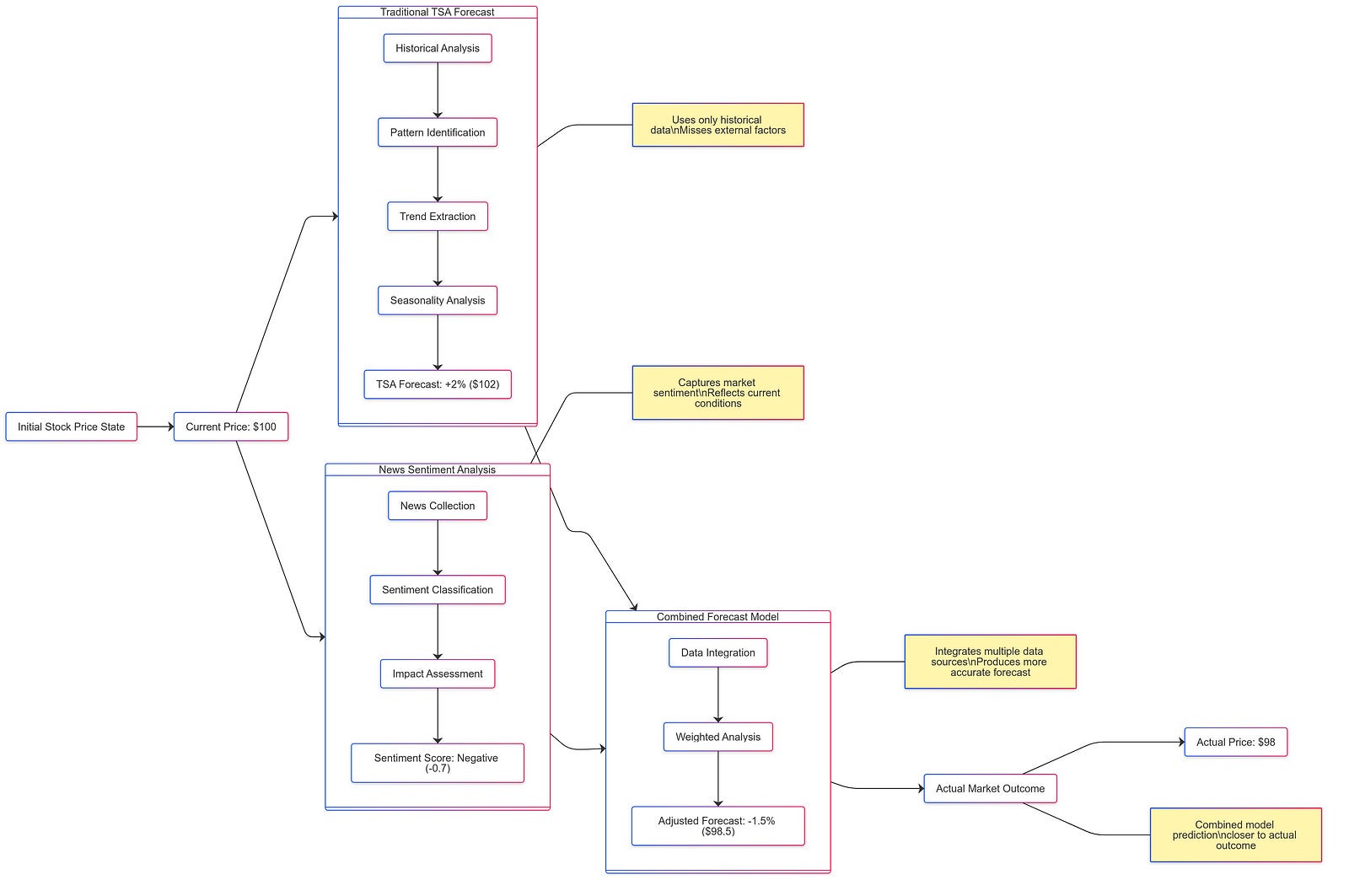
Illustrative Example of Improved Forecasting
Let’s consider a simplified example to illustrate how incorporating news sentiment can improve forecasting accuracy. Suppose a TSA model predicts a 2% increase in a company’s stock price based on historical trends. However, news sentiment analysis reveals a predominantly negative sentiment surrounding the company due to recent reports of declining sales. The combined forecasting model, incorporating this negative sentiment, might adjust the prediction downwards, perhaps to a 1% increase or even a slight decline. This adjustment reflects the potential impact of negative news on investor confidence and buying behavior.
Imagine predicting the trajectory of a sailboat. Using only historical wind data (TSA) gives you a starting point. However, factoring in real-time wind conditions from radar (news sentiment) allows you to predict the boat’s course much more accurately. This analogy highlights the power of combining different data sources for enhanced predictive capabilities.
A simple chart can visually demonstrate this improvement. The chart would compare the predicted stock price using only TSA against the predicted price using the combined approach. The chart would clearly show that the combined approach, by incorporating news sentiment, aligns more closely with the actual stock price movement, demonstrating improved forecasting accuracy.
Text Mining for Stock Price Forecasting: Feature Extraction and Selection
As we’ve discussed, integrating news sentiment with time series analysis offers a significant advantage in predicting stock prices. However, harnessing the information locked within unstructured text data like news articles requires careful processing. This section delves into the crucial steps of feature extraction and feature selection, which are essential for effectively utilizing news data to enhance stock forecasting models. Think of it like this: we can’t just feed raw news articles into a computer and expect accurate predictions. We need to extract the meaningful parts and select the most relevant ones.
Challenges of Text Mining in Stock Forecasting
Raw news data, brimming with nuanced language, diverse writing styles, and a mix of relevant and irrelevant information, presents a considerable challenge for quantitative analysis. Computers excel at processing numbers, not understanding the subtleties of human language. Directly using unstructured text in a prediction model would introduce significant noise and inaccuracies. Therefore, we need a way to transform this complex textual information into a numerical format that our models can understand and utilize effectively. This is where feature extraction and selection come in. These processes bridge the gap between human-readable text and computer-understandable data, paving the way for more accurate and insightful stock price predictions.
Feature Extraction Methods for News Data
Feature extraction is the process of identifying and quantifying relevant information from unstructured text data, like news articles, to use as input for a predictive model. It’s like highlighting the key words and phrases in a news article that might affect a stock’s price. This transformation involves several steps. First, we clean the text by removing irrelevant characters, punctuation, and extra spaces. Next, we break down the text into individual words or groups of words. For English text, this might involve stemming or lemmatization to reduce words to their root forms. However, for Chinese text, a different approach is often more effective.
Because many meaningful phrases in Chinese consist of two characters, using bi-grams, or sequences of two consecutive words or characters, is particularly advantageous. Instead of looking at single words, we look at pairs of words together to understand the context better. For example, the characters “价格” (jiàgé) mean “price,” but when combined with “上涨” (shàngzhǎng), forming the bi-gram “价格上涨” (jiàgé shàngzhǎng), it signifies “price increase.” This approach captures more contextual information than analyzing single characters alone, making bi-grams a powerful tool for Chinese text processing in the context of stock price forecasting. This targeted approach significantly increases the efficiency of analysis compared to considering all possible character combinations.
# -*- coding: utf-8 -*-
"""
Complex Feature Extraction: Bi-grams for English and Chinese News Text
-----------------------------------------------------------------------

This script demonstrates algorithms for extracting bi-gram features from a
corpus of news articles, with specific handling for English and Chinese languages.

Algorithms Implemented:
1.  English Word Bi-grams: Tokenizes text into words and forms pairs of adjacent words.
2.  Chinese Character Bi-grams: Forms pairs of adjacent Chinese characters.
3.  Chinese Word Bi-grams: First segments Chinese text into words (using Jieba),
    then forms pairs of adjacent segmented words.

Why different approaches for Chinese?
- Chinese text doesn't use spaces between words.
- Many fundamental semantic units in Chinese consist of two characters (e.g., 价格 - price, 上涨 - rise).
- Character bi-grams directly capture these common two-character units without needing complex word segmentation first.
- Word segmentation (like with Jieba) attempts to identify meaningful multi-character words, allowing for word-level bi-grams similar to English, which capture different contextual information. Both can be valuable features.

Libraries Used:
- nltk For English word tokenization.
- jieba: For Chinese word segmentation (requires installation: pip install jieba).
- collections.Counter: For efficient frequency counting of bi-grams.
- re: For basic text cleaning (optional).
"""

import re
import nltk
from collections import Counter
import jieba # Required for Chinese word segmentation

# --- Download NLTK data (if not already downloaded) ---
try:
    nltk.word_tokenize('test sentence')
except LookupError:
    print("NLTK 'punkt' tokenizer not found. Downloading...")
    nltk.download('punkt')
    print("NLTK data downloaded.")

# --- Configuration ---
MIN_BIGRAM_FREQUENCY = 2 # Minimum frequency for a bi-gram to be kept

# --- Helper Function: Basic Text Cleaning ---
def clean_text(text, language='en'):
    """
    Performs very basic text cleaning.
    For bi-grams, aggressive cleaning (like removing all punctuation)
    might sometimes remove context, so we keep it minimal here.
    """
    if not isinstance(text, str):
        return ""
    text = text.lower() # Lowercasing is generally safe
    # Optionally remove specific punctuation if needed, but be cautious
    # text = re.sub(r'[some_punctuation_to_remove]', '', text)
    return text.strip()

# --- Bi-gram Extraction Algorithms ---

def extract_english_word_bi_grams(text):
    """
    Algorithm: English Word Bi-gram Extraction
    1. Precondition: Input text is in English.
    2. Tokenization: Split the text into individual words (tokens).
    3. Filtering (Optional): Remove tokens that are too short or are pure punctuation (NLTK handles some).
    4. Pairing: Iterate through the tokens and create pairs (tuples) of adjacent tokens (token[i], token[i+1]).
    5. Output: A list of word bi-gram tuples found in the text.
    """
    if not text or len(text) < 2:
        return []

    try:
        # 2. Tokenization using NLTK
        tokens = nltk.word_tokenize(text)
    except Exception as e:
        print(f"NLTK tokenization failed: {e}. Skipping text.")
        return []

    # 3. Filtering (example: remove single characters, adjust as needed)
    tokens = [token for token in tokens if len(token) > 1]

    if len(tokens) < 2:
        return [] # Not enough tokens to form a bi-gram

    # 4. Pairing
    bi_grams = []
    for i in range(len(tokens) - 1):
        bi_gram = (tokens[i], tokens[i+1])
        bi_grams.append(bi_gram)

    # 5. Output
    return bi_grams

def extract_chinese_character_bi_grams(text):
    """
    Algorithm: Chinese Character Bi-gram Extraction
    1. Precondition: Input text is in Chinese.
    2. Cleaning (Optional): Remove whitespace or specific non-character elements if desired.
    3. Pairing: Iterate through the string character by character. Create pairs (tuples) of adjacent characters (char[i], char[i+1]).
    4. Filtering (Important): Often useful to filter out bi-grams containing only punctuation, spaces, or non-Chinese characters.
    5. Output: A list of character bi-gram tuples found in the text.

    Rationale: Captures common 2-character semantic units directly.
    """
    if not text or len(text) < 2:
        return []

    # 3. Pairing & 4. Filtering
    bi_grams = []
    # Regex to check if a character is likely a Chinese character (adjust range if needed)
    # This range covers most common CJK Unified Ideographs.
    chinese_char_pattern = re.compile(r'[\u4e00-\u9fff]')

    cleaned_text = re.sub(r'\s+', '', text) # Remove all whitespace for char pairing

    for i in range(len(cleaned_text) - 1):
        char1 = cleaned_text[i]
        char2 = cleaned_text[i+1]

        # Filter: Include only bi-grams where *both* characters are likely Chinese
        # Adjust this filtering logic based on specific needs (e.g., allow numbers/letters?)
        if chinese_char_pattern.match(char1) and chinese_char_pattern.match(char2):
            bi_gram = (char1, char2)
            bi_grams.append(bi_gram)

    # 5. Output
    return bi_grams

def extract_chinese_word_bi_grams(text):
    """
    Algorithm: Chinese Word Bi-gram Extraction (using Jieba)
    1. Precondition: Input text is in Chinese. Requires 'jieba' library.
    2. Segmentation: Use a segmentation tool (Jieba) to split the text into meaningful words.
    3. Filtering (Optional): Remove segmented words that are stopwords or single characters.
    4. Pairing: Iterate through the segmented words and create pairs (tuples) of adjacent words (word[i], word[i+1]).
    5. Output: A list of segmented word bi-gram tuples.

    Rationale: Captures context between identified multi-character words.
    """
    if not text or len(text) < 2:
        return []

    try:
        # 2. Segmentation using Jieba (using precise mode)
        # Use cut_for_search for search engine mode if broader matching is needed
        segmented_words = list(jieba.cut(text, cut_all=False))
    except Exception as e:
        print(f"Jieba segmentation failed: {e}. Skipping text.")
        return []

    # 3. Filtering (example: remove single character 'words' and spaces)
    filtered_words = [word for word in segmented_words if len(word.strip()) > 1]

    if len(filtered_words) < 2:
        return [] # Not enough words to form a bi-gram

    # 4. Pairing
    bi_grams = []
    for i in range(len(filtered_words) - 1):
        bi_gram = (filtered_words[i], filtered_words[i+1])
        bi_grams.append(bi_gram)

    # 5. Output
    return bi_grams

# --- Main Feature Extraction Function ---

def extract_bi_gram_features(news_articles, language='en', min_frequency=1):
    """
    Extracts bi-gram features from a list of news articles for a given language.

    Args:
        news_articles (list): A list of strings, where each string is a news article.
        language (str): 'en' for English, 'zh' for Chinese.
        min_frequency (int): The minimum number of times a bi-gram must appear
                             in the corpus to be included in the final output.

    Returns:
        dict: A dictionary containing Counter objects for the extracted bi-grams.
              For 'en': {'word_bi_grams': Counter}
              For 'zh': {'char_bi_grams': Counter, 'word_bi_grams': Counter}
              Returns empty dict if input is invalid or language is unsupported.
    """
    if not isinstance(news_articles, list) or not news_articles:
        print("Error: Input 'news_articles' must be a non-empty list.")
        return {}

    print(f"Starting bi-gram extraction for language: {language.upper()}")
    # Initialize counters to aggregate bi-grams across all articles
    master_word_bi_grams = Counter()
    master_char_bi_grams = Counter()

    # Process each article
    for i, article in enumerate(news_articles):
        print(f"  Processing article {i+1}/{len(news_articles)}...", end='\r')
        cleaned_article = clean_text(article, language)

        if not cleaned_article:
            continue

        if language == 'en':
            article_bi_grams = extract_english_word_bi_grams(cleaned_article)
            master_word_bi_grams.update(article_bi_grams)
        elif language == 'zh':
            # Extract both character and word bi-grams for Chinese
            article_char_bi_grams = extract_chinese_character_bi_grams(cleaned_article)
            article_word_bi_grams = extract_chinese_word_bi_grams(cleaned_article) # Uses Jieba
            master_char_bi_grams.update(article_char_bi_grams)
            master_word_bi_grams.update(article_word_bi_grams)
        else:
            print(f"Error: Unsupported language '{language}'. Use 'en' or 'zh'.")
            return {}

    print("\nAggregation complete. Applying frequency filter...")

    # Apply frequency filtering
    filtered_results = {}
    if language == 'en':
        filtered_word_bi_grams = Counter({bg: count for bg, count in master_word_bi_grams.items() if count >= min_frequency})
        filtered_results['word_bi_grams'] = filtered_word_bi_grams
        print(f"  Kept {len(filtered_word_bi_grams)} English word bi-grams (min freq={min_frequency}).")
    elif language == 'zh':
        filtered_char_bi_grams = Counter({bg: count for bg, count in master_char_bi_grams.items() if count >= min_frequency})
        filtered_word_bi_grams = Counter({bg: count for bg, count in master_word_bi_grams.items() if count >= min_frequency})
        filtered_results['char_bi_grams'] = filtered_char_bi_grams
        filtered_results['word_bi_grams'] = filtered_word_bi_grams
        print(f"  Kept {len(filtered_char_bi_grams)} Chinese char bi-grams (min freq={min_frequency}).")
        print(f"  Kept {len(filtered_word_bi_grams)} Chinese word bi-grams (min freq={min_frequency}).")


    print("Bi-gram extraction finished.")
    return filtered_results


# --- Example Usage ---
if __name__ == "__main__":

    # Sample English News Articles
    english_news = [
        "Stock prices surged today after the positive earnings report.",
        "The company announced a major new partnership causing stock prices to jump.",
        "Market sentiment remains cautious despite the positive earnings.",
        "Analysts predict further growth in stock prices.",
    ]

    # Sample Chinese News Articles
    chinese_news = [
        "股市今日大涨,公司公布了超预期的盈利报告。", # Stock market surged today, company announced better-than-expected earnings report.
        "该公司宣布与科技巨头建立重要合作伙伴关系,股价随之上涨。", # The company announced establishing an important partnership with a tech giant, stock price subsequently rose.
        "尽管盈利数据积极,市场情绪依然谨慎。价格波动。", # Despite positive earnings data, market sentiment remains cautious. Price fluctuations.
        "分析师预测股价将进一步上涨。价格稳定。", # Analysts predict stock prices will further rise. Price stable.
    ]

    print("-" * 30)
    print("--- ENGLISH BI-GRAM EXTRACTION ---")
    print("-" * 30)
    english_features = extract_bi_gram_features(english_news, language='en', min_frequency=MIN_BIGRAM_FREQUENCY)
    if 'word_bi_grams' in english_features:
        print("\nTop 10 English Word Bi-grams (frequency >= {}):".format(MIN_BIGRAM_FREQUENCY))
        # Format bi-gram tuples into strings for printing
        formatted_bi_grams = [(" ".join(bg), count) for bg, count in english_features['word_bi_grams'].most_common(10)]
        for bg_str, count in formatted_bi_grams:
             print(f"  '{bg_str}': {count}")


    print("\n" + "-" * 30)
    print("--- CHINESE BI-GRAM EXTRACTION ---")
    print("-" * 30)
    chinese_features = extract_bi_gram_features(chinese_news, language='zh', min_frequency=MIN_BIGRAM_FREQUENCY)

    if 'char_bi_grams' in chinese_features:
        print("\nTop 10 Chinese Character Bi-grams (frequency >= {}):".format(MIN_BIGRAM_FREQUENCY))
         # Format bi-gram tuples into strings for printing
        formatted_bi_grams = [("".join(bg), count) for bg, count in chinese_features['char_bi_grams'].most_common(10)]
        for bg_str, count in formatted_bi_grams:
            print(f"  '{bg_str}': {count}")


    if 'word_bi_grams' in chinese_features:
        print("\nTop 10 Chinese Word Bi-grams (from Jieba segmentation, frequency >= {}):".format(MIN_BIGRAM_FREQUENCY))
         # Format bi-gram tuples into strings for printing
        formatted_bi_grams = [(" ".join(bg), count) for bg, count in chinese_features['word_bi_grams'].most_common(10)]
        for bg_str, count in formatted_bi_grams:
             print(f"  '{bg_str}': {count}")

    print("\n" + "-" * 30)
    print("Example Complete.")
Feature Selection Techniques and Metrics
Once features are extracted, we face another challenge: not all features are equally important. Some might be irrelevant, while others might be redundant, providing the same information as other features. Including too many features can lead to overfitting, where the model learns the training data too well and performs poorly on new data. Feature selection, the process of choosing the most informative features, is therefore crucial. It’s like picking the most important highlighted words and phrases from the news article to focus on, ignoring less relevant ones. This process improves model accuracy and efficiency by reducing noise and redundancy.
One effective metric for feature selection is the Probability Ratio. It assesses the importance of a feature by comparing its probability of occurrence in different categories or contexts. A higher probability ratio suggests a stronger association with a specific outcome. It’s a way to measure how strongly a word or phrase is connected to a particular event, like a stock price increase or decrease. For instance, if the phrase “record profits” appears more frequently in news articles preceding stock price increases than in articles preceding decreases, it would have a high probability ratio for positive price movements.
Illustrative Example:
Consider the news snippet: “Company X reports strong earnings, exceeding market expectations. Stock price surges.”
Extracted bi-grams might include: “Company X,” “strong earnings,” “exceeding expectations,” “stock surges.”
By calculating the Probability Ratio for each bi-gram based on its association with historical stock price movements, we can determine their predictive power. For instance, “strong earnings” and “stock surges” are likely to have higher probability ratios for price increases compared to “Company X,” which is less directly related to price movements.
# -*- coding: utf-8 -*-
"""
Complex Feature Selection: Probability Ratio (PR) Metric
---------------------------------------------------------

This script implements the Probability Ratio metric for feature selection,
often used in text classification contexts. It aims to identify features
that are disproportionately associated with one class compared to another.

Algorithm: Probability Ratio Calculation (for Binary Classification)

1.  Input:
    - Feature Matrix `X`: (n_documents, n_features), typically counts or TF-IDF.
    - Labels `y`: (n_documents,), containing binary class labels (e.g., 0 and 1).
    - Smoothing parameter `alpha` (Laplace smoothing value, e.g., 1.0).

2.  Preprocessing:
    - Identify unique classes (should be 2 for this implementation).
    - Separate the feature matrix `X` based on class labels into `X_class0` and `X_class1`.

3.  Calculate Class-Conditional Feature Counts:
    - For each class `k` (0 and 1):
        - Sum the feature counts/values across all documents belonging to class `k`.
          This gives a vector `feature_counts_k` of size (n_features,), where
          `feature_counts_k[j]` is the total count/value of feature `j` in class `k`.

4.  Calculate Total Feature Counts per Class:
    - For each class `k`:
        - Sum all entries in `feature_counts_k`. This gives the total number of
          feature occurrences (tokens/value sum) within class `k`, `total_features_k`.

5.  Calculate Smoothed Conditional Probabilities P(feature_j | class_k):
    - Let `V` be the total number of features (n_features).
    - For each feature `j` and class `k`:
      P(feature_j | class_k) = (feature_counts_k[j] + alpha) / (total_features_k + alpha * V)
      * `alpha` is added to the numerator (smoothing).
      * `alpha * V` is added to the denominator (smoothing normalization).

6.  Calculate Probability Ratio (PR):
    - For each feature `j`:
      PR(feature_j) = P(feature_j | class=1) / P(feature_j | class=0)
      * This ratio indicates how much more likely the feature is to appear in class 1 compared to class 0.
      * A ratio > 1 suggests association with class 1.
      * A ratio < 1 suggests association with class 0.
      * Smoothing ensures the denominator is non-zero.

7.  Output:
    - A list or array of PR scores, one for each feature.
    - Optionally, a ranked list of features based on PR scores.

Libraries Used:
- numpy: For numerical operations.
- scipy.sparse: To efficiently handle sparse matrices (common for text data).
"""

import numpy as np
from scipy.sparse import issparse # To handle both dense and sparse matrices

def calculate_probability_ratio(X, y, alpha=1.0):
    """
    Calculates the Probability Ratio for each feature in a binary classification setting.

    The ratio calculated is P(feature | class=1) / P(feature | class=0).
    Uses Laplace (additive) smoothing.

    Args:
        X : array-like or sparse matrix, shape (n_samples, n_features)
            Feature matrix (e.g., term counts, TF-IDF values).
        y : array-like, shape (n_samples,)
            Binary class labels (must contain only 0 and 1).
        alpha : float, optional (default=1.0)
            Smoothing parameter (additive smoothing). Setting alpha=0 disables smoothing,
            which is generally not recommended due to potential division by zero.

    Returns:
        pr_scores : ndarray, shape (n_features,)
            The Probability Ratio score for each feature. High scores indicate
            stronger association with class 1 relative to class 0.
        feature_indices_sorted : ndarray, shape (n_features,)
             Indices of features sorted by PR score (descending).

    Raises:
        ValueError: If y is not binary (0 and 1), if X and y shapes mismatch,
                    or if alpha is negative.
        TypeError: If X is not array-like or sparse.
    """
    # --- Input Validation ---
    if not (isinstance(X, np.ndarray) or issparse(X)):
        raise TypeError("Input matrix X must be a numpy array or scipy sparse matrix.")
    if not isinstance(y, np.ndarray):
        try:
            y = np.array(y)
        except Exception:
            raise TypeError("Input labels y must be array-like.")

    if X.shape[0] != y.shape[0]:
        raise ValueError(f"Shape mismatch: X has {X.shape[0]} samples, "
                         f"but y has {y.shape[0]} samples.")

    unique_labels = np.unique(y)
    if not np.array_equal(unique_labels, [0, 1]):
        raise ValueError(f"Labels y must be binary (containing only 0 and 1). "
                         f"Found: {unique_labels}")

    if alpha < 0:
        raise ValueError("Smoothing parameter alpha cannot be negative.")

    print("Validated inputs. Starting Probability Ratio calculation...")

    # --- Algorithm Steps ---
    n_samples, n_features = X.shape
    smoothing_denominator_term = alpha * n_features

    # 2. Separate data by class
    mask_class1 = (y == 1)
    mask_class0 = (y == 0)

    X_class1 = X[mask_class1, :]
    X_class0 = X[mask_class0, :]

    n_samples_class1 = X_class1.shape[0]
    n_samples_class0 = X_class0.shape[0]

    if n_samples_class1 == 0 or n_samples_class0 == 0:
         raise ValueError("One of the classes has zero samples. Cannot compute ratio.")

    print(f"  Class 1 samples: {n_samples_class1}, Class 0 samples: {n_samples_class0}")

    # 3. Calculate Class-Conditional Feature Counts/Sums
    # Sum feature values across documents for each class
    # `.sum(axis=0)` sums column-wise. Need `.A1` for sparse matrices to get 1D array.
    if issparse(X):
        feature_counts_class1 = X_class1.sum(axis=0).A1
        feature_counts_class0 = X_class0.sum(axis=0).A1
    else:
        feature_counts_class1 = X_class1.sum(axis=0)
        feature_counts_class0 = X_class0.sum(axis=0)

    print(f"  Calculated feature sums per class. Shape: {feature_counts_class1.shape}")

    # 4. Calculate Total Feature Counts/Sums per Class
    total_features_class1 = feature_counts_class1.sum()
    total_features_class0 = feature_counts_class0.sum()

    print(f"  Total feature sum Class 1: {total_features_class1:.2f}")
    print(f"  Total feature sum Class 0: {total_features_class0:.2f}")

    # Handle edge case where a class might have zero total feature counts if alpha is 0
    # (though alpha > 0 is recommended)
    if total_features_class1 == 0 and alpha == 0:
        print("Warning: Total feature sum for Class 1 is zero and alpha is 0.")
    if total_features_class0 == 0 and alpha == 0:
        print("Warning: Total feature sum for Class 0 is zero and alpha is 0.")


    # 5. Calculate Smoothed Conditional Probabilities P(feature | class)
    # P(f|k) = (count(f,k) + alpha) / (total_features(k) + alpha * V)
    prob_feature_given_class1 = (feature_counts_class1 + alpha) / (total_features_class1 + smoothing_denominator_term)
    prob_feature_given_class0 = (feature_counts_class0 + alpha) / (total_features_class0 + smoothing_denominator_term)

    print("  Calculated smoothed conditional probabilities P(feature | class).")

    # 6. Calculate Probability Ratio (PR)
    # PR = P(f | class=1) / P(f | class=0)
    # Smoothing ensures denominator is non-zero if alpha > 0
    pr_scores = prob_feature_given_class1 / prob_feature_given_class0

    # Handle potential NaNs or Infs if alpha=0 and a denominator term was zero
    # (though unlikely with the check above)
    pr_scores = np.nan_to_num(pr_scores, nan=1.0, posinf=1e10, neginf=1e-10) # Replace issues conservatively

    print("  Calculated Probability Ratio scores.")

    # 7. Get sorted indices
    # Higher scores are more indicative of class 1
    feature_indices_sorted = np.argsort(pr_scores)[::-1] # Descending order

    print("Calculation complete.")
    return pr_scores, feature_indices_sorted

# --- Example Usage ---
if __name__ == "__main__":
    print("-" * 40)
    print("--- Probability Ratio Feature Selection Example ---")
    print("-" * 40)

    # Simulate some data (e.g., word counts for documents)
    # Let's say features are: 'good', 'great', 'bad', 'terrible', 'market', 'price'
    # Rows are documents, columns are features
    X_simulated = np.array([
        [2, 1, 0, 0, 1, 0],  # Doc 1 (Positive)
        [3, 2, 0, 0, 0, 1],  # Doc 2 (Positive)
        [1, 1, 0, 0, 2, 2],  # Doc 3 (Positive)
        [0, 0, 2, 1, 1, 0],  # Doc 4 (Negative)
        [0, 0, 3, 2, 0, 1],  # Doc 5 (Negative)
        [0, 0, 1, 1, 2, 0],  # Doc 6 (Negative)
        [1, 0, 1, 0, 1, 1],  # Doc 7 (Mixed -> assign to one class for example)
        [0, 1, 0, 1, 0, 0],  # Doc 8 (Mixed -> assign to one class for example)
    ])
    # Corresponding labels (1 for Positive, 0 for Negative)
    y_simulated = np.array([1, 1, 1, 0, 0, 0, 1, 0]) # Assign mixed docs 7->Pos, 8->Neg

    feature_names = ['good', 'great', 'bad', 'terrible', 'market', 'price']

    print("Simulated Feature Matrix (X):")
    print(X_simulated)
    print("\nSimulated Labels (y):")
    print(y_simulated)
    print(f"\nFeature Names: {feature_names}")

    # --- Calculate PR Scores ---
    try:
        print("\nCalculating PR scores with alpha=1.0 (Laplace Smoothing)...")
        pr_scores, sorted_indices = calculate_probability_ratio(X_simulated, y_simulated, alpha=1.0)

        print("\n--- Results ---")
        print(f"PR Scores (raw): {pr_scores}")
        print(f"Feature Indices Sorted by PR (descending): {sorted_indices}")

        print("\nTop Features Ranked by Probability Ratio (Higher score -> stronger association with Class 1):")
        for i in range(len(feature_names)):
            idx = sorted_indices[i]
            feature_name = feature_names[idx]
            score = pr_scores[idx]
            print(f"  Rank {i+1}: Feature '{feature_name}' (Index {idx}) - PR Score = {score:.4f}")

        # --- Interpretation Example ---
        # Feature 'good' has idx 0. Let's trace its score:
        # Counts(good, class=1) = 2 + 3 + 1 + 1 = 7
        # Counts(good, class=0) = 0 + 0 + 0 + 0 = 0
        # TotalFeatures(class=1) = (2+1+0+0+1+0) + (3+2+0+0+0+1) + (1+1+0+0+2+2) + (1+0+1+0+1+1) = 4 + 6 + 6 + 5 = 21
        # TotalFeatures(class=0) = (0+0+2+1+1+0) + (0+0+3+2+0+1) + (0+0+1+1+2+0) + (0+1+0+1+0+0) = 4 + 6 + 4 + 2 = 16
        # V = 6
        # alpha = 1.0
        # P(good|1) = (7 + 1) / (21 + 1*6) = 8 / 27 approx 0.296
        # P(good|0) = (0 + 1) / (16 + 1*6) = 1 / 22 approx 0.045
        # PR(good) = (8/27) / (1/22) = (8 * 22) / (27 * 1) = 176 / 27 approx 6.5185 -> Should be ranked highly.

        # Feature 'bad' has idx 2.
        # Counts(bad, class=1) = 0 + 0 + 0 + 1 = 1
        # Counts(bad, class=0) = 2 + 3 + 1 + 0 = 6
        # P(bad|1) = (1 + 1) / (21 + 6) = 2 / 27 approx 0.074
        # P(bad|0) = (6 + 1) / (16 + 6) = 7 / 22 approx 0.318
        # PR(bad) = (2/27) / (7/22) = (2 * 22) / (27 * 7) = 44 / 189 approx 0.2328 -> Should be ranked lowly.

    except ValueError as e:
        print(f"\nError during calculation: {e}")
    except TypeError as e:
        print(f"\nError during calculation: {e}")

    print("\n" + "-" * 40)
    print("Example Complete.")
Representing Text Data Numerically
After feature selection, we represent our news data numerically, making it suitable for integration with time series models. This numerical representation is typically a matrix where each row represents a news article or a specific time period, and each column represents a selected feature. The values in the matrix represent the strength of each feature in each article, often calculated using the chosen metric, such as the Probability Ratio. This structured data then becomes an additional input to our time series model, allowing it to consider both historical stock prices and news sentiment when making predictions. This combined approach, leveraging the power of both quantitative and qualitative data, leads to more informed and accurate stock price forecasts.
(Diagram: Feature Extraction and Selection Process)
A flowchart would visually represent the process, starting with raw news text, proceeding through cleaning, feature extraction (including bi-gram formation), feature selection (using Probability Ratio), and culminating in the numerical representation of the data. Each step would be clearly labeled, illustrating the transformation from unstructured text to structured data ready for integration with a prediction model.
Limitations of Traditional Time Series Analysis in Stock Price Forecasting
The quest to predict stock prices accurately has long fascinated investors and researchers alike. While traditional Time Series Analysis (TSA) — a statistical technique that analyzes data points collected over time to identify patterns and trends (think of it as looking at how something changes over time to predict the future) — offers valuable insights, its inherent limitations often lead to inaccurate forecasts. This is primarily because traditional TSA struggles to capture the complex interplay of factors that drive stock market fluctuations, particularly the impact of news and other external events.
The inherent limitations of traditional time series methods in stock price prediction
Traditional TSA methods, while adept at identifying historical trends and seasonality, operate under the assumption that past patterns will continue into the future. However, the stock market is a dynamic and complex system influenced by a multitude of factors, including economic indicators, company performance, investor sentiment, and global events. These factors, often unpredictable and driven by external forces, can significantly disrupt established trends and render purely historical analysis inadequate.
For instance, imagine a company with a consistently rising stock price based on strong past performance. Traditional TSA might project this upward trend to continue. However, an unexpected negative news report about the company’s unethical practices could trigger a sudden drop in investor confidence and a subsequent plummet in the stock price. This scenario highlights the limitations of relying solely on historical data. Traditional TSA struggles to account for such external shocks and their impact on investor behavior. Similarly, positive news, like the announcement of a groundbreaking product, can propel a stock price far beyond what historical trends might suggest.
The challenge is further compounded by the intricate relationships between various factors influencing stock prices. These relationships are often non-linear and difficult to model accurately using traditional TSA methods. For example, a change in interest rates might have a different impact on stock prices depending on the prevailing economic climate and investor sentiment. Traditional TSA often simplifies these complex interactions, leading to forecasts that fail to capture the nuances of real-world market dynamics.
Why simpler models like MA can sometimes outperform complex models like ARMA in stock forecasting
Given the inherent volatility and unpredictability of the stock market, simpler time series models like Moving Average (MA) — a simple method that calculates the average of the last ’n’ data points to predict the next value (essentially averaging recent data to predict the next value) — can sometimes outperform more complex models like Autoregressive Moving Average (ARMA) — a complex mathematical model for predicting future values based on past values and random fluctuations. ARMA models, while theoretically capable of capturing more complex patterns, are also more sensitive to noise and outliers in the data. In the turbulent world of stock prices, this sensitivity can lead to overfitting, where the model performs well on historical data but poorly on new, unseen data.
Imagine trying to fit a highly complex curve to a set of data points that are inherently noisy. While the complex curve might perfectly match the historical data, it is likely to be overly sensitive to small fluctuations and therefore less reliable for predicting future values. A simpler, smoother curve, like the one produced by an MA model, might not capture every historical fluctuation, but it is likely to be more robust and generalizable to future data.
The choice between simpler and complex models should depend on the specific characteristics of the data and the forecasting goal. If the data is highly volatile and unpredictable, as is often the case with stock prices, a simpler model like MA might be preferable. Conversely, if the data exhibits more stable and predictable patterns, a more complex model like ARMA might be a better choice.
