Introduction To Tree Based ML Methods
Gradient boosting, decision trees, and random forests are some of the tree-based methods in this lesson.

Numeric and categorical outputs are predicted with tree-based learning algorithms, also known as CART.
Boosting, bagging, random forests, decision trees, and other tree-based methods have been proven to be very effective for supervised learning. Moreover, they can predict both discrete and continuous outcomes, which explains their high accuracy.
Three tree-based algorithms will be discussed:
Decision Trees
Random Forests
Gradient Boosting
Decision Trees
A Decision Tree (DT) creates a decision structure by dividing data into groups and interpreting patterns through those groups. Entropy (a measure of variance in data among different classes) is used to divide the data into homogeneous or numerically relevant groups. Decision trees are often graphical representations of tree-like graphs that can be easily understood by non-experts.
Random Forest
RF (Random Forests) is a technique that mitigates overfitting by growing multiple trees. For regression or classification, the results are combined by averaging the output of multiple decision trees, using a randomized selection of input data for each tree.
Gradient Boosting
A boosting technique, like random forests, aggregates the outcomes of multiple decision trees through regression and classification.
Gradient Boosting (GB) is a sequential method that improves the performance of each subsequent decision tree rather than creating random independent variants of a decision tree in parallel.
Introduction To Decision Trees
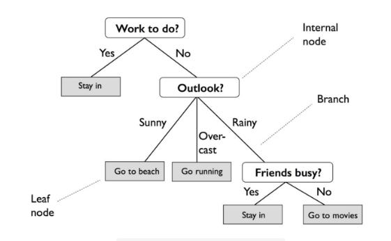
Based on entropy (the measure of variance within a class), DT creates a decision structure for interpreting patterns by classifying data into homogeneous or numerically relevant groups. Tree-like graphs are useful for displaying decision trees, and they’re easy for non-experts to understand.
It is quite different from an actual tree in that the “leaves” are located at the bottom, or foot, of the tree. Decision rules are expressed by the path from the tree’s root to its terminal leaf node. A branch represents the outcome of a decision or variable, and a leaf node represents a class label.
In order to implement DT, the following steps must be taken:
1 — Import libraries
2 — Import the dataset
3 — Convert non-numeric variables
4 — Remove columns
5 — Set X and y variables
6 — Set algorithm
7 — Evaluate
Exercise
Using the Advertising dataset, let’s use a decision tree classifier to predict a user’s click-through outcome.
Decision Trees Implementation
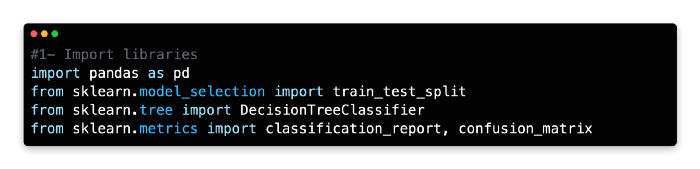
1: Import Libraries
As we will be predicting a discrete variable, we will use the classification version of the decision tree algorithm. In this example, we attempt to predict the dependent variable Clicked on Ad (0 or 1) by using the DecisionTreeClassifier algorithm from Scikit-learn. A classification report and a confusion matrix will be used to evaluate the model’s performance.
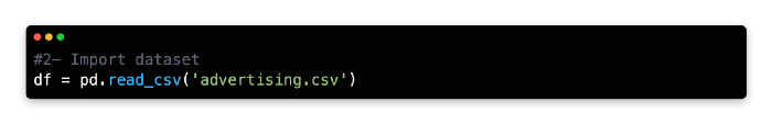
2: Import Dataset
Assign a variable name to the Advertising Dataset and import it as a data frame.
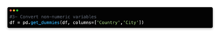
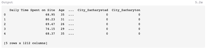
3: Convert Non-Numerical Variables
Numerical values can be obtained by encoding the Country and City variables one-at-a-time.
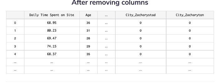
4: Remove Columns
Ad Topic Line and Timestamp are not relevant or practical for this model, so delete them.

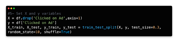
5: Set X and Y Variables
Our dependent variable (y) is the number of times people clicked on the ad, whereas our independent variables (X) are the remaining variables. In addition to Daily Time Spent on Site, Age, Area Income, Daily Internet Usage, Male, Country, and City, there are also independent variables.
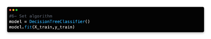
6: Set Algorithm
Assign DecisionTreeClassifier() to the variable model.
7: Evaluate
The training model should be tested on the X test data by using the predict function and a new variable name should be assigned.

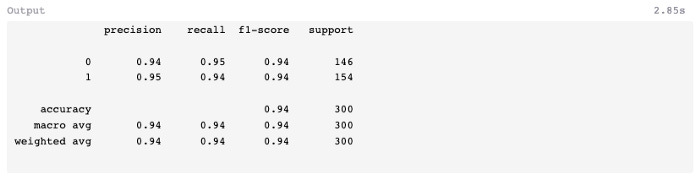
Nine false negatives and ten false positives were produced by the model. Next, let’s see if we can improve predictive accuracy using multiple decision trees.
Random Forest
In addition to explaining a model’s decision structure, decision trees can also overfit the model.
A decision tree decodes patterns accurately when using training data, but since it uses a fixed sequence of paths, it can make poor predictions when using test data. In addition to having only one tree design, this method is also limited in its ability to manage variance and future outliers.
Multiple trees can be grown using a different technique called RF to mitigate overfitting. For regression or classification, multiple decision trees are grown with a randomized selection of input data for each tree and the results are combined by averaging the outputs.
A randomized and capped variable is also chosen to divide the data. Every tree in the forest would look the same if a full set of variables were examined. Each split would allow the trees to select the optimal variable according to the maximum information gain at the subsequent layer.
However, random forests algorithm does not have a full set of variables to draw from, like a standard decision tree. Because random forests use randomized data and fewer variables, they are less likely to produce similar trees. Because random forests incorporate volatility and volume, they are potentially less likely to be overfitted and provide reliable results.
In order to implement RF, the following steps must be taken:
1 — Import libraries
2 — Import dataset
3 — Convert non-numeric variables
4 — Remove columns
5 — Set X and y variables
6 — Set algorithm
7 — Evaluate
Exercise
In this exercise, we are going to repeat the previous one, but using RandomForestClassifier from Scikit-Learn to learn the dependent and independent variables.
Implementation Of Random Forest
This part will familiarize you with the implementation steps of random forest.
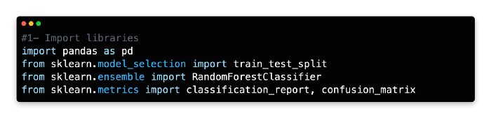
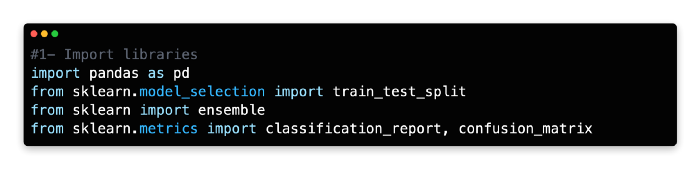
1: Import Libraries
In Scikit-learn, random forests can be built using either classification or regression algorithms. Scikit-learn’s RandomForestClassifier will be used here instead of RandomForestRegressor, which is used for regression.
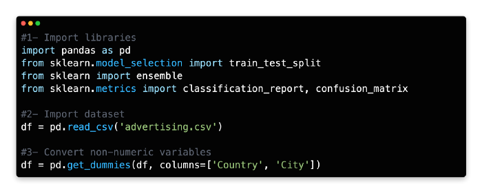
2: Import Dataset
Import the Advertising dataset.
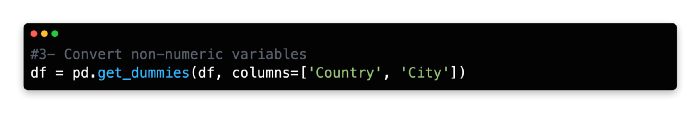
3: Convert non-numeric variables
Convert Country and City to numeric values using one-hot encoding.
4: Remove Variables
Data frame should be modified by removing the following two variables.

5: Set X and Y Variable
X and Y variables should be assigned the same values, and the data should be split 70/30.

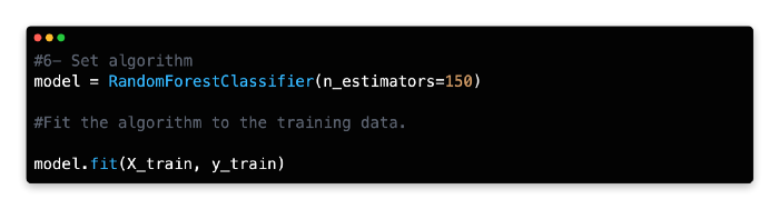
6: Set Algorithm
Give RandomForestClassifier a name and specify how many estimators it should have. In general, this algorithm works best with 100–150 estimators (trees).
7: Evaluate
The predict method can be used to predict the x test values and assign them to a new variable.
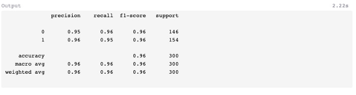
A comparatively low number of false-positives (5) and false-negatives (7) were found in the test data, and the F1-score was 0.96 instead of 0.94 in the previous exercise using a decision tree classifier.
Gradient Boosting
For aggregating the results of multiple decision trees, boosting is another regression/classification technique.
It is a sequential method that aims to improve the performance of each subsequent tree, rather than creating independent variants of a decision tree in parallel. Weak models are evaluated and then weighted in subsequent rounds to mitigate misclassifications resulting from earlier rounds. A higher proportion of items are classified incorrectly at the next round than at the previous round.
This results in a weaker model, but its modifications enable it to capitalize on the mistakes of the old model. Machine learning algorithms such as gradient boosting are popular due to their ability to learn from their mistakes.
GB implementation involves the following steps:
1 — Import libraries
2 — Import dataset
3 — Convert non-numeric variables
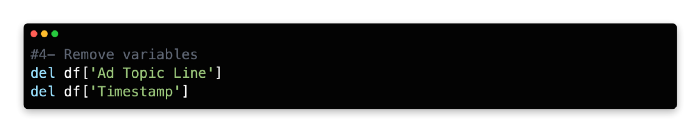
4 — Remove variables
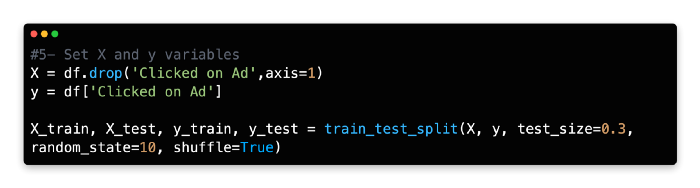
5 — Set X and y variables
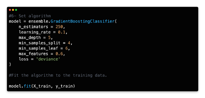
6 — Set algorithm
7 — Evaluate
Implementation Of Gradient Booster Classifier
In this third exercise, gradient boosting will be used to predict the outcome of the Advertising dataset so that the results can be compared with those from the previous two exercises.
The regression variant of gradient boosting will be familiar to readers of Machine Learning for Absolute Beginners Second Edition. Rather than using the classification version of the algorithm in this exercise, we will use a classification version which predicts a discrete variable using slightly different hyperparameters.
1: Import Libraries
Using Scikit-learn’s ensemble package, this model uses Gradient Boosting for classification.
2: Import Dataset
The Advertising dataset should be imported and assigned as a variable.

3: Convert Non Numerical Variables
4: Remove Variables
Remove the following two variables from the data frame.
5: Set X and Y Variables
X and Y variables should be assigned the same values, and data should be split 70/30.
6: Set Algorithm
Gradient Boosting Classifier should be given a variable name and its number of estimators should be specified. With a learning rate of 0.1 and a deviance loss argument, 150–250 estimators (trees) are a good starting point for this algorithm.
7: Evaluate
Assign the predicted X test values to a new variable using the predict method.
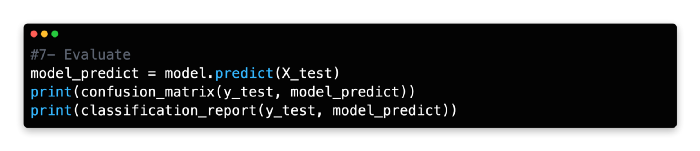
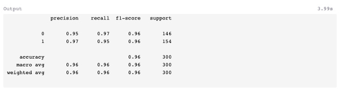
There was one less prediction error in this model than in random forests. In spite of this, the f1-score remains 0.96, the same as random forests, but better than the classifier which was developed earlier (0.94).
Implementation of Gradient Boosting Regressor
This exercise uses gradient boosting to estimate the nightly Airbnb rate for Berlin, Germany using a regression model. Then we’ll test a sample listing based on our initial model.
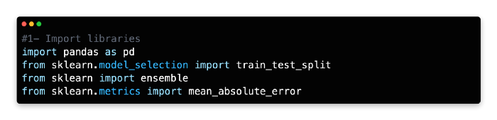
1: Import Libraries
Import the following libraries:
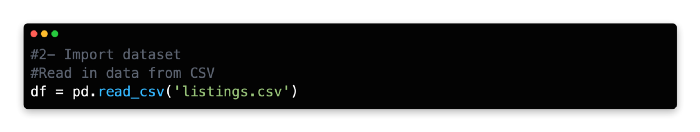
2: Import Dataset
Using the Berlin Airbnb dataset from Kaggle, we will perform this regression exercise.
The Berlin Airbnb dataset can be loaded into a Pandas dataframe by using the pd.read_csv command.
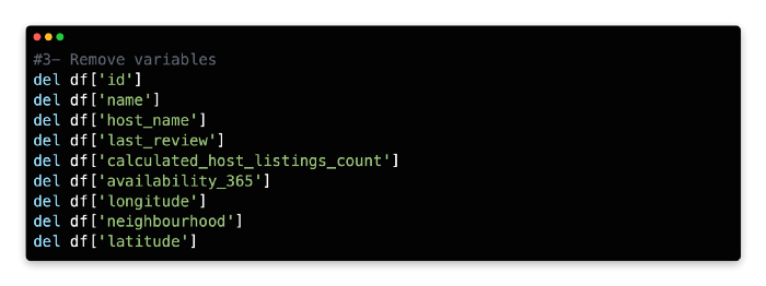
3: Remove Variable
It is not necessary to use all X variables for our model because some information overlaps between them (for example, host_name overlaps with host_id and neighborhood overlaps with neighborhood_group). Also, some variables are irrelevant, such as last_review, while others are discrete and difficult to parse, such as longitude and latitude.