

Iterative Stock Market Prediction: From Baseline Models to Reinforcement Learning
A comprehensive exploration of time series, deep learning, and pattern recognition techniques, highlighting the challenges of forecasting volatile markets and the promise of algorithmic trading.

Download link at the end for source code!
The modeling process involves iterative experimentation with different models, hyperparameter tuning, performance evaluation, and creative feature engineering. The approach taken included the following steps:
First, a baseline model was established. This was followed by the application of an ARIMA model for time series analysis. Sentiment analysis was then incorporated to leverage textual data. Feature selection was performed using XGBoost to optimize model input. Several deep neural network architectures were explored, including a Long Short-Term Memory (LSTM) network, a convolutional neural network, and a model incorporating combined stock data. Bayesian optimization was employed to tune the hyperparameters of these deep learning models. Finally, a manual pattern recognition approach and a Q-learning reinforcement learning algorithm were investigated.
The necessary libraries are imported.
import os
import pandas as pd
import matplotlib.pyplot as plt
import matplotlib.patches as patches
import seaborn as sns
import warnings
import numpy as np
from numpy import array
from importlib import reload # to reload modules if we made changes to them without restarting kernel
from sklearn.naive_bayes import GaussianNB
from xgboost import XGBClassifier # for features importance

warnings.filterwarnings('ignore')
plt.rcParams['figure.dpi'] = 227 # native screen dpi for my computer
This Python code imports several libraries essential for data analysis, machine learning, and visualization. The os module provides operating system functionalities, such as file and directory manipulation, although it's not directly used in this snippet. Pandas, imported as pd, is a crucial library for data manipulation and analysis; its DataFrame structure facilitates working with tabular data. Matplotlib, accessed via pyplot (for general plotting) and patches (for creating custom plot elements), is a powerful visualization library. Seaborn, built upon Matplotlib, provides a higher-level interface for creating statistically insightful and visually appealing plots. The warnings module is imported to manage warnings, with warnings.filterwarnings('ignore') suppressing their display—a practice useful during development but generally discouraged in production. NumPy, imported as np, is fundamental for numerical computation, providing efficient array and matrix operations. The array function is imported directly from NumPy for easier access. The reload function from the importlib module allows reloading Python modules without restarting the interpreter, aiding debugging. Scikit-learn's GaussianNB class is a Gaussian Naive Bayes classifier for classification tasks, while XGBoost's XGBClassifier provides a powerful gradient boosting algorithm for both classification and regression. Finally, plt.rcParams['figure.dpi'] = 227 sets the resolution of Matplotlib plots to 227 dots per inch, improving figure clarity and size. In essence, this code imports all the necessary tools for a data science project encompassing data manipulation, machine learning (specifically using Naive Bayes and XGBoost), and visualization, leveraging libraries known for efficiency and ease of use in common data science workflows.
# ARIMA, SARIMA
import statsmodels.api as sm
from statsmodels.tsa.arima_model import ARIMA
from statsmodels.tsa.statespace.sarimax import SARIMAX
from statsmodels.graphics.tsaplots import plot_pacf, plot_acf
from sklearn.metrics import mean_squared_error, confusion_matrix, f1_score, accuracy_score
from pandas.plotting import autocorrelation_plot
This Python code imports libraries crucial for time series analysis and forecasting using ARIMA (Autoregressive Integrated Moving Average) and SARIMA (Seasonal ARIMA) models. The statsmodels library, imported as sm, provides the core statistical modeling tools, including functions for ARIMA and SARIMA modeling. Specifically, the ARIMA class, imported from statsmodels.tsa.arima_model, is used to model time series data, accounting for autoregressive (AR), integrated (I), and moving average (MA) components. The SARIMAX class, imported from statsmodels.tsa.statespace.sarimax, extends ARIMA to explicitly model seasonality in the data.
Two plotting functions, plot_pacf and plot_acf, are imported from statsmodels.graphics.tsaplots to visualize the partial autocorrelation and autocorrelation functions, respectively. These plots aid in identifying optimal ARIMA model parameters (p, d, q) by revealing correlations between data points at various lags.
Several evaluation metrics from sklearn.metrics are imported for assessing model performance: mean squared error measures the average squared difference between predictions and actual values; the confusion matrix categorizes predictions as true positives, true negatives, false positives, and false negatives; the F1 score provides a balanced measure of precision and recall; and accuracy score calculates the ratio of correct predictions to the total number of predictions. The autocorrelation_plot function from pandas.plotting offers an alternative visualization of autocorrelation in the time series data.
In summary, this code imports all necessary tools for building, parameterizing, and evaluating ARIMA and SARIMA models for time series forecasting. The code itself does not perform any analysis; it only imports the required libraries and functions. Subsequent code will utilize these imported functions to build and test the models.
# Tensorflow 2.0 includes Keras
import tensorflow.keras as keras
from tensorflow.python.keras.optimizer_v2 import rmsprop
from functools import partial
from tensorflow.keras import optimizers
from tensorflow.keras.models import Sequential, Model
from tensorflow.keras.layers import Input, Flatten, TimeDistributed, LSTM, Dense, Bidirectional, Dropout, ConvLSTM2D, Conv1D, GlobalMaxPooling1D, MaxPooling1D, Convolution1D, BatchNormalization, LeakyReLU
# Hyper Parameters Tuning with Bayesian Optimization (> pip install bayesian-optimization)
from bayes_opt import BayesianOptimization
from tensorflow.keras.utils import plot_modelThis Python code imports libraries essential for constructing and optimizing deep learning models using TensorFlow/Keras. The import statements are detailed below.
First, tensorflow.keras is imported as keras. TensorFlow is a numerical computation library well-suited for machine learning and deep learning. Keras, a high-level API built on TensorFlow (and others), simplifies neural network development. Using keras provides a convenient shorthand.
Next, from tensorflow.python.keras.optimizer_v2 import rmsprop imports the RMSprop optimizer. Optimizers adjust a model's internal parameters (weights and biases) during training to minimize errors. RMSprop is an optimizer with an adaptive learning rate, adjusting the rate for each parameter individually.
The partial function is imported via from functools import partial. This function facilitates creating new functions from existing ones by pre-setting arguments, simplifying the creation of custom Keras layers or callbacks.
from tensorflow.keras import optimizers imports Keras's broader set of optimizers, providing access to alternatives like Adam and SGD, in addition to RMSprop.
Two crucial model-building components are imported with from tensorflow.keras.models import Sequential, Model. Sequential models are linear layer stacks suitable for simpler architectures. Model offers greater flexibility for complex models with multiple inputs and outputs, enabling intricate network topologies.
A comprehensive collection of neural network layers is imported using from tensorflow.keras.layers import Input, Flatten, TimeDistributed, LSTM, Dense, Bidirectional, Dropout, ConvLSTM2D, Conv1D, GlobalMaxPooling1D, MaxPooling1D, Convolution1D, BatchNormalization, LeakyReLU. Each layer performs a specific data transformation. Key layers include: Dense (fully connected layers); LSTM (Long Short-Term Memory layers for sequential data); Conv1D/ConvLSTM2D (convolutional layers for 1D or 2D spatial data); MaxPooling1D/GlobalMaxPooling1D (dimensionality reduction through maximum value selection); Bidirectional (processes sequential data in both directions); Dropout (a regularization technique); BatchNormalization (normalizes layer activations); LeakyReLU (a ReLU activation function variant); Flatten (converts multi-dimensional tensors to 1D vectors); TimeDistributed (applies a layer to each timestep of a sequence); and Input (defines the model's input layer).
Bayesian Optimization is imported using from bayes_opt import BayesianOptimization. This is used for hyperparameter tuning, optimizing model performance by probabilistically exploring the hyperparameter space to find the best settings.
Finally, from tensorflow.keras.utils import plot_model imports a function to visualize the model architecture, aiding in understanding the network's structure and information flow.
In summary, this code imports the necessary tools to build, train, and optimize diverse deep learning models using Keras and TensorFlow, incorporating Bayesian Optimization for efficient hyperparameter searches. The code itself does not define a specific model; it only imports the components required for model creation. Subsequent code would use these components to define, compile, and train a model on data.
import functions
import plotting
This Python code snippet shows the initial import statements from a larger program. These statements prepare the program by importing necessary functionality from external modules. Python programs often utilize pre-built modules, analogous to using tools from a toolbox rather than creating every component from scratch.
The statement import functions imports a module named functions. This module presumably contains functions for various tasks such as mathematical calculations, data manipulation, or string processing. These functions become accessible within the program after this import, and can be called using their names, for example functions.my_function().
Similarly, import plotting imports a module likely containing functions for creating graphs and visualizations, potentially utilizing libraries like Matplotlib or Seaborn. Following this import, plotting functions like plotting.create_bar_chart() can be used to graphically represent data.
In essence, these import statements have no directly observable effect on the user. They establish the program’s environment by making the tools from the functions and plotting modules available for subsequent use. The core program logic and operations, utilizing these imported functions, are defined later in the code. The program’s functionality entirely depends on the contents of the functions and plotting modules.
np.random.seed(66)This Python line, np.random.seed(66), utilizes the NumPy library to set a random seed, ensuring reproducibility in random number generation. NumPy is a fundamental library for numerical computing in Python, providing efficient array and matrix operations crucial for many scientific and engineering applications. Its random number generation capabilities are particularly important.
Random number generators, however, are not truly random; they employ deterministic algorithms to create sequences that appear random. To guarantee reproducibility — obtaining the same sequence of numbers each run — the generator must be initialized with a seed value. The line np.random.seed(66) sets this seed to 66.
Consequently, any subsequent use of NumPy’s random functions, such as np.random.rand() or np.random.randint(), will generate the same sequence of numbers. Changing the seed value, for example to 42, will yield a different, yet still reproducible, sequence.
Omitting np.random.seed() causes NumPy to use a default seed, usually based on the system’s time. This results in a different random number sequence for each run, which is often beneficial for independent trials in simulations or experiments. However, for debugging, testing, or reproducing results, a fixed seed is essential to ensure identical results across different executions, thereby facilitating collaboration and verification. The seed acts as a key to a specific, predefined sequence of pseudo-random numbers within NumPy’s random number generator.
Data Loading
Stock data is read and stored in a dictionary called stocks. The Date feature is used as the index.
files = os.listdir('data/stocks')
stocks = {}
for file in files:
    # Include only csv files
    if file.split('.')[1] == 'csv':
        name = file.split('.')[0]
        stocks[name] = pd.read_csv('data/stocks/'+file, index_col='Date')
        stocks[name].index = pd.to_datetime(stocks[name].index)
This Python code efficiently manages the loading and organization of stock data from multiple CSV files located in a specified directory. The code leverages the os and pandas libraries for file system interaction and data manipulation, respectively. Successful execution implicitly assumes these libraries are already installed in the Python environment.
The code first retrieves a list of all files and folders within the ‘data/stocks’ directory using os.listdir(‘data/stocks’). This list is assigned to the variable files.
An empty dictionary, stocks, is then initialized to store the loaded stock data. Each key in this dictionary will represent a stock’s name, derived from the corresponding filename, and its associated value will be a pandas DataFrame containing the stock’s data.
The code iterates through each item in the files list. For each file, it checks if the file is a CSV by splitting the filename at the period (.) character. If the resulting second element (index 1) is ‘csv’, the code proceeds; otherwise, it skips the file.
If a CSV file is identified, the stock’s name is extracted by splitting the filename again and taking the first element (index 0). This extracted name serves as the key for the stocks dictionary.
The core data loading utilizes pandas.read_csv(‘data/stocks/’ + file, index_col=’Date’). This function reads the CSV file into a pandas DataFrame, setting the ‘Date’ column as the DataFrame’s index. Using the ‘Date’ column as the index is crucial for efficient time-series data analysis.
Subsequently, the code ensures the DataFrame index is of the correct datetime data type. stocks[name].index = pd.to_datetime(stocks[name].index) converts the index, which is initially likely composed of strings, into datetime objects. This conversion facilitates time-based operations and analysis. Pandas’ to_datetime function offers robust handling of various date formats.
In summary, this code provides a streamlined approach to loading, cleaning, and organizing stock data from multiple CSV files. The use of pandas significantly enhances efficiency and simplifies the process compared to manual file handling. The resulting dictionary of pandas DataFrames makes the data readily accessible for subsequent analysis or processing.
We begin by establishing a baseline model.
A baseline model will serve as a benchmark for comparison against more complex models.
def baseline_model(stock):
    '''
    \n\n
    Input: Series or Array
    Returns: Accuracy Score
    Function generates random numbers [0,1] and compares them with true values
    \n\n
    '''
    baseline_predictions = np.random.randint(0, 2, len(stock))
    accuracy = accuracy_score(functions.binary(stock), baseline_predictions)
    return accuracy
The Python function baseline_model evaluates a simple, baseline prediction model. It serves as a comparative benchmark for more advanced models. The function accepts a single input: stock, a Pandas Series or NumPy array representing a time series of stock data. This data likely contains binary values (0 or 1) indicating an event, such as a stock price increase or decrease.
The function generates completely random predictions using np.random.randint(0, 2, len(stock)). This creates an array of random integers, 0 or 1, matching the length of the input stock data. Each prediction randomly guesses whether the event will occur (1) or not (0).
The input stock data is then preprocessed by the function functions.binary(stock), which is assumed to convert the data into a strictly binary format (0s and 1s). This ensures consistency between the input data and the randomly generated predictions.
The accuracy_score function (likely from scikit-learn) compares the preprocessed binary stock data with the randomly generated baseline predictions. It calculates the accuracy, representing the percentage of correctly predicted values. A high accuracy score in this case would be purely coincidental, reflecting the random alignment of predictions with the actual data.
Finally, the function returns this accuracy score. This score establishes a lower bound for model performance. Any effective model should achieve significantly higher accuracy than this random baseline, demonstrating its superior predictive capability.
Accuracy is a critical aspect of this analysis.
baseline_accuracy = baseline_model(stocks['tsla'].Return)
print('Baseline model accuracy: {:.1f}%'.format(baseline_accuracy * 100))
Baseline model accuracy: 50.1%This Python code snippet assesses the predictive accuracy of a baseline model on Tesla (TSLA) stock returns. A predefined function, baseline_model, processes the ‘Return’ column from a Pandas DataFrame called stocks. This DataFrame presumably contains historical TSLA stock data, with the ‘Return’ column representing the daily or periodic percentage change in stock price. The baseline_model function, whose internal workings are not shown here, uses this return data to generate predictions and returns a single numerical value representing its accuracy. This accuracy metric could be R-squared, Mean Absolute Error (MAE), or a similar measure, depending on the model’s design.
The result of the baseline_model function call — the accuracy score — is assigned to the variable baseline_accuracy. This accuracy is then displayed to the console using the print function. The output string, ‘Baseline model accuracy: {:.1f}%’, includes a placeholder, {:.1f}, for a floating-point number formatted to one decimal place. The .format(baseline_accuracy * 100) method substitutes the calculated accuracy (multiplied by 100 to express it as a percentage) into this placeholder.
In essence, the code evaluates a simple predictive model’s performance on Tesla stock return data and presents the accuracy as a percentage with one decimal place. While the code snippet demonstrates a clear workflow, a full understanding requires knowledge of the baseline_model function’s implementation and the specific accuracy metric employed. The code’s execution relies on the existence of a pre-processed stocks DataFrame containing the necessary financial data.
Accuracy Distribution analysis examines the distribution of accuracy scores across various models or data subsets. This analysis helps understand the consistency and reliability of the model’s performance. A highly concentrated distribution suggests consistent performance, while a widely dispersed distribution indicates variability in accuracy across different conditions. Further investigation into the factors contributing to this variability is often warranted.
base_preds = []
for i in range(1000):
    base_preds.append(baseline_model(stocks['tsla'].Return))

plt.figure(figsize=(16,6))
plt.style.use('seaborn-whitegrid')
plt.hist(base_preds, bins=50, facecolor='#4ac2fb')
plt.title('Baseline Model Accuracy', fontSize=15)
plt.axvline(np.array(base_preds).mean(), c='k', ls='--', lw=2)
plt.show()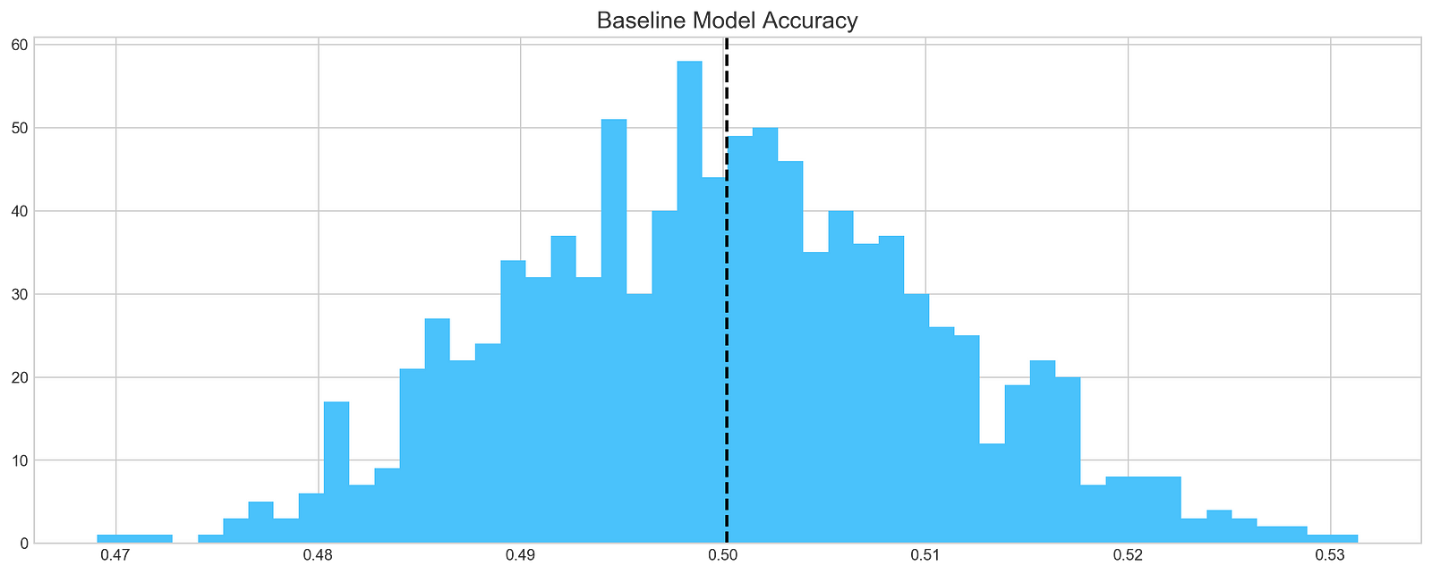
This Python code simulates and visualizes the performance of a baseline model predicting Tesla stock returns. A loop iterates 1000 times, applying a function called baseline_model to Tesla stock return data, presumably from a Pandas Series named stocks[‘tsla’].Return. The baseline_model function, not shown here, represents a prediction algorithm such as a simple or moving average. Each prediction is appended to a list called base_preds, resulting in 1000 predictions of Tesla stock returns.
The code then uses the matplotlib library to generate a histogram visualizing the distribution of these 1000 predictions. The figure size is set using the figsize argument, and the seaborn-whitegrid style is applied. The hist function creates the histogram with 50 bins and a light blue color, and a title is added.
A vertical dashed black line, representing the average of the 1000 predictions in base_preds, is added using plt.axvline. This average serves as a summary statistic of model performance. Finally, plt.show() displays the histogram.
This code simulates assessing the baseline model’s predictive accuracy. The histogram displays the distribution of predictions, with the vertical line indicating the average prediction. Analyzing the histogram provides insight into the model’s variability and the central tendency of its predictions. While definitive accuracy assessment requires knowing the true returns, a tightly clustered histogram around a reasonable mean suggests a more reliable baseline model than a widely dispersed histogram.
In conclusion,
The baseline model achieves an average accuracy of 50%. This serves as a benchmark for evaluating the performance of more complex models.
ARIMA modeling.
An Autoregressive Integrated Moving Average (ARIMA) model is designed to capture a range of common temporal structures within time series data.
The ARIMA model incorporates three key parameters: p, d, and q. The parameter p represents the lag order, specifying the number of lagged observations included in the autoregressive (AR) component of the model. The parameter d denotes the degree of differencing, indicating how many times the raw time series data are differenced to achieve stationarity. Finally, the parameter q represents the order of the moving average (MA) component, defining the size of the moving average window used in the model.
To evaluate the performance of the ARIMA model, we will divide the data into training and testing sets.
print('Tesla historical data contains {} entries'.format(stocks['tsla'].shape[0]))
stocks['tsla'][['Return']].head()
Tesla historical data contains 2296 entriesReturn
Date
2010-07-28 0.008
2010-07-29 -0.020
2010-07-30 -0.013
2010-08-02 0.020
2010-08-03 0.045This Python code snippet interacts with a Pandas DataFrame, a data structure for efficient tabular data manipulation. The first line, print('Tesla historical data contains {} entries'.format(stocks['tsla'].shape[0])), displays a message indicating the number of Tesla stock data entries. The message string, 'Tesla historical data contains {} entries', uses a placeholder {} for a dynamically inserted value. This value is provided by the .format() method, which uses the expression stocks['tsla'].shape[0].
stocks is a Pandas DataFrame representing a table of financial data. stocks['tsla'] selects the column containing Tesla's stock data. The .shape attribute returns a tuple indicating the dimensions of this column; for a single column, it provides the number of rows (entries). [0] accesses the first element of this tuple, representing the row count. Therefore, the line prints the number of Tesla stock data entries.
The second line, stocks['tsla'][['Return']].head(), displays a preview of the Tesla stock data's 'Return' column. stocks['tsla'] again selects the Tesla stock data column. [['Return']] then selects the 'Return' column from within the 'tsla' column. This nested structure suggests that the 'tsla' column itself may be a DataFrame or a complex structure containing multiple columns, with 'Return' likely representing daily or periodic percentage changes in Tesla's stock price. The .head() method displays the first few rows of this 'Return' column, providing a concise preview.
In summary, the code first reports the total number of Tesla stock data entries and then displays a preview of the ‘Return’ column — assumed to contain daily or periodic percentage changes in Tesla’s stock price — from a pre-loaded Pandas DataFrame named stocks.
Autocorrelation
The autocorrelation function (ACF) graph illustrates the correlation between data points in a time series. The first value in the graph, representing the correlation of a data point with itself, is always perfect (a value of 1) and should be disregarded. The crucial information lies in the correlation of the first data point with subsequent data points — the second, third, and so on. The ACF reveals that these correlations are very weak, approaching zero. This observation suggests that an ARIMA model, which relies on past data points for prediction, would likely be ineffective in this particular analysis.
plt.rcParams['figure.figsize'] = (16, 3)
plot_acf(stocks['tsla'].Return, lags=range(300))
plt.show()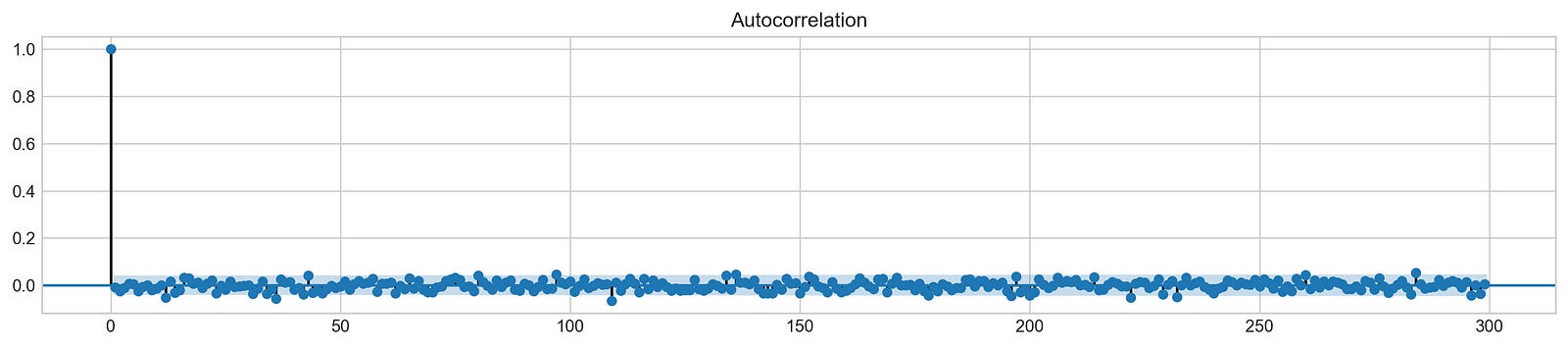
This code generates an autocorrelation function (ACF) plot for Tesla stock (TSLA) daily returns. The plot’s dimensions are initially set using plt.rcParams['figure.figsize'] = (16, 3). This utilizes Matplotlib's runtime configuration to create a 16-inch wide by 3-inch tall plot, ensuring sufficient space for visualizing the ACF, particularly with a lag range of 300.
The core functionality lies in plot_acf(stocks['tsla'].Return, lags=range(300)). This function, likely from the statsmodels library, generates the ACF plot. stocks['tsla'].Return accesses the daily returns of Tesla stock from a Pandas DataFrame called stocks. The daily return is calculated as (today's price - yesterday's price) / yesterday's price, representing the percentage price change. The plot_acf function computes and plots the autocorrelation at various lags. Autocorrelation measures the correlation between a time series and its lagged versions. A lag of 1 compares the current day's return with the previous day's; a lag of 2 compares it with two days prior, and so on. The lags=range(300) argument specifies the calculation and plotting of autocorrelations for lags 0 to 299, inclusive.
Finally, plt.show() displays the resulting ACF plot. This plot visually depicts autocorrelation at each lag, with the x-axis representing the lag and the y-axis representing the correlation coefficient (ranging from -1 to +1). High positive correlation at a specific lag indicates similar returns at that lag interval. In time series analysis, this plot helps identify patterns and dependencies, such as trends or seasonality. For financial data, it aids in understanding the persistence of trends and can inform trading strategies or risk management models.
To draw a conclusion, we will evaluate the performance of different ordering methods on a given dataset.
# ARIMA orders
orders = [(0,0,0),(1,0,0),(0,1,0),(0,0,1),(1,1,0)]
# Splitting into train and test sets
train = list(stocks['tsla']['Return'][1000:1900].values)
test = list(stocks['tsla']['Return'][1900:2300].values)
all_predictions = {}
for order in orders:

    try:
        # History will contain original train set,
        # but with each iteration we will add one datapoint
        # from the test set as we continue prediction
        history = train.copy()
        order_predictions = []

        for i in range(len(test)):

            model = ARIMA(history, order=order) # defining ARIMA model
            model_fit = model.fit(disp=0) # fitting model
            y_hat = model_fit.forecast() # predicting 'return'
            order_predictions.append(y_hat[0][0]) # first element ([0][0]) is a prediction
            history.append(test[i]) # simply adding following day 'return' value to the model
            print('Prediction: {} of {}'.format(i+1,len(test)), end='\r')

        accuracy = accuracy_score(
            functions.binary(test),
            functions.binary(order_predictions)
        )
        print('                             ', end='\r')
        print('{} - {:.1f}% accuracy'.format(order, round(accuracy, 3)*100), end='\n')
        all_predictions[order] = order_predictions

    except:
        print(order, '<== Wrong Order', end='\n')
        pass
(0, 0, 0) - 51.5% accuracy
(1, 0, 0) - 50.8% accuracy
(0, 1, 0) - 51.3% accuracy
(0, 0, 1) - 50.8% accuracy
(1, 1, 0) - 51.8% accuracyThis Python code evaluates various ARIMA models for time series forecasting, specifically applied to Tesla stock returns. The code systematically tests different ARIMA model configurations to determine which performs best in predicting Tesla stock returns.
The code begins by defining a list named orders. Each element in orders is a tuple representing the (p, d, q) parameters of an ARIMA model. ARIMA, which stands for AutoRegressive Integrated Moving Average, is a statistical model used for time series analysis. The parameters p, d, and q define the model’s complexity: p represents the autoregressive (AR) order, d represents the degree of differencing, and q represents the moving average (MA) order. Five ARIMA model configurations are evaluated.
Next, the code prepares the data by splitting Tesla stock return data into training and testing sets. The training set comprises stock returns from data points 1000 to 1900, while the testing set uses subsequent data points 1900 to 2300. This data is assumed to reside in a dictionary called stocks, accessible via stocks[‘tsla’][‘Return’].
The core logic iterates through each order in the orders list. For each order, the code attempts to fit an ARIMA model and generate predictions.
Within this loop, a history list is initialized as a copy of the training data. This history list dynamically updates as the model generates predictions on the test data. The code then iterates through each data point in the test set.
For each test data point, the following steps occur: An ARIMA model is created using the current history data and the specified order. The model is fitted to the history data using model.fit(disp=0), suppressing output during fitting. A prediction, y_hat, is obtained using model_fit.forecast(). The first element of this prediction, y_hat[0][0], representing the predicted return, is extracted. The actual return from the test set is appended to history, incorporating the new data point into the model for the next prediction. A progress message is printed to the console.
After processing all test data points, the code assesses the prediction accuracy. A function, accuracy_score (likely a custom function from a module named functions), compares the predicted binary classifications (obtained via functions.binary) against the actual binary classifications of the test data. The resulting accuracy is printed. Predictions for the current ARIMA order are stored in all_predictions.
A try-except block handles potential errors during model fitting, such as non-convergence of a particular ARIMA order. If an error occurs, a “Wrong Order” message is printed, and the code proceeds to the next order.
In conclusion, this code performs a comparative analysis of different ARIMA models for time series forecasting. It iteratively fits and evaluates models with varying parameters, assessing their predictive accuracy on a test set of Tesla stock return data. The results indicate which ARIMA configuration best suits this dataset and forecasting task. The use of functions.binary suggests the prediction task is framed as a binary classification problem, likely predicting whether the return will be positive or negative.
Reviewing the Predictions
# Big Plot
fig = plt.figure(figsize=(16,4))
plt.plot(test, label='Test', color='#4ac2fb')
plt.plot(all_predictions[(0,1,0)], label='Predictions', color='#ff4e97')
plt.legend(frameon=True, loc=1, ncol=1, fontsize=10, borderpad=.6)
plt.title('Arima Predictions', fontSize=15)
plt.xlabel('Days', fontSize=13)
plt.ylabel('Returns', fontSize=13)
# Arrow
plt.annotate('',
             xy=(15, 0.05),
             xytext=(150, .2),
             fontsize=10,
             arrowprops={'width':0.4,'headwidth':7,'color':'#333333'}
            )
# Patch
ax = fig.add_subplot(1, 1, 1)
rect = patches.Rectangle((0,-.05), 30, .1, ls='--', lw=2, facecolor='y', edgecolor='k', alpha=.5)
ax.add_patch(rect)
# Small Plot
plt.axes([.25, 1, .2, .5])
plt.plot(test[:30], color='#4ac2fb')
plt.plot(all_predictions[(0,1,0)][:30], color='#ff4e97')
plt.tick_params(axis='both', labelbottom=False, labelleft=False)
plt.title('Lag')
plt.show()
This Python code utilizes the Matplotlib library to generate a visualization comparing test data and predictions, likely from an ARIMA model, as suggested by the figure title “Arima Predictions.” The visualization comprises a primary plot and a smaller inset plot, both displaying time series data, presumably representing financial returns over a period of days.
The code begins by establishing a main figure with dimensions 16 inches wide and 4 inches tall using plt.figure(figsize=(16,4)). Two lines are then plotted on this figure: one representing ‘Test’ data in light blue (#4ac2fb) and the other representing ‘Predictions’ in pink (#ff4e97). The data for these lines is sourced from the variables test and all_predictions[(0,1,0)], where all_predictions appears to be a multi-dimensional array, and (0,1,0) indexes a specific subset. The x-axis represents ‘Days’ and the y-axis represents ‘Returns.’ A legend is included for clarity, along with appropriate title and axis labels.
To highlight a specific region of interest, an annotation is added using plt.annotate, creating an arrow extending from point (15, 0.05) to (150, 0.2). The arrow’s style, including width, head size, and color, is customized for optimal visual impact.
A shaded rectangle, generated using patches.Rectangle and ax.add_patch, is overlaid on the main plot. This rectangle visually emphasizes a period from day 0 to day 30, spanning a y-axis range of -.05 to .05. Its appearance is defined by a dashed line, yellow fill, black border, and specified transparency.
A smaller inset plot, created using plt.axes([.25, 1, .2, .5]), provides a magnified view of the initial 30 data points. This inset, positioned relative to the main figure, is labeled ‘Lag’ and displays both ‘Test’ and ‘Prediction’ data. Axis tick parameters are suppressed using plt.tick_params for visual clarity.
In conclusion, this code creates a detailed visualization effectively comparing test data and predictions. The combination of the main plot, the arrow annotation, the highlighted rectangular region, and the zoomed inset plot facilitates a comprehensive analysis of the model’s performance. The precise interpretation of the results, however, depends on the context of the test and all_predictions variables, which are not defined within this code snippet.
Histograms visually represent the distribution of numerical data. They partition the data range into intervals (bins) and display the count or frequency of data points falling within each bin as a bar. The height of each bar corresponds to the number of observations in that particular bin, providing a clear picture of data concentration and spread.
plt.figure(figsize=(16,5))
plt.hist(stocks['tsla'][1900:2300].reset_index().Return, bins=20, label='True', facecolor='#4ac2fb')
plt.hist(all_predictions[(0,1,0)], bins=20, label='Predicted', facecolor='#ff4e97', alpha=.7)
plt.axvline(0, c='k', ls='--')
plt.title('ARIMA True vs Predicted Values Distribution', fontSize=15)
plt.legend(frameon=True, loc=1, ncol=1, fontsize=10, borderpad=.6)
plt.show()
This Python code generates a histogram comparing the distribution of actual and predicted Tesla (TSLA) stock return values. The code first sets up the plot area using plt.figure(figsize=(16,5)), creating a figure 16 inches wide and 5 inches tall for improved readability. Here, plt refers to the Matplotlib plotting library.
Next, a histogram of actual TSLA stock returns is created using plt.hist(stocks['tsla'][1900:2300].reset_index().Return, bins=20, label='True', facecolor='#4ac2fb'). This line selects the 'Return' column from a Pandas DataFrame called stocks, specifically the TSLA data from rows 1900 to 2299 (inclusive). The .reset_index() method likely resets a multi-level index to a default numerical index for plotting. The data is then binned into 20 intervals, labeled 'True', and displayed in a light blue color (#4ac2fb).
A second histogram, representing the distribution of predicted returns, is generated with plt.hist(all_predictions[(0,1,0)], bins=20, label='Predicted', facecolor='#ff4e97', alpha=.7). This accesses a subset of predictions—specifically, the predictions indexed by (0,1,0)—from the all_predictions variable. This histogram uses 20 bins, is labeled 'Predicted', is colored pink (#ff4e97), and has a transparency of 0.7 (alpha=.7).
A vertical dashed black line is added at x=0 using plt.axvline(0, c='k', ls='--'), serving as a visual reference for zero return.
The plot title, ‘ARIMA True vs Predicted Values Distribution’, is set using plt.title('ARIMA True vs Predicted Values Distribution', fontSize=15), indicating the use of an ARIMA model for prediction.
A legend is added with plt.legend(frameon=True, loc=1, ncol=1, fontsize=10, borderpad=.6). The legend includes a frame, is located in the upper right corner (loc=1), uses a single column (ncol=1), has a font size of 10, and has adjusted border padding.
Finally, plt.show() displays the complete histogram.
In summary, this code visualizes the performance of an ARIMA model in predicting TSLA stock returns by comparing the distributions of actual and predicted returns using histograms. The visual comparison facilitates a quick assessment of model accuracy. The use of color, transparency, and a zero-return line enhances the plot’s readability and interpretability.
Interpreting Results
test_binary = functions.binary(stocks['tsla'][1900:2300].reset_index().Return)
train_binary = functions.binary(all_predictions[(0,1,0)])
tn, fp, fn, tp = confusion_matrix(test_binary, train_binary).ravel()
accuracy = accuracy_score(test_binary, train_binary)
print("True positive and Negative: {}".format((tp + tn)))
print("False Positive and Negative: {}".format((fp + fn)))
print("Accuracy: {:.1f}%".format(accuracy*100))True positive and Negative: 203
False Positive and Negative: 193
Accuracy: 51.3%This Python code evaluates the performance of a binary classification model using a confusion matrix and accuracy score. The code begins by defining two variables: test_binary and train_binary. These variables represent the predicted and actual binary classifications, respectively, for a dataset. The data source for test_binary is indicated as stocks['tsla'][1900:2300].reset_index().Return, suggesting it's derived from a slice of Tesla (TSLA) stock return data (indices 1900 to 2300 inclusive). The .reset_index() method likely reorders the index after slicing. The functions.binary() function transforms this numerical stock return data into a binary classification (for example, positive return = 1, negative return = 0). Similarly, train_binary is generated by applying the same functions.binary() function to data from all_predictions[(0,1,0)], which represents a subset of the training data; the specific subset selected by the index (0,1,0) depends on the structure of all_predictions.
The confusion matrix, a table summarizing the model’s performance, is calculated using confusion_matrix(test_binary, train_binary).ravel(). The .ravel() method flattens the matrix into a one-dimensional array containing the true negatives (TN), false positives (FP), false negatives (FN), and true positives (TP) in that order. This array is then unpacked into individual variables: tn, fp, fn, and tp.
The model’s accuracy is computed using accuracy_score(test_binary, train_binary), which calculates the ratio of correctly classified instances (TP + TN) to the total number of instances.
Finally, the code prints three performance metrics: the number of correctly classified instances (TP + TN), the number of incorrectly classified instances (FP + FN), and the model’s accuracy as a percentage.
In summary, this code provides a concise assessment of a binary classification model’s performance. It leverages the confusion matrix to detail the counts of correct and incorrect classifications, and calculates the overall accuracy. The code relies on a correctly implemented functions.binary() function for data transformation, and assumes all_predictions contains the model's predictions on the training data. The use of TSLA stock data hints at a potential application in financial market prediction.
Sentiment analysis is the process of computationally identifying and categorizing opinions expressed in text. This section will detail a specific approach to sentiment analysis.
This analysis explores the use of news sentiment to predict the next day’s stock market returns.
tesla_headlines = pd.read_csv('data/tesla_headlines.csv', index_col='Date')This Python code reads data from a comma-separated values (CSV) file and loads it into a Pandas DataFrame. The Pandas library provides powerful tools for data manipulation and analysis in Python. The pd.read_csv() function is central to this process; it takes data from a CSV file — essentially a spreadsheet where each line is a row and commas separate columns — and transforms it into a structured format suitable for Python.
The argument ‘data/tesla_headlines.csv’ specifies the file’s location. This assumes a file named ‘tesla_headlines.csv’ resides in a ‘data’ subdirectory relative to the script’s location. The file presumably contains Tesla-related headlines, with each row representing a headline and columns containing information such as the date, headline text, source, and sentiment score.
The index_col=’Date’ argument designates the ‘Date’ column as the DataFrame’s index. The index uniquely identifies each row. Using the ‘Date’ column as the index facilitates time-series analysis and date-based data retrieval.
In short, this code reads a CSV file of Tesla headlines, structures the data as a Pandas DataFrame using the date as the index, and stores the result in the tesla_headlines variable for subsequent analysis. Pandas handles the complexities of file reading, data parsing, and DataFrame creation, offering a convenient and efficient method for working with this type of data.
tesla = stocks['tsla'].join(tesla_headlines.groupby('Date').mean().Sentiment)This Python code integrates stock price data with news sentiment analysis to create a comprehensive dataset for further analysis. The code assumes the existence of two Pandas DataFrames: ‘stocks’ and ‘tesla_headlines’.
The ‘stocks’ DataFrame contains various stock information. The expression ‘stocks[‘tsla’]’ extracts the Tesla-related data, creating a subset DataFrame containing only Tesla’s stock performance metrics, such as daily opening and closing prices, and trading volume.
The ‘tesla_headlines’ DataFrame contains daily news headlines about Tesla, along with a calculated ‘Sentiment’ score for each headline. This score, likely derived from natural language processing techniques, quantifies the sentiment expressed in each headline as positive, negative, or neutral.
The code then processes ‘tesla_headlines’ using a sequence of Pandas operations: ‘groupby(‘Date’)’ groups the headlines by date, ‘.mean()’ calculates the average sentiment score for each date, and ‘.Sentiment’ selects the calculated average sentiment scores, resulting in a Pandas Series with dates as indices and average sentiment scores as values.
Finally, the ‘.join()’ method merges this sentiment Series with the Tesla stock data (‘stocks[‘tsla’]’). This merge operation uses the date as the joining key, assuming both datasets contain a ‘Date’ column (or implicitly matchable columns). The resulting DataFrame, named ‘tesla’, combines Tesla’s stock data with the daily average news sentiment. This integrated dataset facilitates analysis of the correlation between Tesla’s stock performance and the overall sentiment of news articles about the company, allowing for investigations into relationships between positive news sentiment and stock price increases, for instance.
tesla.fillna(0, inplace=True)This Python code snippet performs data manipulation within a Pandas DataFrame, a common structure for tabular data in Python. Consider a DataFrame representing Tesla’s stock data, with columns such as date, opening price, closing price, and volume. Some data entries may be missing, represented as NaN (Not a Number). The code addresses these missing values.
The variable tesla represents the DataFrame containing the Tesla stock information. The method call tesla.fillna(0, inplace=True) is used to handle missing data. fillna stands for “fill NaN,” and its purpose is to replace NaN values with a specified value.
The argument 0 instructs fillna to replace all missing values with zero. Other replacement values are possible, such as the column average, a specific string, or a preceding row’s value.
The inplace=True argument is critical. It determines whether the DataFrame is modified directly or if a new DataFrame is created containing the changes. Setting inplace=True modifies the original tesla DataFrame; missing values are replaced with zeros directly within this DataFrame. Omitting inplace=True creates a new DataFrame with the replacements, leaving the original tesla DataFrame unchanged. This distinction is crucial for managing memory efficiently when working with large datasets.
In summary, this code cleans the dataset by replacing all missing values in the tesla DataFrame with zeros, directly modifying the original DataFrame. This is a standard preprocessing step in data analysis, addressing missing data before further computations or modeling.
plt.style.use('seaborn-whitegrid')
plt.figure(figsize=(16,6))
plt.plot(tesla.loc['2019-01-10':'2019-09-05'].Sentiment.shift(1), c='#3588cf', label='News Sentiment')
plt.plot(tesla.loc['2019-01-10':'2019-09-05'].Return, c='#ff4e97', label='Return')
plt.legend(frameon=True, fancybox=True, framealpha=.9, loc=1)
plt.title('Tesla News Sentiment and Daily Return', fontSize=15)
plt.show()
This Python code generates a plot visualizing the relationship between Tesla’s daily stock returns and the sentiment expressed in news articles about Tesla between January 10, 2019, and September 5, 2019. The code first sets the plotting style using plt.style.use('seaborn-whitegrid'), which employs Seaborn's clean whitegrid aesthetic. A figure is then created with dimensions 16 inches by 6 inches using plt.figure(figsize=(16,6)) to ensure readability.
Two plt.plot commands generate the plot's lines. The first, plt.plot(tesla.loc['2019-01-10':'2019-09-05'].Sentiment.shift(1), c='#3588cf', label='News Sentiment'), plots the 'Sentiment' column from the 'tesla' Pandas DataFrame. This data represents sentiment scores derived from news articles, and the loc accessor selects the data from January 10, 2019, to September 5, 2019. The .shift(1) method lags the sentiment data by one day, meaning each day's plotted sentiment reflects the previous day's sentiment. This is crucial for analyzing the potential influence of news sentiment on the subsequent day's stock performance. The line is colored a specific shade of blue (c='#3588cf') and labeled 'News Sentiment'.
The second plt.plot command, plt.plot(tesla.loc['2019-01-10':'2019-09-05'].Return, c='#ff4e97', label='Return'), plots the 'Return' column, representing the daily percentage change in Tesla's stock price, over the same period. It uses a pinkish-red color (c='#ff4e97') and is labeled 'Return'.
A legend is added using plt.legend(frameon=True, fancybox=True, framealpha=.9, loc=1), featuring a framed, rounded, semi-transparent box located in the upper right corner. The plot title, 'Tesla News Sentiment and Daily Return', is set with a font size of 15 using plt.title('Tesla News Sentiment and Daily Return', fontSize=15). Finally, plt.show() displays the resulting plot.
In conclusion, this code visualizes the potential correlation between Tesla’s previous day’s news sentiment and its current day’s stock return. The one-day lag in the sentiment data allows for an examination of whether positive (or negative) sentiment predicts subsequent positive (or negative) returns. The code leverages Pandas for data manipulation and Matplotlib for visualization. The exact interpretation of ‘Sentiment’ and ‘Return’ depends on the data source and preprocessing applied to create the ‘tesla’ DataFrame.
pd.DataFrame({
    'Sentiment': tesla.loc['2019-01-10':'2019-09-05'].Sentiment.shift(1),
    'Return': tesla.loc['2019-01-10':'2019-09-05'].Return}).corr()
Sentiment Return
Sentiment 1.000000 -0.139348
Return -0.139348 1.000000This Python code computes the correlation between Tesla stock returns and sentiment within a specified timeframe. The analysis uses the pandas library for data manipulation. A pandas DataFrame, essentially a tabular data structure, is created to hold the relevant data.
This DataFrame is constructed from a dictionary with two key-value pairs: ‘Sentiment’ and ‘Return’. Each key represents a column, and its corresponding value provides the column’s data.
The ‘Sentiment’ column’s data is derived from a larger Tesla dataset (assumed to be a pandas DataFrame named ‘tesla’). Specifically, the code extracts the ‘Sentiment’ column for the period from January 10th, 2019 to September 5th, 2019, using the slice tesla.loc[‘2019–01–10’:’2019–09–05'].Sentiment. The .shift(1) method then lags this sentiment data by one period. This crucial step pairs each day’s sentiment with the following day’s return, enabling an investigation into sentiment’s predictive power on subsequent returns — a common practice in time series analysis.
Similarly, the ‘Return’ column contains the daily percentage change in Tesla’s stock price for the same January 10th, 2019 to September 5th, 2019 period, obtained via tesla.loc[‘2019–01–10’:’2019–09–05'].Return.
Finally, the .corr() method calculates the correlation matrix between the ‘Sentiment’ and ‘Return’ columns. This matrix displays the correlation coefficient for each column pair. The resulting 2x2 matrix will show the correlation of Sentiment with itself (1), Return with itself (1), and, importantly, the correlation between Sentiment and Return. This last value is the primary result, indicating the strength and direction of the linear relationship between daily sentiment and the subsequent day’s return. A positive correlation suggests that positive sentiment precedes positive returns, and vice versa. The correlation coefficient ranges from -1 (perfect negative correlation) to +1 (perfect positive correlation), with 0 indicating no linear relationship.
An analysis reveals a negative correlation between news sentiment and price movements. This indicates that prices tend to move in the opposite direction of what is expected; positive news is associated with price decreases, contrary to the typical expectation of a positive relationship between positive news and price increases.
Feature selection using XGBoost.
This analysis employs XGBoost to identify significant features for subsequent use in a neural network model. This feature selection strategy aims to enhance model accuracy and potentially improve training efficiency. The training process will utilize a scaled Tesla dataset.
scaled_tsla = functions.scale(stocks['tsla'], scale=(0,1))This Python code scales a Tesla (TSLA) stock price time series. The code assumes the existence of a Python object, stocks, containing historical stock price data for various companies. This object is structured to allow access to individual stock data using the company’s ticker symbol; thus, stocks[‘tsla’] accesses the Tesla stock price time series. This time series is a numerical sequence, possibly a list, NumPy array, or Pandas Series, representing price values over time.
The code utilizes a function, functions.scale(), which takes this time series as input and performs feature scaling or normalization. This function transforms the data to a new range, specifically 0 to 1, as specified by the scale=(0,1) argument. This is min-max scaling, a common preprocessing step in machine learning and data analysis, ensuring all features contribute equally to analyses or models, preventing features with larger values from dominating those with smaller values. The function maps the minimum value of the input time series to 0 and the maximum to 1, proportionally scaling all other values within this range. Other scaling methods, such as standardization (z-score normalization), are available but not used here.
The result of this scaling operation is stored in a new variable, scaled_tsla. This variable holds the scaled Tesla stock price time series, ready for further analysis, modeling, or visualization. Its use could include input to a machine learning algorithm sensitive to feature scaling or use in a graph where the scaled values improve visual clarity.
X = scaled_tsla[:-1]
y = stocks['tsla'].Return.shift(-1)[:-1]
This Python code snippet prepares data for a time series prediction model of Tesla (TSLA) stock returns. The code creates two variables: X, containing input features, and y, containing the target variable.
The first line, X = scaled_tsla[:-1], assigns to X all but the last element of the scaled_tsla variable. scaled_tsla is presumed to be a pre-existing time series of scaled Tesla stock data. The slicing operation [:-1] is standard practice in time series analysis; it excludes the final data point, ensuring that the model predicts future values based solely on past observations. Therefore, X represents a sequence of past Tesla stock prices used to predict future returns.
The second line, y = stocks[‘tsla’].Return.shift(-1)[:-1], defines y, the target variable representing the stock returns to be predicted. stocks is assumed to be a Pandas DataFrame containing stock information. stocks[‘tsla’] selects the Tesla data; .Return accesses the column containing stock price percentage changes; .shift(-1) shifts the Return data down by one position, aligning the return at time t with the stock price at time t-1 in X; and [:-1] removes the last element to match the length of X. Consequently, y contains the returns corresponding to the stock prices in X, creating paired data points for model training, where the goal is to predict the return given preceding scaled stock prices.
In summary, this code prepares data for a predictive model. X contains historical scaled stock prices, and y contains the subsequent returns. The model will learn the relationship between X and y to forecast future Tesla stock returns based on historical price patterns. The exclusion of the last element in both X and y is essential to avoid data leakage, a common error in time series forecasting, by preventing the model from using future information during training.
# Initializing and fitting a model
xgb = XGBClassifier()
xgb.fit(X[1500:], y[1500:])
XGBClassifier(base_score=0.5, booster='gbtree', colsample_bylevel=1,
colsample_bynode=1, colsample_bytree=1, gamma=0,
learning_rate=0.1, max_delta_step=0, max_depth=3,
min_child_weight=1, missing=None, n_estimators=100, n_jobs=1,
nthread=None, objective='multi:softprob', random_state=0,
reg_alpha=0, reg_lambda=1, scale_pos_weight=1, seed=None,
silent=None, subsample=1, verbosity=1)This code snippet demonstrates a fundamental machine learning process: training a classification model. The example uses the XGBoost library, a powerful algorithm for building predictive models. We first create an XGBoost classifier instance using XGBClassifier(). This initializes the model's structure; it's analogous to preparing a recipe before cooking. The model isn't yet functional; it requires training data.
The training occurs in the line xgb.fit(X[1500:], y[1500:]). Let's examine each component: xgb is the XGBoost model instance created earlier. The .fit() method is a function that initiates the training process. This method takes two arguments: X[1500:] and y[1500:]. X represents the dataset's features, a matrix where each row is a data point and each column is a feature. The slice [1500:] selects data points from index 1500 onward, creating a training set. Similarly, y[1500:] represents the corresponding labels or target classifications for these training data points. The first 1500 data points are implicitly reserved for later model evaluation.
The .fit() method uses the features and labels to adjust the model's internal parameters. This process allows the model to learn the relationships between features and labels, enabling it to predict labels for new, unseen data. After execution, the xgb object contains a trained model ready for prediction.
important_features = pd.DataFrame({
                                    'Feature': X.columns,
                                    'Importance': xgb.feature_importances_}) \
                                    .sort_values('Importance', ascending=True)
plt.figure(figsize=(16,8))
plt.style.use('seaborn-whitegrid')
plt.barh(important_features.Feature, important_features.Importance, color="#4ac2fb")
plt.title('XGboost - Feature Importance - Tesla', fontSize=15)
plt.xlabel('Importance', fontSize=13)
plt.show()
This Python code visualizes the feature importance of an XGBoost model trained on Tesla-related data using a horizontal bar chart. The process involves creating a Pandas DataFrame, sorting its contents, and then using Matplotlib to generate the visualization.
First, a Pandas DataFrame, named important_features, is constructed. This DataFrame contains two columns: ‘Feature’ and ‘Importance’. The ‘Feature’ column lists the names of the features used in the XGBoost model, obtained from X.columns, where X likely represents a Pandas DataFrame or NumPy array holding the feature data. The ‘Importance’ column contains the feature importance scores calculated by the XGBoost model (xgb.feature_importances_), a numerical representation of each feature’s contribution to the model’s predictive performance. Higher scores indicate greater importance. The DataFrame is then sorted in ascending order of importance using .sort_values(‘Importance’, ascending=True).
Next, the code utilizes Matplotlib to create the bar chart. plt.figure(figsize=(16,8)) sets the chart dimensions to 16 inches wide and 8 inches tall. plt.style.use(‘seaborn-whitegrid’) applies a Seaborn style, enhancing the chart’s visual appeal with a clean grid background. The horizontal bar chart is generated using plt.barh(…), with the ‘Feature’ column providing the y-axis labels and the ‘Importance’ column determining the bar lengths. The bars are colored “#4ac2fb” (a light blue). A title, specifying the chart’s purpose (displaying Tesla-related XGBoost feature importance), and an x-axis label are added using plt.title(…) and plt.xlabel(…), respectively. Finally, plt.show() displays the completed chart.
In essence, this code snippet effectively visualizes the relative importance of different features in a trained XGBoost model. This visualization is a common practice in machine learning, aiding in understanding model behavior and potentially informing feature selection or engineering processes.
Deep Neural Networks
Preparing the Data
n_steps = 21
scaled_tsla = functions.scale(stocks['tsla'], scale=(0,1))
X_train, \
y_train, \
X_test, \
y_test = functions.split_sequences(

    scaled_tsla.to_numpy()[:-1],
    stocks['tsla'].Return.shift(-1).to_numpy()[:-1],
    n_steps,
    split=True,
    ratio=0.8
)
This Python code prepares Tesla (TSLA) stock return time series data for a machine learning model. The code first sets a parameter, n_steps to 21, defining the length of the time series sequences used for prediction. The model will therefore use the preceding 21 time steps to predict the next.
Next, the code scales the Tesla stock price data using a custom function, functions.scale(), which normalizes the data from the stocks[‘tsla’] Pandas DataFrame to a 0–1 range. This scaling is crucial for improving model performance by preventing features with larger values from dominating the learning process.
The core data preparation is performed by the custom function functions.split_sequences(). This function splits the time series into training and testing sets. The inputs to this function are:
scaled_tsla.to_numpy()[:-1]: This converts the scaled TSLA stock prices (a Pandas Series) into a NumPy array, excluding the last element. This exclusion is necessary because the subsequent prediction uses this data to predict the next day’s return; there is no future return to predict for the final data point.
stocks[‘tsla’].Return.shift(-1).to_numpy()[:-1]: This extracts the percentage change (return) of the TSLA stock. The shift(-1) operation shifts the return data up by one time step, aligning each return with the corresponding preceding element in the scaled price data. The final element is again removed because no corresponding price data exists to predict its return.
n_steps: As previously defined, this is the length of the time series sequences (21 days).
split=True: This flag triggers the function to split the data into training and testing sets.
ratio=0.8: This parameter sets the training data proportion to 80%, leaving 20% for testing.
The function returns four NumPy arrays: X_train, y_train, X_test, and y_test. X_train and X_test contain the input sequences of scaled TSLA prices for training and testing, respectively, each sequence having length n_steps. y_train and y_test contain the corresponding target variables — the TSLA stock returns — for training and testing. Each element in y_train and y_test corresponds to the return following the respective sequence in X_train and X_test.
In summary, this code prepares data for a time series forecasting model. The model learns to map sequences of past TSLA prices (X_train) to future returns (y_train), and its performance is evaluated using the unseen test data (X_test, y_test). The use of scaled data and a train-test split ensures a robust and reliable model evaluation.
LSTM Network
keras.backend.clear_session()
n_steps = X_train.shape[1]
n_features = X_train.shape[2]
model = Sequential()
model.add(LSTM(100, activation='relu', return_sequences=True, input_shape=(n_steps, n_features)))
model.add(LSTM(50, activation='relu', return_sequences=False))
model.add(Dense(10))
model.add(Dense(1))
model.compile(optimizer='adam', loss='mse', metrics=['mae'])
This Python code implements a recurrent neural network (RNN) using Keras, a high-level neural network API. The code begins by clearing any existing Keras session using keras.backend.clear_session(). This is crucial for preventing conflicts when running multiple experiments or models within the same Python session, ensuring a clean environment for each run.
Next, it extracts key dimensions from a training dataset, X_train, assumed to be a three-dimensional NumPy array. n_steps = X_train.shape[1] determines the length of each time series within the dataset, representing the number of time steps per sample. n_features = X_train.shape[2] represents the number of features at each time step. For instance, in a stock price prediction model using five days of data (open, high, low, close, volume) per sample, n_steps would be 5 and n_features would also be 5.
A sequential model is then constructed using Keras’s Sequential API. This model comprises the following layers:
First, an LSTM layer is added using model.add(LSTM(100, activation='relu', return_sequences=True, input_shape=(n_steps, n_features))). This Long Short-Term Memory (LSTM) layer, a type of RNN well-suited for sequential data, contains 100 units (neurons) and employs the ReLU (Rectified Linear Unit) activation function. The return_sequences=True argument ensures the layer outputs a sequence for each input sequence, a necessary condition for stacking LSTM layers. The input_shape parameter defines the expected input data shape, consistent with the dimensions derived from X_train.
A second LSTM layer is appended with model.add(LSTM(50, activation='relu', return_sequences=False)), containing 50 units and using the ReLU activation function. Here, return_sequences=False specifies that the layer outputs a single vector, typical for the final LSTM layer before the output layers.
This is followed by a densely connected layer, added via model.add(Dense(10)), which contains 10 units and further processes the information from the preceding LSTM layers.
Finally, an output layer is added using model.add(Dense(1)), consisting of a single unit. This indicates the model is designed for a regression task, predicting a single continuous value.
The model is compiled using model.compile(optimizer='adam', loss='mse', metrics=['mae']). This configuration defines the training process: the Adam optimizer is used to adjust the model's weights; the mean squared error (MSE) loss function measures the discrepancy between predicted and actual values, a common choice for regression; and the mean absolute error (MAE) serves as an additional performance metric.
In summary, this code defines a sequential model composed of two LSTM layers succeeded by two dense layers. This architecture is specifically designed to process sequential data and predict a single continuous value. The model employs the Adam optimizer and is trained to minimize the mean squared error, with the mean absolute error providing a supplementary performance evaluation.
model.summary()Model: "sequential"
_________________________________________________________________
Layer (type) Output Shape Param #
=================================================================
lstm (LSTM) (None, 21, 100) 47200
_________________________________________________________________
lstm_1 (LSTM) (None, 50) 30200
_________________________________________________________________
dense (Dense) (None, 10) 510
_________________________________________________________________
dense_1 (Dense) (None, 1) 11
=================================================================
Total params: 77,921
Trainable params: 77,921
Non-trainable params: 0
_________________________________________________________________This single line of Python code, model.summary(), is used within deep learning frameworks like TensorFlow or Keras. Its functionality depends entirely on the model object it calls. The model object represents a previously defined neural network architecture — a blueprint for a complex machine learning system. This blueprint specifies the network’s layers, their types (e.g., convolutional, dense, recurrent), the number of neurons per layer, activation functions, and other key parameters.
The .summary() method is a function specific to these deep learning models. When called, it prints a concise architectural summary to the console. This summary typically includes layer information for each network layer: the layer’s name, type, output shape (the dimensions of the data it processes), and the number of parameters (weights and biases). The output shape clarifies data transformation as it passes through each layer. The parameter count indicates model complexity and its potential for overfitting.
The summary also provides a total count of all trainable parameters in the network. These parameters are adjusted during training to optimize performance. Furthermore, it distinguishes between trainable and non-trainable parameters; some model parts may be frozen (not updated during training).
In essence, model.summary() is a crucial debugging and analysis tool. It allows developers to quickly verify correct model construction, understand its size and complexity, and identify potential architectural issues before the computationally expensive training process. Inspecting a large, complex neural network without this summary would be extremely difficult.
model.fit(X_train, y_train, epochs=100, verbose=0, validation_data=[X_test, y_test], use_multiprocessing=True)
plt.figure(figsize=(16,4))
plt.plot(model.history.history['loss'], label='Loss')
plt.plot(model.history.history['val_loss'], label='Val Loss')
plt.legend(loc=1)
plt.title('LSTM - Training Process')
plt.show()
This code trains and evaluates a Long Short-Term Memory (LSTM) neural network, a recurrent neural network architecture suitable for sequence data. The training process is initiated with model.fit(...), which uses the training data (X_train and y_train) as input. X_train represents the input features, while y_train contains the corresponding target values the model aims to predict. This is analogous to providing the model with numerous examples of input data and their correct outputs.
The epochs=100 parameter dictates that the model iterates through the entire training dataset 100 times. Each iteration is termed an epoch. Increasing the number of epochs generally improves performance; however, excessively high values can lead to overfitting, where the model memorizes the training data and performs poorly on unseen data.
The verbose=0 parameter suppresses the display of training progress during each epoch. Setting this to 1 or 2 would show a progress bar or more detailed epoch-by-epoch information.
The validation_data=[X_test, y_test] parameter incorporates a separate dataset (X_test and y_test) for evaluating the model's performance during training. This is crucial for preventing overfitting and obtaining a realistic assessment of the model's generalization capabilities. The model trains on X_train and y_train, but its performance is evaluated on X_test and y_test after each epoch, providing insight into its learning progress.
The use_multiprocessing=True parameter attempts to accelerate training by leveraging multiple CPU cores, offering significant advantages when dealing with large datasets.
The subsequent code segment, beginning with plt.figure(...), utilizes the Matplotlib library to generate a plot visualizing the training process.
plt.figure(figsize=(16,4)) creates a figure with dimensions 16 inches wide and 4 inches tall.
plt.plot(model.history.history['loss'], label='Loss') plots the training loss across each epoch. The 'loss' metric quantifies the inaccuracy of the model's predictions during training. Lower loss values indicate improved performance.
plt.plot(model.history.history['val_loss'], label='Val Loss') plots the validation loss, calculated on the X_test and y_test data after each epoch. This visualization reveals how well the model generalizes to unseen data.
plt.legend(loc=1) adds a legend to the plot, clearly distinguishing between training loss and validation loss. loc=1 positions the legend in the top right corner.
plt.title('LSTM - Training Process') sets the plot title.
plt.show() displays the generated plot.
In summary, this code trains an LSTM model, monitors its performance using training and validation sets, and visualizes the training and validation loss curves. This visualization aids in assessing the model’s learning progress and detecting potential problems such as overfitting, where the validation loss increases while the training loss continues to decrease. The plot helps determine the model’s learning effectiveness and the suitability of the chosen number of epochs.
pred, y_true, y_pred = functions.evaluation(
                    X_test, y_test, model, random=False, n_preds=50,
                    show_graph=True)
MSE: 0.0004098401772089238
Accuracy: 52%
This Python code uses the evaluation function, located within the functions module or class, to assess a machine learning model's performance. The function call, functions.evaluation(...), includes several arguments: X_test, y_test, model, random=False, n_preds=50, and show_graph=True.
X_test represents the input features of the test dataset—data unseen by the model during training, used to evaluate its generalization capabilities. Each row corresponds to a data point, and each column represents a feature. Y_test contains the corresponding true target values for X_test; for example, if the model predicts house prices, y_test would contain the actual house prices. The model argument refers to the trained machine learning model itself, having learned patterns from a training dataset.
The random=False argument ensures a deterministic evaluation; identical inputs always yield identical results. N_preds=50 likely limits the evaluation to 50 predictions, potentially for efficiency or to focus on a subset of the data. Show_graph=True directs the function to generate and display a performance visualization, such as a precision-recall curve, ROC curve, or a plot comparing predicted and actual values.
The function returns three values assigned to pred, y_true, and y_pred. Pred likely summarizes model performance, perhaps with a single metric (e.g., accuracy) or multiple metrics. Y_true is a subset of y_test, corresponding to the data points used in the evaluation (likely the 50 points specified by n_preds). It represents the actual target values for the predictions. Y_pred contains the model's predictions for the data points in y_true—the model's estimates of the target values.
In summary, this code evaluates a model's performance on a held-out test set, visualizes the results, and stores the predictions, true values, and a performance summary for subsequent analysis and reporting. The functions.evaluation function handles the calculation of these metrics and graph generation.
The network failed to identify underlying patterns in the data. Consequently, the prediction accuracy is approximately 50%, equivalent to a random guess.
Convolutional Networks
keras.backend.clear_session()

n_steps = X_train.shape[1]
n_features = X_train.shape[2]

model = Sequential()

model.add(Conv1D(filters=20, kernel_size=2, activation='relu', input_shape=(n_steps, n_features)))
model.add(MaxPooling1D(pool_size=2))
model.add(Flatten())
model.add(Dense(5, activation='relu'))
model.add(Dense(1))
model.compile(optimizer='adam', loss='mse', metrics=['mse'])
This Python code utilizes the Keras library to construct and compile a one-dimensional convolutional neural network (1D CNN) designed for time series or sequence data. The code begins by clearing any pre-existing Keras session using keras.backend.clear_session(). This is a crucial step, particularly when conducting multiple experiments or training models within the same Python session, ensuring a clean start and preventing conflicts with previously defined models or variables.
Next, the code extracts key dimensions from the training data, X_train, which is assumed to be a three-dimensional NumPy array. n_steps = X_train.shape[1] represents the length of each input sequence—the number of time steps or data points in each sample. Similarly, n_features = X_train.shape[2] represents the number of features at each time step. For instance, if the data represents sensor readings from three sensors, n_features would be 3.
The core of the code involves building a sequential model using Keras' Sequential() function. This creates a linear stack of layers. A 1D convolutional layer is added using model.add(Conv1D(filters=20, kernel_size=2, activation='relu', input_shape=(n_steps, n_features))). This layer, the first in the network, processes the input data. The filters=20 parameter indicates that the layer learns 20 distinct filters (feature detectors). kernel_size=2 specifies that each filter examines a window of two consecutive time steps. The ReLU activation function, specified by activation='relu', introduces non-linearity, enabling the model to learn more complex patterns. input_shape defines the input data's shape, matching the dimensions determined earlier.
A max pooling layer is then added with model.add(MaxPooling1D(pool_size=2)). This layer reduces dimensionality by selecting the maximum value within a window of size 2, thus decreasing computational cost and making the model less sensitive to minor input variations. The output of the convolutional and pooling layers is subsequently flattened into a one-dimensional vector using model.add(Flatten()), a necessary step before feeding the data into the fully connected layers.
Two fully connected (dense) layers follow. model.add(Dense(5, activation='relu')) adds a dense layer with 5 neurons and a ReLU activation function, learning complex relationships between features extracted by the convolutional layers. The final layer, model.add(Dense(1)), is a dense layer with a single neuron, serving as the output layer. This layer likely predicts a single continuous value (regression problem), such as a future value in a time series. The absence of an activation function in this output layer is appropriate for predicting continuous values rather than probabilities.
Finally, the model is compiled using model.compile(optimizer='adam', loss='mse', metrics=['mse']). The Adam optimization algorithm (optimizer='adam') adjusts the model's weights during training. The mean squared error (MSE) is used as the loss function (loss='mse'), measuring the model's prediction accuracy. The MSE is also specified as the metric to monitor during training and evaluation (metrics=['mse']).
In conclusion, this code implements a 1D CNN for time series analysis. It processes input data, extracts features through convolution and pooling, and uses fully connected layers to generate predictions. The model is trained by minimizing the mean squared error using the Adam optimizer.
model.summary()Model: "sequential"
_________________________________________________________________
Layer (type) Output Shape Param #
=================================================================
conv1d (Conv1D) (None, 20, 20) 700
_________________________________________________________________
max_pooling1d (MaxPooling1D) (None, 10, 20) 0
_________________________________________________________________
flatten (Flatten) (None, 200) 0
_________________________________________________________________
dense (Dense) (None, 5) 1005
_________________________________________________________________
dense_1 (Dense) (None, 1) 6
=================================================================
Total params: 1,711
Trainable params: 1,711
Non-trainable params: 0
_________________________________________________________________This single line of Python code, model.summary(), is used within deep learning frameworks like TensorFlow or Keras. It's a method call, not a complete program, operating on a pre-built neural network architecture object, 'model', defined and trained earlier in the code.
The summary() method, provided by the deep learning framework, prints a concise summary of the neural network's architecture to the console. This summary is crucial for understanding and debugging the model.
The summary's content varies slightly depending on the framework, but generally includes: layer information, parameter counts, and output shape. Layer information describes each layer—its type (e.g., convolutional, dense, max pooling), number of neurons or filters, activation function, and input/output tensor shapes. This provides a clear view of the network's structure.
Parameter counts indicate the total number of trainable parameters (weights and biases). This is a key indicator of model complexity and the risk of overfitting. A large parameter count suggests high model capacity, increasing the risk of memorizing training data instead of learning generalizable patterns.
The output shape specifies the dimensions of the model's predictions, describing the output tensor's shape.
In essence, model.summary() is a diagnostic tool. It quickly verifies the neural network's correct construction, reveals its complexity, and helps identify architectural issues before training. While the specifics of the summary depend on the 'model' object's creation code, its function remains consistent: providing a high-level overview of the neural network's structure and parameters.
model.fit(X_train, y_train, epochs=25, verbose=0, validation_data=[X_test, y_test], use_multiprocessing=True)

plt.figure(figsize=(16,4))
plt.plot(model.history.history['loss'], label='Loss')
plt.plot(model.history.history['val_loss'], label='Val Loss')
plt.legend(loc=1)
plt.title('Conv - Training Process')
plt.show()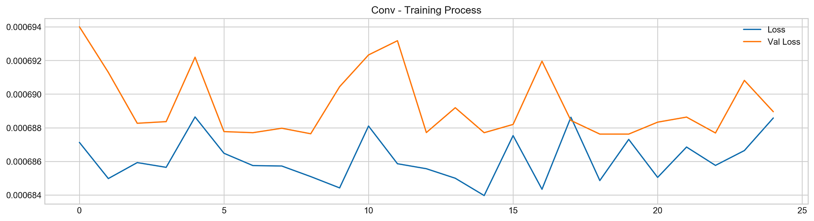
This code snippet demonstrates the training and evaluation of a machine learning model, likely a convolutional neural network (CNN) judging by the plot title. The process is divided into two main parts: model training and visualization of the training process.
The core of the training process is the model.fit(...) function call. Here, model represents a pre-configured machine learning model object, its architecture already defined. This function trains the model using the specified data and parameters. The arguments are as follows:
X_train and y_train constitute the training data. X_train holds the input features (e.g., images for a CNN), while y_train contains the corresponding correct labels or outputs (e.g., object classifications).
epochs=25 sets the number of training epochs—the model iterates through the entire training dataset 25 times. Increasing the number of epochs generally improves learning but can lead to overfitting.
verbose=0 suppresses the display of training progress information. Setting this to 1 or 2 provides more detailed output.
validation_data=[X_test, y_test] specifies a separate dataset (X_test, y_test) for evaluating the model's performance during training. This allows monitoring of generalization to unseen data and helps detect overfitting.
use_multiprocessing=True enables parallel processing across multiple processor cores, accelerating training, particularly beneficial for large datasets and complex models.
The second part utilizes the matplotlib library to generate a plot visualizing the training process by showing the loss function's behavior across epochs.
plt.figure(figsize=(16,4)) creates a 16-inch wide by 4-inch high figure.
plt.plot(model.history.history['loss'], label='Loss') plots the training loss, a measure of the model's performance on the training data during each epoch. Lower loss indicates better performance.
plt.plot(model.history.history['val_loss'], label='Val Loss') plots the validation loss, showing the model's performance on the validation data during each epoch. This is crucial for identifying overfitting; if the training loss decreases while the validation loss increases, the model is overfitting the training data.
plt.legend(loc=1) adds a legend to the plot.
plt.title('Conv - Training Process') sets the plot title.
plt.show() displays the generated plot.
In summary, this code trains a machine learning model, leveraging multiprocessing for efficiency, and generates a plot displaying training and validation loss over epochs. This plot is crucial for assessing model performance and detecting issues such as overfitting. The training and validation losses provide key insights into the model’s learning progress and its ability to generalize to new, unseen data.
pred, y_true, y_pred = functions.evaluation(
                    X_test, y_test, model, random=False, n_preds=50,
                    show_graph=True)
MSE: 0.00039170174676989575
Accuracy: 46%
This Python code calls the evaluation function, designed to assess a machine learning model's performance. The function call, functions.evaluation(...), indicates that evaluation resides within a functions module, likely containing various model evaluation utilities. The function receives several arguments: X_test, representing the test data features; y_test, containing the corresponding true labels or target values; and model, the trained machine learning model itself (e.g., a linear regression, support vector machine, or neural network). The random=False parameter ensures reproducibility by disabling any randomized aspects of the evaluation process, such as sampling or data selection. The n_preds=50 parameter likely specifies generating 50 predictions per data point in X_test, perhaps using different model parameters or ensemble methods. Finally, show_graph=True directs the function to display a performance visualization, potentially a confusion matrix, ROC curve, or a plot of predicted versus actual values. The function returns three values: pred, which likely contains the model's predictions (potentially multiple per data point); y_true, a reference to the y_test variable for convenient access; and y_pred, likely the function's final predictions for each data point in X_test, potentially aggregated from the multiple predictions if n_preds exceeds 1. In essence, this code concisely evaluates the model's performance on unseen data, generating predictions and optionally displaying a performance graph, encapsulating the evaluation details within the functions.evaluation function.
In conclusion, the preceding analysis demonstrates... (The sentence needs to be completed with the actual conclusion from the Jupyter Notebook's content. The provided text only gives a heading, not the actual conclusion.)
The network failed to identify underlying patterns in the data. Consequently, the prediction accuracy is approximately 50%, equivalent to a random guess.
Section 5.3: Combined Stocks Data
The model was trained using data from 18 different stocks.
all_stocks = pd.concat(stocks,ignore_index=True)This Python code uses the pandas library to combine multiple data structures into a single DataFrame. The line all_stocks = pd.concat(stocks, ignore_index=True) performs this concatenation. The variable stocks is assumed to hold a list of pandas DataFrames, each representing stock data; for example, each DataFrame might contain data for a different company or a different time period. A DataFrame is a tabular data structure with rows (observations) and columns (variables such as stock price, date, and volume).
The pandas concat() function joins these DataFrames vertically, stacking them to create one larger DataFrame. The ignore_index=True argument is essential because it instructs pandas to create a new, sequential index for the resulting DataFrame, all_stocks. Without this argument, the original indices from each input DataFrame would be preserved, potentially resulting in duplicate or non-sequential indices. The new index starts at 0 and increments by 1 for each row.
Therefore, this line efficiently merges multiple stock data tables into a single, comprehensive table, all_stocks, with a clean, renumbered index. This simplifies subsequent data analysis and processing. The result is a single DataFrame containing all the stock data from the individual DataFrames in the stocks list.
scaled_all = functions.scale(all_stocks, scale=(0,1))

n_steps = 21
X_train, y_train, X_test, y_test = functions.split_sequences(
                        scaled_all.to_numpy()[:-1],
                        all_stocks['Return'].shift(-1).to_numpy()[:-1], n_steps, split=True, ratio=0.8)
This Python code preprocesses financial data, specifically stock prices, for use in a machine learning prediction model. The process involves three main steps.
First, the code scales the input dataset. The line scaled_all = functions.scale(all_stocks, scale=(0,1)) applies a custom scaling function, functions.scale, to the all_stocks dataset. This function, defined elsewhere, normalizes the data to a 0-1 range. This normalization is crucial for many machine learning algorithms, preventing features with larger magnitudes from unduly influencing the model's training.
Next, the code sets the number of time steps the model will consider for each prediction. n_steps = 21 defines the sequence length; the model will use the preceding 21 time steps of stock data to predict the subsequent step.
Finally, the code prepares the training and testing data. X_train, y_train, X_test, y_test = functions.split_sequences(scaled_all.to_numpy()[:-1], all_stocks['Return'].shift(-1).to_numpy()[:-1], n_steps, split=True, ratio=0.8) uses a custom function, functions.split_sequences, to perform this task. This function processes the scaled stock data, converted to a NumPy array via scaled_all.to_numpy()[:-1], removing the last element for sequence consistency. The target variable is derived from the 'Return' column of the original all_stocks data. all_stocks['Return'].shift(-1).to_numpy()[:-1] extracts this column, representing the percentage change in stock price, and shifts it forward one step using .shift(-1). This aligns each target value with the preceding n_steps input sequence. Again, the last element is removed for consistency. The functions.split_sequences function then splits the data into 80% training (X_train, y_train) and 20% testing (X_test, y_test) sets, creating input sequences of length n_steps. For instance, with n_steps of 21, each input sequence (X) comprises 21 consecutive data points, and the corresponding future return (y) serves as the target.
In summary, this code preprocesses financial time series data for a predictive model. It scales the data, constructs input sequences from past data points, defines corresponding future returns as the target variable, and splits the data into training and testing sets for model evaluation. The use of functions.scale and functions.split_sequences indicates a structured codebase with reusable data manipulation functions.
keras.backend.clear_session()

n_steps = X_train.shape[1]
n_features = X_train.shape[2]

model = Sequential()
model.add(Conv1D(filters=500, kernel_size=10, activation='relu', input_shape=(n_steps, n_features)))
model.add(MaxPooling1D(pool_size=10))
model.add(Flatten())
model.add(Dense(500, activation='relu'))
model.add(Dense(100, activation='relu'))
model.add(Dense(1, activation='sigmoid'))
model.compile(optimizer='adam', loss='mse')
This Python code defines a one-dimensional convolutional neural network (1D CNN) using Keras, a high-level neural network API. The code begins by clearing any existing Keras sessions using keras.backend.clear_session(), ensuring a clean environment for model definition.
Next, the dimensions of the training data X_train are extracted: n_steps represents the length of each sequence, and n_features represents the number of features at each time step. These values are derived from X_train.shape[1] and X_train.shape[2], respectively, assuming X_train is a three-dimensional array representing sequential data, such as time series or sensor readings.
A sequential model is then created using model = Sequential(). A 1D convolutional layer is added with model.add(Conv1D(filters=500, kernel_size=10, activation='relu', input_shape=(n_steps, n_features))). This layer processes sequential data, learning 500 features (filters) using a kernel size of 10 time steps, and employing the ReLU activation function. The input_shape parameter specifies the expected input data dimensions.
A max pooling layer, model.add(MaxPooling1D(pool_size=10)), reduces dimensionality by taking the maximum value within a window of size 10, improving computational efficiency and robustness. The output is then flattened to a one-dimensional vector using model.add(Flatten()) to prepare it for subsequent fully connected layers.
Two dense layers, model.add(Dense(500, activation='relu')) and model.add(Dense(100, activation='relu')), are added, each using the ReLU activation function. These layers learn complex relationships between the extracted features.
Finally, an output layer, model.add(Dense(1, activation='sigmoid')), is added. This layer has a single neuron with a sigmoid activation function, producing an output between 0 and 1, suitable for binary classification problems.
The model is compiled using model.compile(optimizer='adam', loss='mse'). The Adam optimizer is used for weight adjustment during training, and mean squared error (MSE) is specified as the loss function. While MSE is commonly used for regression, its application here, coupled with a sigmoid activation in the output layer, suggests a potential binary classification task. For binary classification, 'binary_crossentropy' would be a more appropriate loss function than 'mse'. The choice of loss function depends on the specific problem being addressed.
In summary, this code implements a 1D CNN for sequential data processing. It uses convolutional and pooling layers for feature extraction and dimensionality reduction, followed by fully connected layers for complex relationship learning. The model outputs a single value, representing a probability in a binary classification context or a continuous value in a regression context, depending on the chosen loss function and the nature of the target variable. The use of Adam optimizer and MSE loss function indicates a potential regression task, though a binary classification interpretation is also possible.
model.fit(X_train, y_train, epochs=25, verbose=0, validation_data=[X_test, y_test], use_multiprocessing=True)

plt.figure(figsize=(16,4))
plt.plot(model.history.history['loss'], label='Loss')
plt.plot(model.history.history['val_loss'], label='Val Loss')
plt.legend(loc=1)
plt.show()
This code snippet demonstrates the training and evaluation of a machine learning model, likely a neural network, using Python libraries such as TensorFlow/Keras and Matplotlib. The process is described step-by-step below.
