

Linear Regression for Quant Trading: Building and Evaluating Predictive Models
An introduction to formulating, training, and diagnosing linear regression models using Python

Download the source using the URL at the end of this article!
Introduction to Linear Regression
Linear regression is a way to connect a continuous output, also called the response or dependent variable, with one or more input variables, often called predictors, features, or independent variables. It is built on the idea that the relationship has a linear form.
If the other features are held fixed, the effect of any one feature on the response follows a straight-line pattern.
The slope for that feature stays the same regardless of the values taken by the remaining variables.
Each feature contributes its own effect to the response, and those effects are combined additively, although interaction terms can also be introduced when needed.
Put differently, linear regression treats the response as something that can be described or estimated from a linear combination of the features, with the remaining difference attributed to random variation away from that pattern.
Imports and settings
import warnings
warnings.filterwarnings('ignore')
This step simply turns off warning messages for the rest of the session. Python libraries often emit warnings when something is deprecated, potentially unstable, or not quite ideal, and those messages can clutter the notebook without stopping the code from running. By setting the warning filter to ignore, the notebook keeps the display cleaner so the focus stays on the regression examples and results that come later. Since there is no saved output, nothing is printed here; the effect is purely behind the scenes, changing how warnings will be handled when later cells are executed.
%matplotlib inline

import numpy as np
import pandas as pd

import matplotlib.pyplot as plt
import seaborn as sns

import statsmodels.api as sm
from sklearn.linear_model import SGDRegressor
from sklearn.preprocessing import StandardScaler
This cell sets up the main tools needed for the rest of the notebook. The first line tells Jupyter to show plots directly inside the notebook rather than opening them in a separate window, which is why later visualizations will appear inline beneath the code that creates them. After that, the common data analysis libraries are loaded: one for numerical arrays, one for tabular data, and plotting libraries for making charts. The statistical modeling package is imported for ordinary least squares regression, and two scikit-learn classes are brought in as well, one for fitting a regression model with stochastic gradient descent and one for standardizing features before that model is trained.
There is no saved output from this cell because importing libraries and setting the plotting mode do not produce a visible result on their own. The effect is preparatory: it quietly configures the notebook environment so that later cells can generate data, fit regression models, and display figures without having to repeat these setup steps.
sns.set_style('whitegrid')
pd.options.display.float_format = '{:,.2f}'.format
The first line changes Seaborn’s plotting theme so that any charts drawn later will use a white background with light grid lines. That makes the plots easier to read, especially for regression examples where seeing the position of points, fitted lines, and residuals matters. The second line changes how pandas displays numbers in tables and summaries, telling it to show values with two decimal places and commas where appropriate. That affects the appearance of printed DataFrames and any tabular output that follows, giving the results a cleaner, more consistent look. Since this cell only adjusts display settings, it does not produce any visible output by itself; instead, it quietly prepares the notebook so later plots and tables are presented in a more polished format.
Basic Linear Regression
Create random sample data
x = np.linspace(-5, 50, 100)
y = 50 + 2 * x + np.random.normal(0, 20, size=len(x))
data = pd.DataFrame({'X': x, 'Y': y})
ax = data.plot.scatter(x='X', y='Y', figsize=(14, 6))
sns.despine()
plt.tight_layout()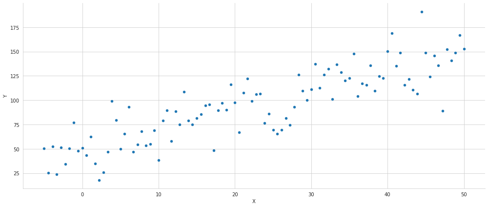
The goal here is to create a simple synthetic dataset for a regression example and immediately visualize it. The first line builds 100 evenly spaced x-values from -5 to 50, giving a smooth range of predictor values to work with. Next, the y-values are generated from a straight-line relationship with an intercept of 50 and a slope of 2, then random normal noise is added. That noise is important because it makes the data look like real observations instead of a perfectly clean line; the points will still follow an upward trend, but they will not all sit exactly on it.
Those two arrays are then packaged into a pandas DataFrame with columns named X and Y, which makes the data easier to plot and later reuse in model fitting. The scatter plot call draws Y against X, and the figure is made fairly wide so the trend is easy to see. The saved output shows the result of that plotting step: a cloud of points rising from left to right, with noticeable spread around the underlying line. That shape matches the way the y-values were constructed, because each point is based on a linear relationship with random variation added on top. The final two lines clean up the plot appearance by removing the top and right borders and tightening the layout so the chart fits neatly in the figure area.
Our basic one-predictor linear model is written as a response variable explained by a constant term, one feature, and an error term.
The error term represents the mismatch between the observed data and a perfectly straight-line relationship. Once the model is fitted to real observations, those mismatches are referred to as residuals.
Fit a simple regression model using statsmodels
The top section of the summary reports basic details about the data and model, including the estimation approach, how many observations and parameters are included, and the note that the reported standard errors are not adjusted for heteroskedasticity.
The center section lists the fitted coefficients, and these align closely with the way the synthetic data were created. As shown earlier, the same coefficient estimates in the middle of the summary can also be recovered using the OLS expression derived before.
X = sm.add_constant(data['X'])
model = sm.OLS(data['Y'], X).fit()
print(model.summary())
OLS Regression Results
==============================================================================
Dep. Variable: Y R-squared: 0.739
Model: OLS Adj. R-squared: 0.736
Method: Least Squares F-statistic: 277.6
Date: Thu, 15 Apr 2021 Prob (F-statistic): 2.39e-30
Time: 14:54:56 Log-Likelihood: -436.34
No. Observations: 100 AIC: 876.7
Df Residuals: 98 BIC: 881.9
Df Model: 1
Covariance Type: nonrobust
==============================================================================
coef std err t P>|t| [0.025 0.975]
------------------------------------------------------------------------------
const 49.5401 3.307 14.980 0.000 42.977 56.103
X 1.9942 0.120 16.661 0.000 1.757 2.232
==============================================================================
Omnibus: 0.389 Durbin-Watson: 1.721
Prob(Omnibus): 0.823 Jarque-Bera (JB): 0.103
Skew: -0.044 Prob(JB): 0.950
Kurtosis: 3.130 Cond. No. 47.6
==============================================================================
Notes:
[1] Standard Errors assume that the covariance matrix of the errors is correctly specified.The goal here is to fit a straight-line regression model to the existing data and then print the full statistical summary of that fit. The first step adds a constant column to the predictor values, which is how statsmodels includes an intercept term in the model. Without that extra constant, the regression would be forced to pass through the origin, which is not what we want for this example.
Next, the ordinary least squares model is built using the response values in Y and the predictor matrix that now contains both the intercept column and X. Fitting the model means statsmodels finds the line that minimizes the sum of squared residuals, so it chooses the intercept and slope that make the vertical prediction errors as small as possible overall.
The final line prints the model summary, and the saved output shows exactly the standard OLS report that statsmodels produces. The coefficient for const is about 49.54, and the coefficient for X is about 1.99, which matches the synthetic relationship used to generate the data very closely. That makes sense because the data were created from a line with an intercept near 50 and a slope near 2, plus some random noise. The R-squared value of 0.739 tells us that the fitted line explains a large share of the variation in Y, though not all of it, since the noise still adds scatter around the trend.
The other parts of the summary help assess how reliable the fit is. The small p-values for both coefficients indicate that the intercept and slope are statistically significant in the model. The t statistics and confidence intervals give another view of the same idea by showing that the estimated slope is clearly positive and far from zero. The diagnostics at the bottom, such as Omnibus, Jarque-Bera, Durbin-Watson, and the condition number, are there to check assumptions and possible issues in the residuals. Here they suggest nothing alarming, which is expected for a simple synthetic dataset built to follow a mostly linear pattern.
Check the calculation
beta = np.linalg.inv(X.T.dot(X)).dot(X.T.dot(y))
pd.Series(beta, index=X.columns)
const 49.54
X 1.99
dtype: float64The goal here is to calculate the regression coefficients directly from the ordinary least squares formula, rather than relying on a fitting routine. The expression first builds the matrix product of the predictors with themselves, takes its inverse, and then multiplies by the predictors and the response vector. That is the closed-form solution for linear regression, and it gives the coefficient values that minimize the sum of squared residuals.
The result is then wrapped in a Pandas Series so the numbers are easier to read, with the coefficient names taken from the columns of the design matrix. The saved output shows two estimated values: one for the intercept and one for the predictor X. The intercept is about 49.54 and the slope is about 1.99, which is very close to the data-generating pattern used earlier. That close match is exactly what we would expect if the synthetic data were built from a line with an intercept near 50 and a slope near 2, with only a little random noise added.
Show the fitted model and its residuals
data['y-hat'] = model.predict()
data['residuals'] = model.resid
ax = data.plot.scatter(x='X', y='Y', c='darkgrey', figsize=(14,6))
data.plot.line(x='X', y='y-hat', ax=ax);
for _, row in data.iterrows():
    plt.plot((row.X, row.X), (row.Y, row['y-hat']), 'k-')
sns.despine()
plt.tight_layout();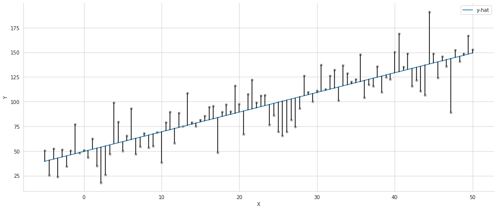
The goal here is to take the fitted linear regression model and turn it into a visual comparison between the observed data and the model’s predictions. First, the predicted values are stored in a new column called y-hat, and the model’s residuals are stored in another column. That makes it easy to inspect both the fitted response and the prediction errors alongside the original data.
Next, the data are plotted as a scatter plot with X on the horizontal axis and the observed Y values on the vertical axis. The points are drawn in dark grey so they serve as the raw observations. On top of that, the predicted values are plotted as a line using the y-hat column, which creates the blue fitted regression line seen in the output. Because the model is linear, the fitted values form a straight line that rises as X increases.
The loop that follows draws a vertical black segment for each observation, connecting the actual Y value to the predicted y-hat value at the same X position. These segments are the residuals visualized directly: the longer the line, the larger the prediction error for that point. In the saved figure, you can see some points sitting above the line and some below it, which is exactly what we expect from a regression fit with noise. The residual lines show that the model captures the overall upward trend, but individual observations still vary around that trend.
The final plotting calls clean up the appearance by removing the extra chart spines and tightening the layout so the figure looks neat and compact. The result is the displayed plot: a scatter of the observed data, the fitted regression line running through it, and residual segments showing how each point differs from the model’s prediction.
Multiple Linear Regression
When there are two predictors that are not dependent on one another, the regression equation expands to include both of them. In words, the response equals an intercept term, plus one coefficient multiplying the first variable, plus another coefficient multiplying the second variable, with an error term added at the end.
Create a fresh random dataset
## Create data
size = 25
X_1, X_2 = np.meshgrid(np.linspace(-50, 50, size), np.linspace(-50, 50, size), indexing='ij')
data = pd.DataFrame({'X_1': X_1.ravel(), 'X_2': X_2.ravel()})
data['Y'] = 50 + data.X_1 + 3 * data.X_2 + np.random.normal(0, 50, size=size**2)

## Plot
three_dee = plt.figure(figsize=(15, 5)).gca(projection='3d')
three_dee.scatter(data.X_1, data.X_2, data.Y, c='g')
sns.despine()
plt.tight_layout();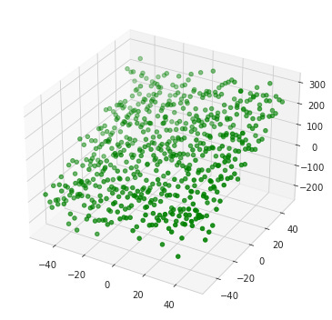
The purpose here is to build a synthetic three-dimensional data set for the multiple regression example and then display it as a scatter plot. It starts by choosing a grid size of 25, which controls how many values will be created along each predictor axis. Then two coordinate grids are generated with evenly spaced values from -50 to 50 for both X1 and X2. Using a mesh grid means every possible combination of the two predictor values is included, so the result is a full square grid of points rather than a random sample.
Those grid arrays are flattened and placed into a DataFrame so each row represents one observation with two predictors. After that, the response variable Y is created from a linear rule: a baseline of 50, plus one times X1, plus three times X2, with random noise added on top. That noise makes the relationship look realistic rather than perfectly flat and exact, while still preserving the overall linear trend.
Once the data are prepared, a 3D figure is created and the points are drawn as a green scatter plot. Each dot represents one synthetic observation in three-dimensional space, with X1 and X2 on the horizontal axes and Y on the vertical axis. The saved output shows exactly that: a cloud of green points spread across a tilted plane-like pattern. The upward tilt reflects the positive coefficients used to generate Y, and the scatter around that plane comes from the added random noise. The final styling steps remove extra plot borders and tighten the layout so the figure is cleaner and more compact.
X = data[['X_1', 'X_2']]
y = data['Y']
The purpose here is to separate the two parts of the regression dataset into inputs and target. The two predictor columns, X1 and X2, are collected together into a single feature table named X, while the response column, Y, is pulled out on its own and stored as y. Behind the scenes, this is just a tidy way of organizing the data so the regression model can treat the predictors as one matrix of explanatory variables and the outcome as the value it is trying to predict.
Nothing is printed or displayed because this step only assigns variables for later use. Its role is preparatory: once X and y have been defined, they can be passed into the fitting functions that estimate the regression relationship.
Fit a multiple regression model using statsmodels
The upper right section of the output reports the fit measures described earlier, together with the F test, which rejects the idea that every coefficient is zero and therefore uninformative. In the same area, the t statistics show that the intercept and both slope terms are, as expected, strongly significant.
The lower portion of the summary focuses on residual diagnostics. On the left, the skewness and kurtosis values are used when assessing whether the residuals follow a normal distribution. Both the Omnibus test and the Jarque Bera test do not provide enough evidence to reject the null hypothesis of normal residuals. The Durbin Watson statistic checks for serial dependence in the residuals; its value is close to 2, and with 2 predictors and 625 observations, it does not reject the assumption that the residuals are not serially correlated.
Finally, the condition number is a clue about multicollinearity. It is computed from the design matrix of the input data by comparing the square root of the largest eigenvalue with the square root of the smallest eigenvalue. When this value is greater than 30, it can indicate that multicollinearity may be a serious issue in the regression.
X_ols = sm.add_constant(X)
model = sm.OLS(y, X_ols).fit()
print(model.summary())
OLS Regression Results
==============================================================================
Dep. Variable: Y R-squared: 0.773
Model: OLS Adj. R-squared: 0.772
Method: Least Squares F-statistic: 1058.
Date: Thu, 15 Apr 2021 Prob (F-statistic): 7.00e-201
Time: 14:54:57 Log-Likelihood: -3321.0
No. Observations: 625 AIC: 6648.
Df Residuals: 622 BIC: 6661.
Df Model: 2
Covariance Type: nonrobust
==============================================================================
coef std err t P>|t| [0.025 0.975]
------------------------------------------------------------------------------
const 52.2837 1.970 26.537 0.000 48.415 56.153
X_1 0.9547 0.066 14.560 0.000 0.826 1.083
X_2 2.8610 0.066 43.631 0.000 2.732 2.990
==============================================================================
Omnibus: 7.484 Durbin-Watson: 2.050
Prob(Omnibus): 0.024 Jarque-Bera (JB): 7.714
Skew: -0.213 Prob(JB): 0.0211
Kurtosis: 3.338 Cond. No. 30.0
==============================================================================
Notes:
[1] Standard Errors assume that the covariance matrix of the errors is correctly specified.The purpose here is to fit a multiple linear regression model to the predictor data already stored in X and then immediately inspect the fitted results. The first step adds a constant column to the predictor matrix so the model can estimate an intercept term. Without that extra column, the regression would be forced through the origin, which would not match the usual linear regression setup used earlier.
After the intercept column is added, an ordinary least squares model is created with the response variable y and the augmented design matrix. When the model is fit, statsmodels solves for the coefficients that minimize the sum of squared residuals, meaning it chooses the linearly weighted combination of the predictors that comes closest to the observed target values overall. The next line prints the regression summary, which is what appears in the saved output.
The summary shows that the model explains a large share of the variation in the response, with an R-squared of 0.773. That means about 77 percent of the variation in Y is captured by the linear relationship with the two predictors. The adjusted R-squared is almost the same, which is a sign that both predictors are contributing useful information rather than just inflating the fit artificially. The very large F-statistic and tiny p-value indicate that the model as a whole is highly significant.
Looking at the coefficient table, the intercept is estimated at about 52.28, which is the predicted value of Y when both predictors are zero. The coefficient for X1 is about 0.95, and the coefficient for X2 is about 2.86. Those values are close to the underlying pattern used to generate the synthetic data, so the fitted model is recovering the expected relationship quite well, even though random noise keeps the estimates from being exact. The small standard errors and the near-zero p-values for both predictors show that each feature has a strong linear association with the response.
The lower part of the summary gives diagnostic information about the residuals and the overall model fit. The Durbin-Watson statistic is near 2, which suggests little evidence of autocorrelation in the residuals. The omnibus and Jarque-Bera tests, along with the skewness and kurtosis values, provide a rough check on whether the residuals look approximately normal; here they are close enough for a simple teaching example, though not perfectly ideal. The condition number is modest, which suggests the predictors are not causing severe numerical instability or multicollinearity in this setup.
Check the calculation
beta = np.linalg.inv(X_ols.T.dot(X_ols)).dot(X_ols.T.dot(y))
pd.Series(beta, index=X_ols.columns)
const 52.28
X_1 0.95
X_2 2.86
dtype: float64The goal here is to recover the regression coefficients directly from the ordinary least squares formula instead of relying on the model summary. First, the predictor matrix is transposed and multiplied by itself, which forms the central matrix used in the closed-form OLS solution. That matrix is then inverted, and the result is multiplied by the transpose of the predictors and the response values. Taken together, this applies the formula that gives the coefficient estimates minimizing the sum of squared residuals.
The result is stored as a set of fitted parameters, one for the intercept and one for each predictor. Turning those values into a labeled pandas Series makes the output easy to read because each number is paired with the name of the term it belongs to. The saved output shows an intercept of about 52.28, a coefficient of about 0.95 for X1, and a coefficient of about 2.86 for X2. Those values are very close to the synthetic relationship used to generate the data, which is why they look the way they do: the underlying data were built from a linear rule with a constant around 50 and slopes near 1 and 3, with a small amount of noise added.