


LSTM Model Trying To Predict Future Price Movement
LSTM Model Trying To Predict Future Price Movement
Coding a LSTM model from scratch to predict future price movements.

Download the code from the link in comment section.
Part 1: Setting Up Colab
#import libraries
from pandas_datareader import data
import matplotlib.pyplot as plt
import pandas as pd
import datetime as dt
import urllib.request, json
import os
import numpy as np
import tensorflow as tf
from sklearn.preprocessing import MinMaxScaler
This code includes several libraries and modules that are essential for analyzing and visualizing data, as well as for machine learning. The first library, pandas_datareader, allows us to collect financial information from various sources. The next library, matplotlib.pyplot, allows us to create visually appealing charts and graphs. Another library, pandas, helps with analyzing and manipulating data. The library datetime comes in handy when working with dates and times. To make HTTP requests, the library urllib.request is used. When dealing with JSON data, the library json is helpful. The library os allows us to interact with our operating system. For scientific calculations, the library numpy is used. For machine learning tasks, the library tensorflow is utilized. Finally, the library MinMaxScaler helps us scale data to prepare for machine learning models. All these libraries are imported so that we can effectively perform a variety of data analysis and machine learning tasks.
#declare name of your device and drive location select GPU
device_name = tf.test.gpu_device_name()
if device_name != '/device:GPU:0':
  raise SystemError('GPU device not found')
print('Found GPU at: {}'.format(device_name))
This piece of code sets the name for the device and chooses where it will be stored. It then double checks to make sure the name for the graphics card is correct, and if it isnt, it will display an error message. Once that is done, it will let you know that a graphics card has been found at the chosen location.
So here this time, I was thinking about using general electric dataset instead of usual amazon.
This new dataset is larger and it’s easier to observe their progress for longer time than amzn. If I need 900 data samples for training all I have to run testing on 180 days, but the rise of amazon has been around for 4 years to this date, so the data is limited especially for this kind of one day prediction and detecting price pattern.
This new dataset is larger this time and so I don’t have to worry about overfitting and I can focus more on training.
#Get your API data
df = pd.read_csv(os.path.join(f'{googlepath}','ge.us.txt'),delimiter=',',usecols=['Date','Open','High','Low','Close'])
This program helps us get important information from a website. The df variable is what we will use to store this information in a neat and organized way. To start, we bring in the pandas library using the shortcut pd. This library is often used to analyze and work with data in Python. Our next step is to use the read_csv function from pandas, which lets us take data from a CSV file. When using this function, we have to specify two things: where the file is located, and how the data is separated. We do this using os.path.join, which combines the googlepath and ge.us.txt variables to create a file path, and by saying that the data is split by commas. Finally, we tell the program which parts of the CSV file we want to keep, which in this case are the columns with the Date, Open, High, Low, and Close information. The data is then saved in the df variable so that we can use it later for more analyzing and organizing.
Find Average Price of High and Low Prices And Use That To Plot
plt.figure(figsize = (18,9))
plt.plot(range(df.shape[0]),(df['Low']+df['High'])/2.0)
plt.xticks(range(0,df.shape[0],500),df['Date'].loc[::500],rotation=45)
plt.xlabel('Date',fontsize=18)
plt.ylabel('avg Price',fontsize=18)
plt.show()
This program first makes a new picture with a size of 18 by 9 using the plt.figure function. Then, it draws a line graph by finding the average of the Low and High numbers for each row in the table. To make it easier to read, the plt.xticks function is used to show only every 500th date from the Date column. The labels for the x-axis and y-axis are also made bigger, with a font size of 18. To improve the look, the label text is tilted at a 45 degree angle. Finally, the graph is shown using the plt.show function.
# First calculate the average prices from the highest and lowest
high_prices = df.loc[:,'High'].as_matrix()
low_prices = df.loc[:,'Low'].as_matrix()
avg_prices = (high_prices+low_prices)/2.0
This program is finding the middle price from a set of data. It first looks for the column labeled High and puts that information into a collection called high_prices. Then, it does the same thing for the column labeled Low and stores that in a collection called low_prices. Next, the program adds up the numbers in both collections and divides them by 2 to get the average price. This average is then saved in a variable called avg_prices for future use. This process is repeated for each row of data, giving us an average price for each row.
Observations
Data Peaks around 1983 and then grows until the 2 crashes.
Calculating average prices Is somehow normalising the data and giving a much better picture than using only high prices or closing prices since it gives an idea about business around.
train = avg_prices[:11000]
test = avg_prices[11000:]
len(avg_prices)
This code generates two fresh variables, train and test, which hold distinct components of another variable called avg_prices. The train variable comprises of the first 11000 elements from the avg_prices variable, while the test variable includes all the remaining elements. Later, the length of the avg_prices list is determined, which tells us the total number of items in it.
Start Normalising Data
scaler = MinMaxScaler() #use mimaxscaler from scikitlearn to normalize data
train = train.reshape(-1,1)
test = test.reshape(-1,1)
This code uses the MinMaxScaler function from the scikitlearn library to make sure the data is in a consistent format. First, the function is given the nickname scaler. Then, the information from the train and test datasets is adjusted so it only has one column, which makes it easier for the scaler to work with. The scaler function then uses this data to change the values so they all fall between 0 and 1. This is helpful when dealing with different datasets that have different value ranges because it makes sure all the data is on the same scale. Normalizing also helps when there are different units of measurement.
Normalise average prices and trying to predict based on them instead of feature generation length of data is 12075.
window_size = 2500
for x in range(0,10000,window_size):
    scaler.fit(train[x:x+window_size,:])
    train[x:x+window_size,:] = scaler.transform(train[x:x+window_size,:])

scaler.fit(train[x+window_size:,:])
train[x+window_size:,:] = scaler.transform(train[x+window_size:,:])
First, we set a variable called window_size and give it the number 2500. This variable will help us make separate groups of data that dont overlap. Then, we use a for loop to go through numbers from 0 to 10000, with each group being 2500 numbers apart. This gives us groups of data that are each 2500 numbers long. Inside the loop, we use a scaler tool to adjust and change a part of the training data. The scaler tool takes the average and standard deviation of the data in each group. Then, it changes the data by subtracting the average and dividing by the standard deviation for each column. We put this new, changed data back in the same place as the original data, replacing it. The loop goes through this process for each group of data until it has gone through all of the training data. This makes sure that we change all of the data, not just one group. In the last part of the code, we use the scaler again to change any remaining data in the training set that wasnt included in the previous groups. This means now all of the data has been changed the same way and is ready for us to do more with it.
# Reshape both train and test data
train = train.reshape(-1)
First, the code takes the variable train and applies the reshape method to it, using the argument -1. This modifies the arrangement of the information stored in the variable. By using -1 as the argument, the code can determine the appropriate arrangement without needing specific instructions, since it depends on the amount of information present. This is particularly helpful when dealing with datasets of different sizes. As a result, the variables content is changed for both the train and test data, making them easier to handle and compare for future data examination.
Making this into a 2d shape train
# Normalize test data
test = scaler.transform(test).reshape(-1)
This piece of code works with a variable named test that supposedly holds some information. Next, it makes use of a method known as transform from an object referred to as scaler to alter the data in test. From what is understood, this scaler object helps make the data more uniform in some way, but the exact steps of this process are not specified. Once the alteration is complete, the outcome is reconfigured into a one-dimensional form using another method called reshape and then saved back into the variable test. This makes it easier to examine or carry out any additional actions on the standardized data.
EMA Averaging
EMA = 0.0 # keep EMA 0.0
ema2 = 0.1 # gamma is a variabe that can be multiplied with train
for i in range(11000):
  EMA = ema2*train[i] + (1-ema2)*EMA
  train[i] = EMA
In this code, we are setting up EMA and ema2, which are used to calculate an exponentially weighted average. We are starting with a certain set of values for EMA and ema2. Then, with a for loop, we are going through each element in train represented by i and calculating a new value for EMA. This new value takes into account the original value of EMA, as well as the value of gamma, which we can adjust. After each calculation, the loop continues to the next element, updating the overall EMA as it goes. Finally, we update the train array with the new EMA values, giving us a complete array of updated averages for the original data.
# Used for visualization and test purposes
all_avg_data = np.concatenate([train,test],axis=0)
This code helps combine two arrays, train and test, and create a new array called all_avg_data. The function used for this is concatenate, and it comes from the numpy library, which is used for doing math and science in Python. The goal of making this new array is to examine and experiment with something, possibly information or data from the original arrays. The axis=0 determines that the two arrays will be combined in the first row, so the new array will have the same columns as the original arrays combined. This code doesnt show any results, it simply makes a new array with the merged data for later use.
One Step Ahead Predictions Via Averaging
window_size = 100 # chose standard window size of 100
N = train.size
mse_err = []
_avg_pred = [] #create a list for average x, predictions and mse errors
_avg_x = []

for idx1 in range(window_size,N): #make a for loop where if the value is greater than size then use timedelta function for that 1 day

    if idx1 >= N:
        date = dt.datetime.strptime(k, '%Y-%m-%d').date() + dt.timedelta(days=1)
    else:
        date = df.loc[idx1,'Date']  #if not just find that value in the dataframe for the data and put it in date

    _avg_pred.append(np.mean(train[idx1-window_size:idx1])) #Keep apending values into into the lists
    mse_err.append((_avg_pred[-1]-train[idx1])**2)   #calculate mse errors
    _avg_x.append(date) #this is the x train for averages we will use to train

print('MSE error for standard averaging: %.5f'%(0.5*np.mean(mse_err)))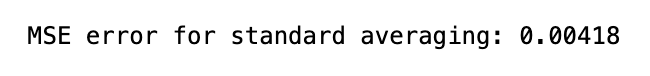
This piece of code is designed to figure out Mean Square Error MSE for a machine learning program. The first line determines a window size of 100. Then, the variable N is set to represent the number of data points in the training dataset. Next, three lists are made to hold the average x values, predictions, and MSE errors. The for loop goes through each data point in the training set, starting from the window size and going all the way to the end. During each iteration, it checks if the current index is the same or higher than the total number of data points. If it is, it uses the timedelta function to add one day to the current date. If not, it assigns the current dates value to the date variable. The next line adds the average of the previous data points to the avg_pred list. Then it calculates the MSE error by taking the difference between the current average prediction and the actual value, squaring it, and adding it to the mse_err list. Finally, the loop adds the current date to the avg_x list. As a final step, the code shows the MSE error, calculated through the standard averaging formula, which multiplies the average of squared errors by 0.5. Ultimately, this code measures MSE for a machine learning program using a window size of 100.
for range from 100 to size of train(11000) create the training data dates and then find their mean and append them to average predictions
else:
make a test set and then append all this to std_avg(all dates in this)
and:
calculate the mse_err
The above method is super awesome to calculate simple or standard averages. It uses timedelta to mainpulate date and push the date back to 1 day and add it to date along with datetime which strups the date and time from the given format.
plt.figure(figsize = (18,9))
plt.plot(range(df.shape[0]),all_avg_data,color='y',label='True')
plt.plot(range(window_size,N),_avg_pred,color='b',label='Prediction')
plt.xlabel('Date')
plt.ylabel('avg Price')
plt.legend(fontsize=18)
plt.show()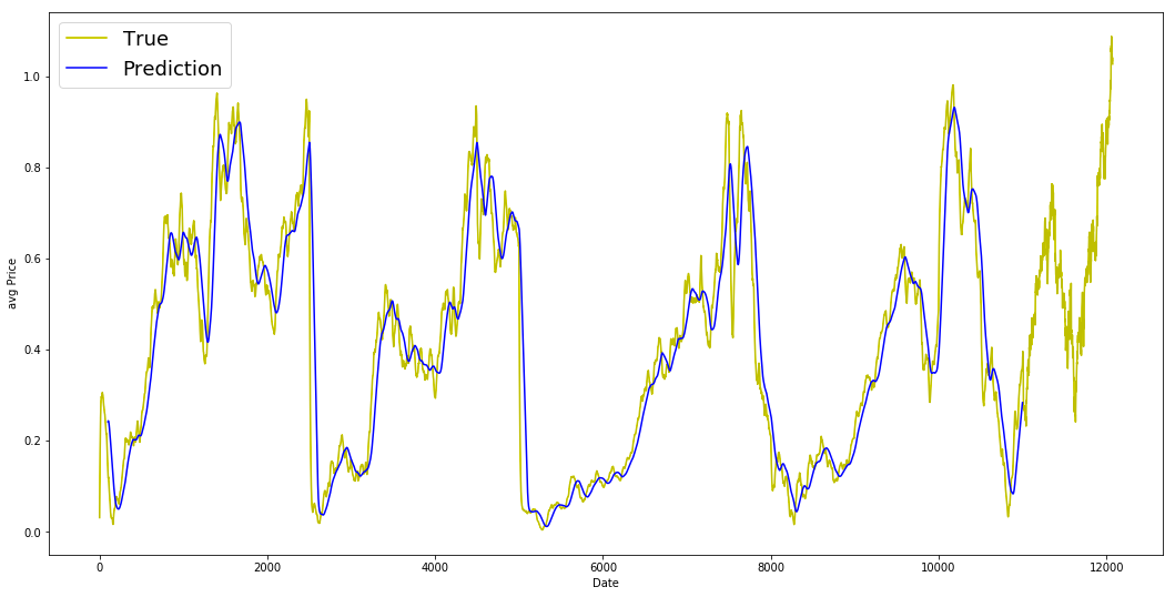
this code helps us see and compare the actual and predicted average data on a graph.
Everythign worked, Now let’s exponential moving average similar to what we tried in previous articles.
window_size = 100
N = train.size
mse_err = []
_avg_predictions_run = []
_avg_x_run = []


running_mean = 0.0 #the mean tat is calculates
_avg_predictions_run.append(running_mean)

decay = 0.5 # use this to average the running mean again;

for idx1 in range(1,N): #range from 1 to N-1

    running_mean = running_mean*decay + (1.0-decay)*train[idx1-1] #the remaining prob multiplied by the train sets data points
    _avg_predictions_run.append(running_mean)
    mse_err.append((_avg_predictions_run[-1]-train[idx1])**2) #make mse error with the help of train set
    _avg_x_run.append(date) #append the dates into the list

print('MSE error for EMA averaging: %.5f'%(0.5*np.mean(mse_err))) #Calculate MSE
The following code calculates the average and MSE Mean Squared Error values for a group of data points. First, it sets the window size to 100, which will be used in the calculation. Then, it determines the size of the training set and creates empty lists to store the MSE error, average predictions, and average x values. The initial running mean is set to 0.0 and stored in the list _avg_predictions. The decay value is then set to 0.5, which is used in the calculation of the average running mean. The code then loops through the training set from index 1 to N-1. Within the loop, the running mean is multiplied by the decay value and added to the data point at index idx1–1, which is the remaining probability multiplied by the data points. The updated running mean is appended to the list _avg_predictions. At the same time, the MSE error is calculated by subtracting the current running mean from the data point at index idx1, squaring the difference, and adding it to the mse_err list. The current date is also added to the list _avg_x. Finally, the code displays the MSE error for EMA Exponential Moving Average averaging by taking the average of the total MSE error.
MSE is great for EMA much better than simple average
plt.figure(figsize = (18,9))
plt.plot(range(df.shape[0]),all_avg_data,color='y',label='True Price Stock')
plt.plot(range(0,N),_avg_predictions_run,color='r', label='Prediction')
plt.xlabel('Date')
plt.ylabel('avg Price')
plt.legend(fontsize=18)
plt.show()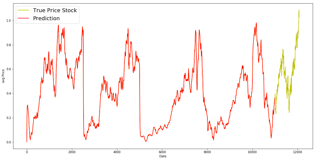
EMA is a great model for this dataset. Ideally the pattern of the True data should have been followed in the prediction model.
We coded from range to 1 to N-1 and put all the averaged values in the running mean. We used dense as 0.5 and then multiply it with the running average.