

Machine Learning with Numpy
Using scikit-learn, we’ll make predictions in this article. With scikit-learn, we will be able to predict accurately and quickly. Machine learning emphasizes measuring the ability to predict.

Iris Setosa, Iris Versicolor, and Iris Virginica flowers are included in the iris dataset, which consists of measurements.
Prediction strength will be measured by:
Testing data should be saved
Use only training data to build a model
Using the test set, measure the predictive power
There is only one categorical flower type in the prediction. A classification problem is one of these types of problems.
The best way to classify something is to ask, “Is it an apple or an orange?” Machine learning regression asks, “How many apples are there?” For regression, there can be 4.5 apples.
The four main categories of scikit-learn’s design are as follows:
Classification:
Non-text classification, like the Iris flowers example
Text classification
Regression
Clustering
Dimensionality reduction
An introduction to NumPy
Structured tables of data are a part of data science. Input tables for scikit-learn must be two-dimensional NumPy arrays. The numpy library will be explained in this section.
We will try a few operations on NumPy arrays. NumPy arrays have a single type for all of their elements and a predefined shape. Let us look first at their shape.
NumPy arrays’ dimensions and shapes
Import NumPy by following these steps:
Like Python’s range(10) method, create a NumPy array with 10 digits:
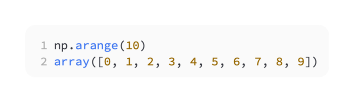
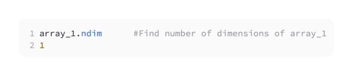
In this array, there is only one pair of brackets, similar to a Python list. One dimension means it has one dimension. Using the array, determine the shape:
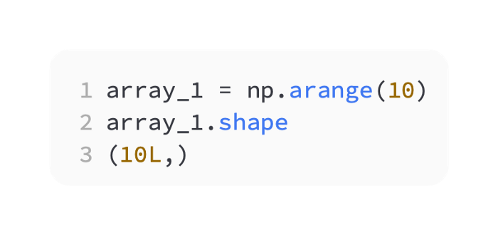
Shape is the data attribute of the array. In this case, array_1.shape is a tuple (10L), which has length 1. In this case, there is only one dimension, which is the tuple’s length:
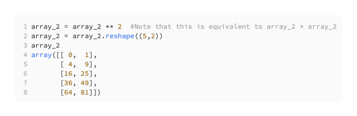
Ten elements make up the array. By calling the reshape method, you can reshape the array:
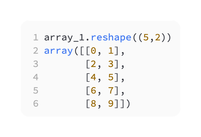
A three-dimensional NumPy array looks like a list of lists of lists (a five x two array looks like a list of lists of lists). It appears that you did not save the changes. After reshaping the array, save it as follows:
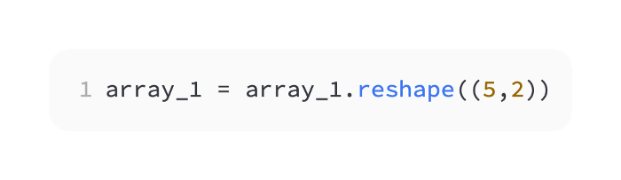
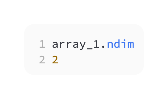
It is important to note that array_1 has become two-dimensional. In this case, it makes sense, since its shape is a list of lists and has two numbers:
Broadcasting with NumPy
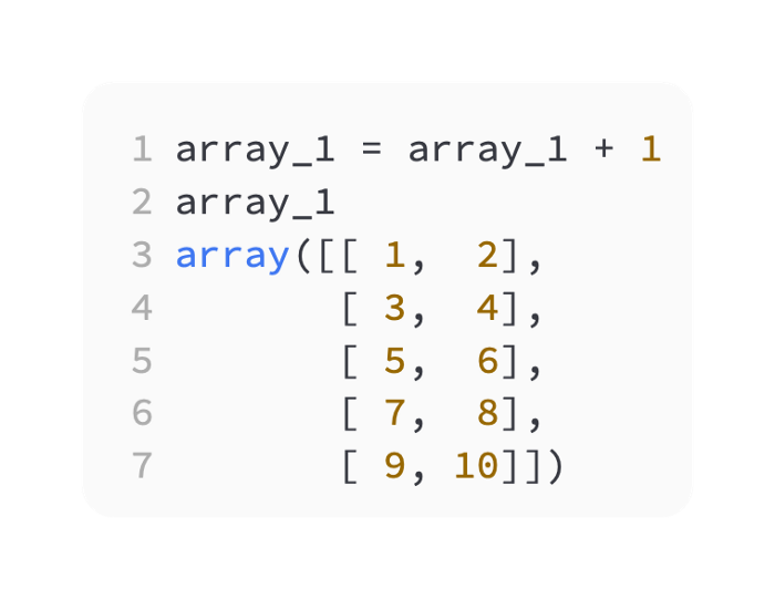
By broadcasting, add 1 to every element of the array. It is important to note that array changes are not saved:
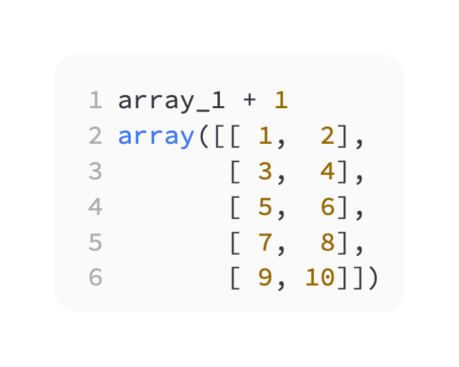
Broadcasting refers to stretching or broadcasting the smaller array across the larger array. This example adds the scalar 1 to array_1 after stretching it to a 5x2 shape.
Create a new array called array_2. The following results occur when you multiply an array by itself (this isn’t matrix multiplication; it’s array-wise multiplication):
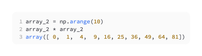
There has been a square root applied to every element. Multiplication has been performed element-by-element here. An example with more complexity is as follows:
Array_1 should also be changed:
Simply place a plus sign between array_1 and array_2 to add them element-by-element:
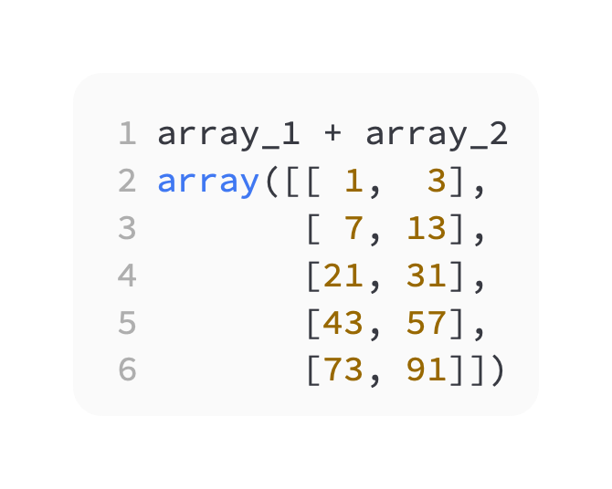
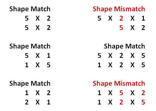
In formal broadcasting, all the numbers must either match or be one when comparing right to left the shapes of both arrays. From right to left, 5 X 2 and 5 X 2 are the same shapes. Despite this, the shape 5 X 2 X 1 does not match 5 X 2, since the second value from the right, 2 and 5, are mismatched:
Dtypes and arrays in NumPy are initialized
Besides np.arange, NumPy arrays can be initialized in several ways:
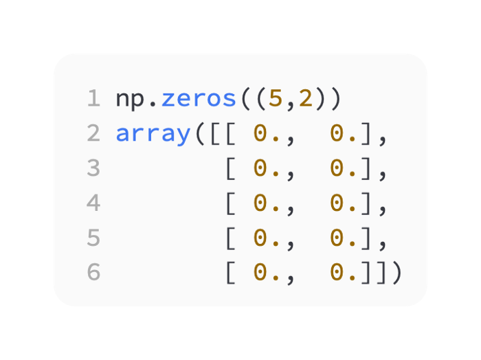
Using np.zeros, initialize a zero array. Zeros are created by the command np.zeros((5,2)):
A one-based array is created with np.ones. Make sure the ones are NumPy integer types by setting the dtype argument to np.int. It is important to note that scikit-learn expects np.float arguments in arrays. NumPy array elements are typed by their dtype. Throughout the array, it remains the same. There is an np.int integer type for every element in the array below.

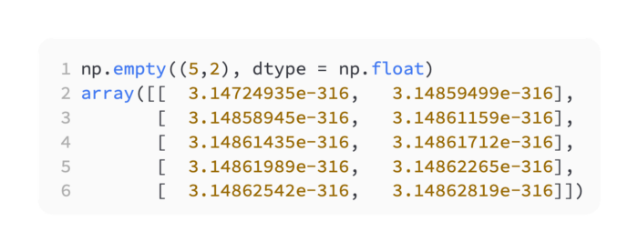
Using np.empty, you can allocate memory for an array with a specific size and dtype, but without any initial values:
Use np.zero, np.one, and np.empty to allocate memory for NumPy arrays with different start values.
Indexing
Find the two-dimensional array values using indexing:
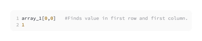
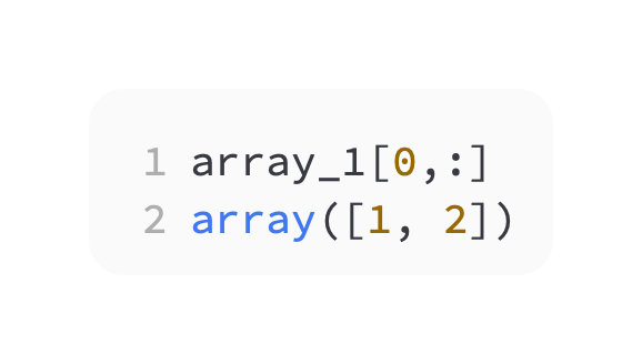
Take a look at the first row:
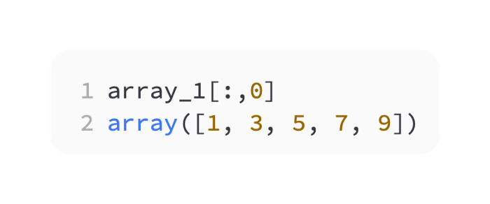
Look at the first column:
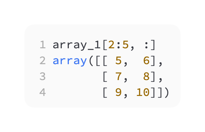
Values can be viewed along both axes. Take a look at the second through fourth rows as well:
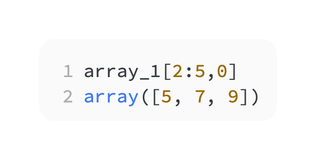
Along the first column, view only the second through fourth rows:
Boolean arrays
A Boolean indexing system is also available in NumPy:
The first step is to create a Boolean array:
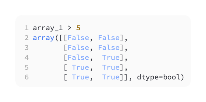
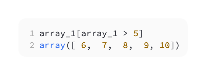
To filter by the Boolean array, place brackets around it:
Arithmetic operations
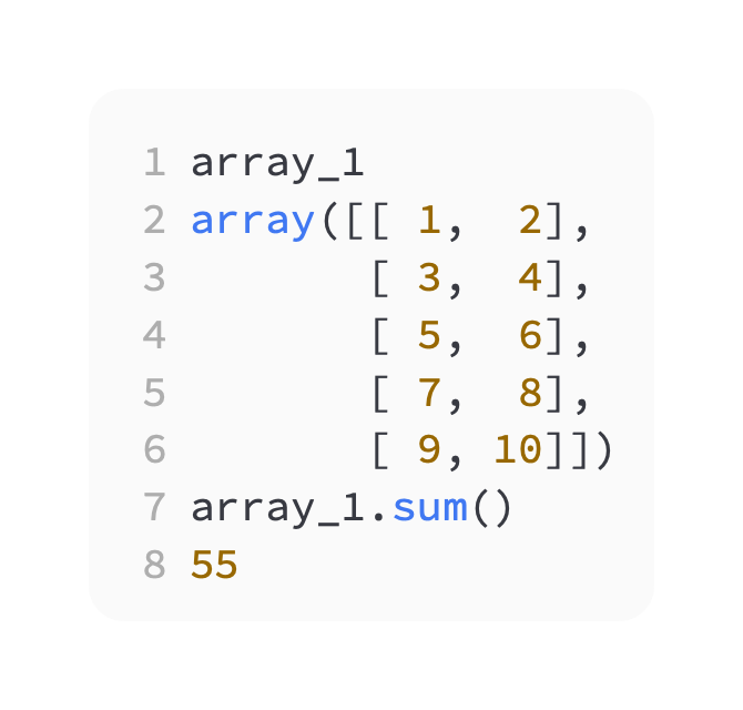
Using the sum method, add all the elements of the array. Here is array_1 again:
To find all the sums by row, follow these steps:
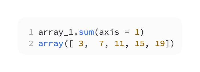
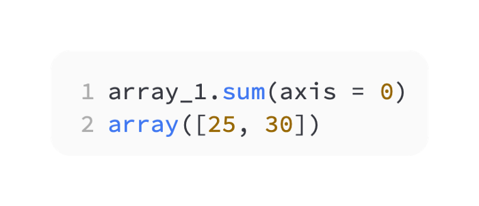
To find all the sums by column, follow these steps:
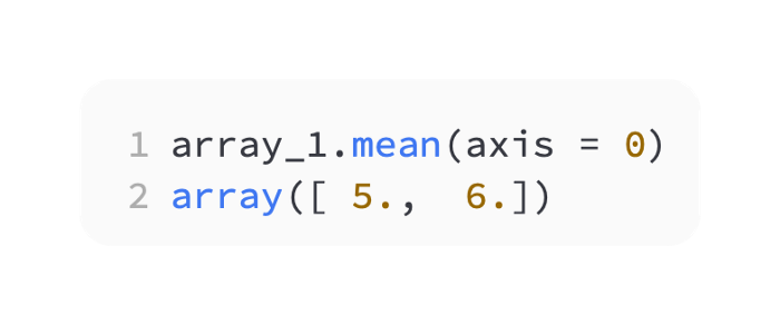
In a similar manner, find the mean of each column. There is a dtype of np.float on the array of averages:
NaN values
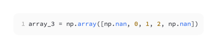
np.nan values will not be accepted by Scikit-learn. Consider array_3 as follows:
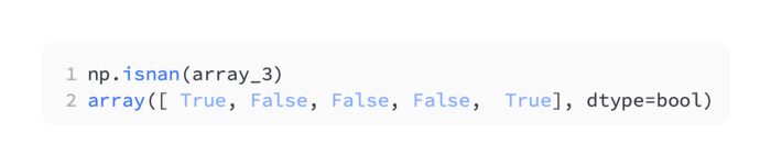
The np.isnan function creates a special Boolean array to find NaN values:
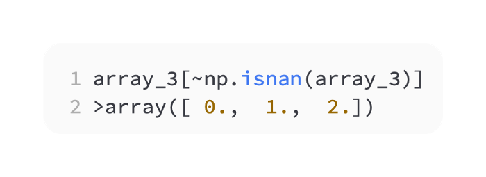
Negate the Boolean array and place brackets around it to filter out NaN values:
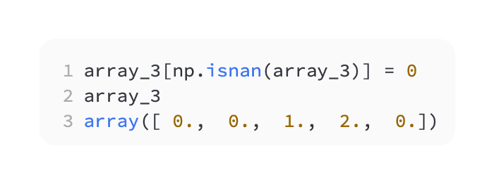
If you want to set the NaN values to zero, you can do so as follows:
As a matter of fact, NumPy is excellent at handling 2D tables of numbers. If you forget the NumPy syntax specifics, keep this in mind. NumPy arrays of real numbers must have no np.nan values missing to be accepted by Scikit-learn.
I have found that it is best to change np.nan to some value rather than tossing away data. The more I can keep track of Boolean masks and keep the data shape similar, the fewer coding errors I make and the more flexibility I have with my code.
Loading the iris dataset
The first step in machine learning with scikit-learn is to gather some data. With scikit-learn, we can load a variety of datasets, including the iris dataset.
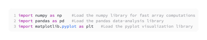
There are several imports in a scikit-learn program. Numpy, pandas, and pyplot libraries should be loaded within Python, preferably in Jupyter Notebook:
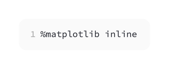
You can see an instant graphical output by typing the following in a Jupyter Notebook:
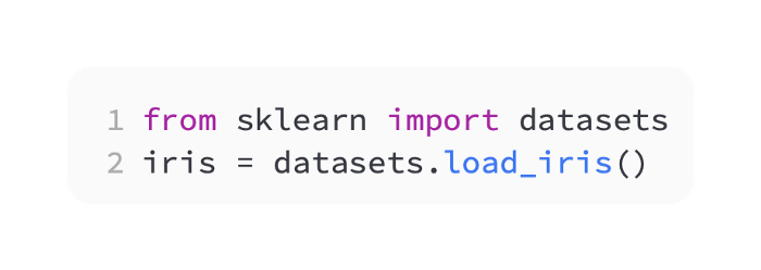
The iris dataset can be accessed from the scikit-learn datasets module as follows:
The diabetes dataset could have been imported similarly:
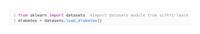
That’s it! A datasets module function load_diabetes() was used to load diabetes. The datasets available can be checked by typing:
datasets.load_*?After you try datasets.load_digits, you will find the dataset datasets.load_digits. As with any other loading function, you can access it with load_digits():
digits = datasets.load_digits()The dataset’s description can be found by typing digits.DESCR.
Viewing the iris dataset
Now that the dataset has been loaded, let’s take a look at what it contains. A supervised classification problem is posed by the iris dataset.
The observation variables can be accessed by typing:
Iris.dataAn array of NumPy values is output by this function:
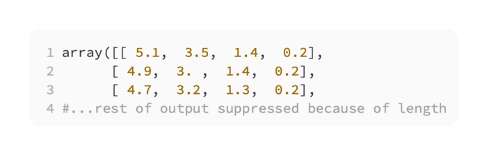
Using NumPy, let’s examine the array:
Iris.data.shapeThe following results are returned:
(150L, 4L)As a result, there are 150 rows by 4 columns of data. Take a look at the first row:
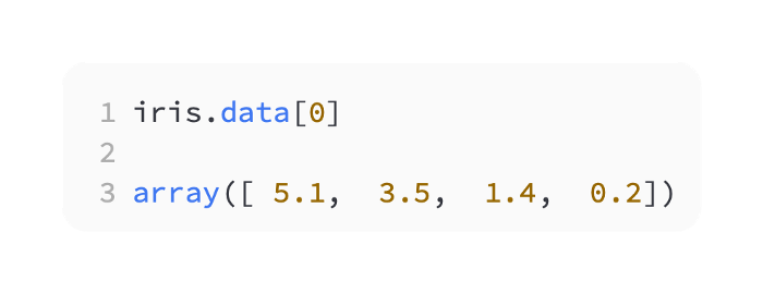
In the first row of the NumPy array, there are four numbers.
You can determine their meaning by typing:
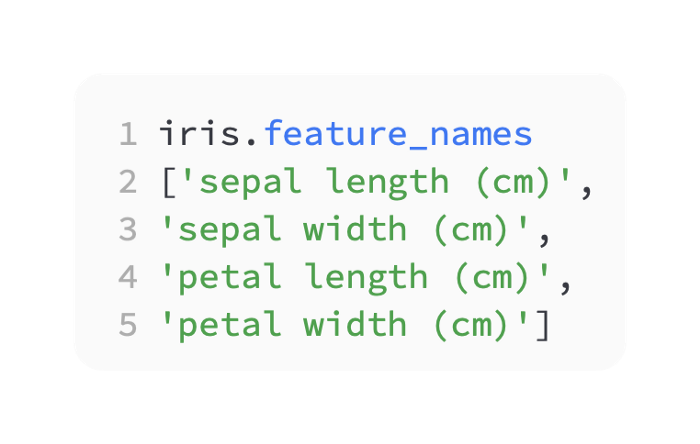
The names of the features or columns identify the data. It is a string that represents dimensions in different types of flowers. In total, 150 flowers were measured in centimeters for four measurements per flower. In the first flower, the sepal length is 5.1 cm, the sepal width is 3.5 cm, the petal length is 1.4 cm, and the petal width is 0.2 cm. In a similar manner, let’s examine the output variable:
Iris.targetAn array of three outputs is produced: 0, 1, and 2. An output can be selected from three options. Enter the following:
Iris.target.shapeAs a result, you get the following shape:
(150L,)There are 150 elements in this array (150 x 1). Here are the numbers that refer to:
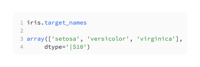
The output of the iris.target_names variable lists the English names for the numbers in iris.target. A setosa flower is number zero, a versicolor flower is number one, and a virginica flower is number two. Iris.target shows the following first row:
Iris.target[0]As a result, we end up with zero observations, which corresponds to the setosa flower in the first row.
Here’s how it works…
The data tables and two-dimensional arrays that correspond to examples are often used in machine learning. There are 150 observations of iris flowers of three types in the iris set. We would like to predict the type of flower based on new observations. Measurements in centimeters are made in this case. Real-world data is important to consider. I remember my high school physics teacher saying, “Don’t forget the units!”
Using the iris dataset, we aim to perform supervised machine learning by predicting a variable from observation variables based on a target array. Moreover, it is a classification problem, since we can predict three numbers based on the observations, one for each type of flower. We are trying to distinguish between categories in a classification problem. Binary classification is the simplest case. Multiclass classification is required for the iris dataset, which has three flower types.
Using Pandas to view the iris dataset
The iris dataset will be viewed and visualized using the handy pandas data analysis library. If you use the language R’s dataframe, you may already be familiar with the notion o.
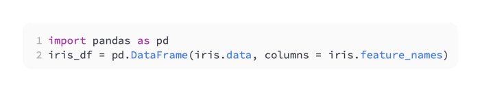
Using Pandas, a NumPy library built on top of the iris dataset, you can view the data as follows:
As arguments, create a dataframe with the observation variables iris.data, and columns names:
NumPy arrays are not as user-friendly as dataframes.
Analyze the dataframe for sepal length by looking at a quick histogram:
iris_df['sepal length (cm)'].hist(bins=30)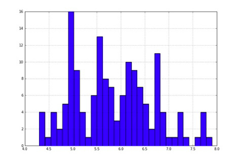
The target variable can also be used to color the histogram:
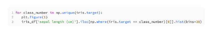
Draw a color histogram for each flower based on the target numbers. Here is a line to consider:
np.where(iris.target== class_number)[0]For each class of flower, the NumPy index location is found as follows:
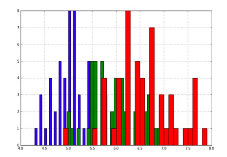
Histograms overlap, as can be seen in the figure below. The three histograms can therefore be modeled as three normal distributions. In machine learning, we can accomplish this if we model the training data as three normal distributions instead of the entire set. We then test the three normal distribution models we just created on the test set. The final step is to test whether our predictions were accurate on the test set.
Arrays of 2D NumPy columns and rows form the dataframe data object. Because of SQL’s long history, the fundamental data object in data science looks like a 2D table. As well as 3D arrays, NumPy also supports cubes, 4D arrays, and so forth. Also, these are frequently mentioned.
Matplotlib and NumPy plotting
NumPy’s matplotlib library makes it easy to visualize data with NumPy. Let’s quickly visualize some data.
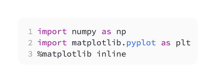
The first step is to import numpy and matplotlib. Using the %matplotlib inline command, you can view visualizations within an IPython Notebook:
Here is the main command in matplotlib, in pseudocode:
plt.plot(numpy array, numpy array of same length)By placing two NumPy arrays with the same length, you can plot a straight line:
plt.plot(np.arange(10), np.arange(10))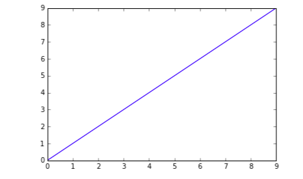
Exponents are plotted as follows:
plt.plot(np.arange(10), np.exp(np.arange(10)))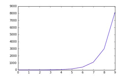
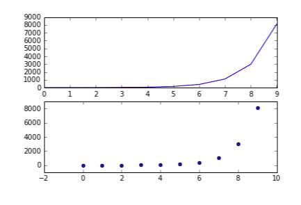
Put the two graphs side by side as follows:

In other words, from top to bottom:
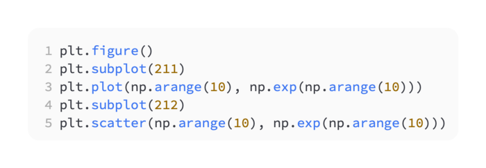
The first two numbers in the subplot command refer to the grid size in the figure instantiated by plt.figure(). The grid size referred to in plt.subplot(221) is 2 x 2, the first two digits. The last digit refers to traversing the grid in reading order: left to right and then up to down.
In a 2 x 2 grid, traverse the reading order one through four as follows:
