Making Profitable Trade Using Google Trends
Making Profitable Trade Using Google Trends
A paper published in Scientific Reports in 2009 was titled Quantifying Trading Behavior in Financial Markets Using Google Trends.

Based on the frequency of certain words in Google searches, is it possible to predict efficient trading strategies?
As part of the data collection and analysis process, the authors went through a number of interesting steps. To examine patterns of searches for financial information, they developed a set of financial keywords based on the Financial Times website.
They used Google Sets (now defunct) to build a robust set of keywords. Based upon changes in the search history for all of their terms, they defined a trading execution plan to buy or sell based on data collected from Google Trends. All the keywords were run through the strategies and each phrase’s investment value was ranked.
Can you tell me what their conclusion was? This appears to be a very good method of beating random investments in the S&P 500 index. There is some debate about this result, but the process itself is interesting. In this example, historical data are brought in from multiple sources, and then statistical analysis is used to determine whether a portfolio is worth investing in based on data from another source.
Our purpose in this article is to study their data and reproduce their results as closely as possible (and we will be very close to their results). Using pandas, we can easily reproduce all of their steps. Both of these examples illustrate how social data can be collected and used to make money. The authors also provide an interesting introduction to using pandas to develop trading strategies, which will be the focus of this article’s remaining sections.
Following are the topics we will discuss in detail:
This article describes how Google Trends can be used to quantify trading behavior in financial markets
Using Google Trends to retrieve trend data
Data from Quandl for Dow Jones Index
Ordering trades
Investing results calculation
Final thoughts
Setting up a notebook
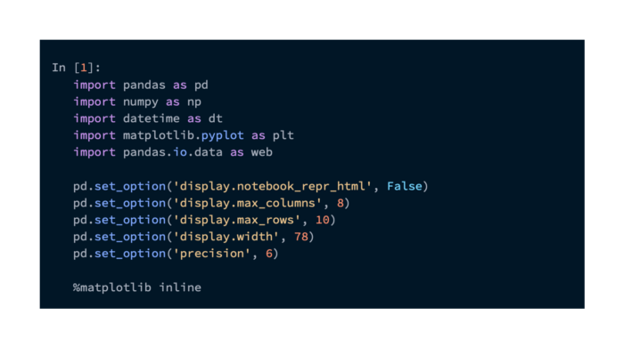
This code is needed for executing and formatting output in the workbook and examples. Several options for fitting data to the page in the text, as well as the CSV (comma-separated value) and RE (regular expression) frameworks are included, as with previous articles. I am referring to the following code:
Quantifying trading behavior in financial markets using Google Trends
Using the social habits of people seeking and gathering information as a basis for predicting market movements, the authors of this paper claim, financial markets are a prime target for analyzing market movements in order to gain a competitive advantage so that personal financial gains can be realized.
In addition, they investigate whether search query data from Google Trends can provide historical insight into how stock market traders gather information prior to making trading decisions.
For the period of 2004–01–01 to 2011–02–28, the authors collected data from Google Trends and the Dow Jones Industrial Average (DJIA). Financial terms (specifically the term debt) can result in a bias towards financial results when they are seeded into the process. Using Google Sets, they recommend additional search terms based on the seed terms based upon the initial set of terms. 98 different search terms are selected and trading decisions are made based on the volume of searches for each term.
A DJIA closing value is used on Monday or Tuesday depending on the weekday. Sunday through Saturday is the reporting interval for Google Trends data.
According to the authors, search terms in Google are correlated with DJIA movements in order to illustrate the relationship between search behavior and market movements. According to the authors, the stock market should rise if, after a three-week window, Google searches for a term have increased, followed by an upturn in the following week. The trader should, therefore, initiate a long position and transfer all current holdings into it. Considering the property’s predicted market gains, a profit will be made during that one week period as the investment’s value increases.
Our holdings should be sold short at the end of the first day of the next trading week if the number of searches decreased from the previous three-week average. During this period, we will profit if the market declines.
A performance analysis is also presented. Based on their strategy, their position increased for the search term “debt”. The solid blue line represents their production of 326 percent in the following graph:
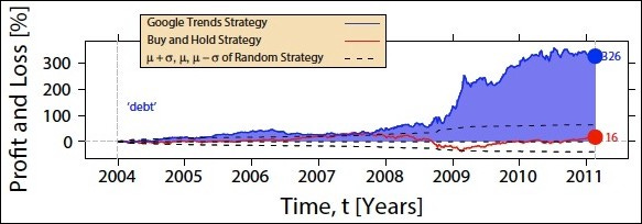
Based on the simulation of 10,000 realizations of the random strategy, the dashed lines represent the standard deviation of the cumulative return.
The authors conclude that the Google Trends strategy has a significantly larger difference in results than random strategies, proving that their assertion is valid.
Since their strategy involves only 104 transactions a year, they neglect transaction fees, stating that they could affect the results if considered. Their goal was to determine the overall effectiveness of relating social data to market movement to gain a competitive edge. They ignored transaction fees.
Using Google Trends data and DJIA data, we will establish a model for replicating this strategy by evaluating search terms for “debt” for the same period as in the paper. Rather than validating their research, we aim to learn various concepts and how to implement them in Python with Pandas. In this course, you will learn how to obtain data from disparate sources, model a trading strategy, and evaluate the effectiveness of a trading strategy using a trading back-tester.
Collection of data
In this study, we will create a DataFrame containing both DJIA and Google Trends data provided by the authors, along with dynamically collected web data for each. Our data will be compared to what they collected, and then we will use their algorithm to simulate trades.
The study used data available on the Internet. The text includes it as an example. This information will also be collected dynamically using pandas to demonstrate those processes. Both the authors’ and our newly collected data will be used for the analysis.
We may also encounter snags in data collection, but this is not uncommon in the real world. The DataReader class of pandas no longer supports DJIA data, so we can’t fetch it with Yahoo! A web-based service called Quandl will be used to overcome Yahoo! Finance’s lack of DJIA data also a good introduction to a reader.
Second, Google Sets, which the authors used to generate their search terms, has been deactivated by Google. Unfortunately, that’s not what the authors claim to have the best results with, so we’ll model the results based on “debt”.
In addition, Google Trends data is difficult to access. Our data will be dynamically downloaded from a .csv file that I will provide.
The data from the paper
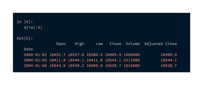
There are online copies of the data from the paper, but I have also included them in the code samples as well. Using the following command, it can be loaded into Pandas:
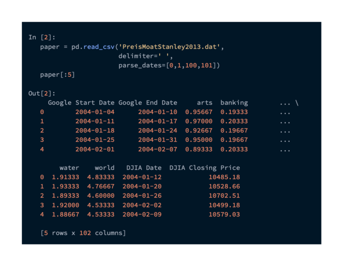
A single file containing all DJIA data combined with a normalization of search volumes was used in the paper to generate the data. In a search, each keyword is represented by a column.
To extract the DJIA closing price and date for each row, we need to extract the debt values, the Google Trends Week End date, and the Google Trends Week End date. Here is the pandas code we need to do this:
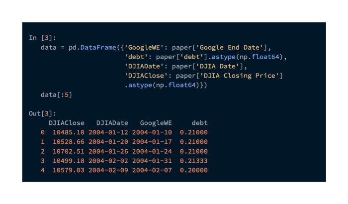
Data from Google Trends was normalized relative to all searches generated by the paper. When we get this data on our own, we will be able to see the raw values. Data like this doesn’t matter for its value, but for how it changes over time, which can be used to indicate relative changes in search volumes.
Using Quandl to gather our own DJIA data
DJIA data could be retrieved using the pandas DataReader class from Yahoo! Finance in the past. Due to Yahoo!’s discontinuation of DJIA data, we need a replacement. The data can be retrieved from Quandl (http://www.quandl.com/). Quantitative analysis datasets are provided by Quandl. Their API provides API-based access to their data, and accounts can be created for free. Additionally, they provide Python, Java, and C# client libraries. We will use this command in this discussion:
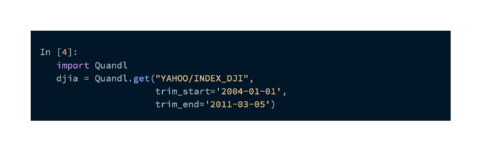
The code packet for the text includes a file that contains this data:
The following command displays the retrieved data. During the specified dates, it shows the following daily DJIA variables:
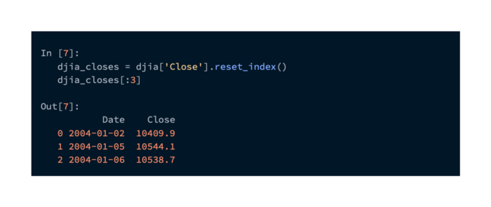
This data contains Close values that we would like to merge into our DataFrame. The DJIADate column will provide us with the data we need to align our dates. Additionally, we would like to drop all days with data that is not aligned. Using pandas merge, we can accomplish this easily. It is necessary to extract the Close values from the index and move them to a column to perform this operation:
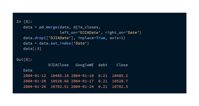
Using the DJIADate and Date columns from the two DataFrame objects, we will create a new DataFrame object with the two datasets merged (we do away with DJIADate as it is redundant, and set Date as the index) as follows:
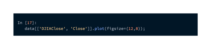
Based on this data, it appears that the DJIA closing prices are fairly well matched. Both series are practically identical when plotted next to each other. Data can be plotted using the following command:
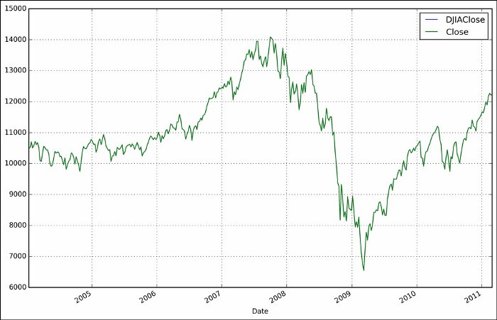
Statistical differences between the values can also be checked, as shown below:
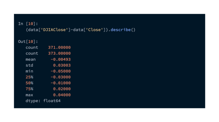
It appears that the overall differences are well under a tenth of a point and are most likely the result of rounding errors.
The two series of data can be examined for correlation one last time:
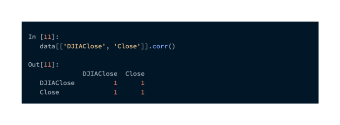
The correlation is perfect. By summarizing our data this way, we can be confident that it has been prepared correctly.
Statistics from Google Trends
Google Trends data for the term “debt” was provided by the authors. This is convenient, but we would like our own Google Trends data. It appears that API access to this data is not available at this time. However, we have a few options for retrieving it. Automating a web crawl can be achieved using the mechanized framework. Alternatively, we can download the CSV data we need using the web portal.
http://www.google.com/trends/ lets you search for any term and get trend data associated with that term. Searching for the term debt results in the following command:
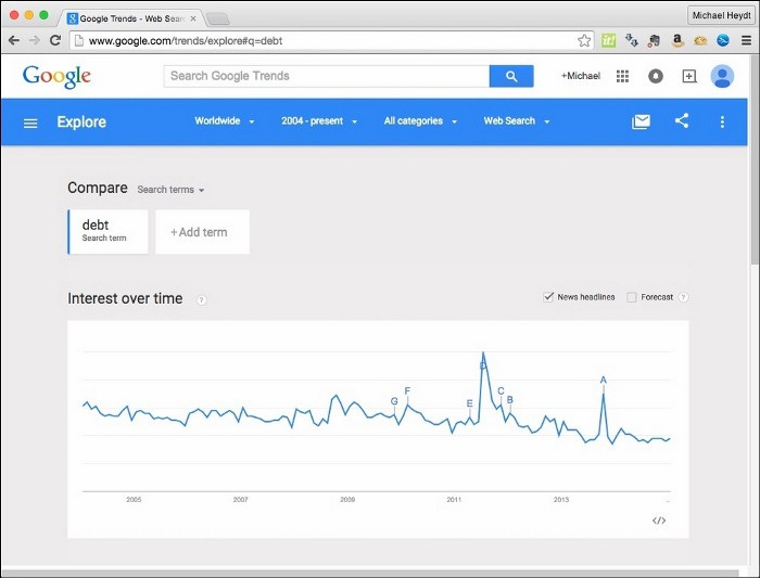
We can’t use this in our Pandas application because it’s too pretty. The following screenshot shows that, if we click on the options button, we can download the data as a CSV file:
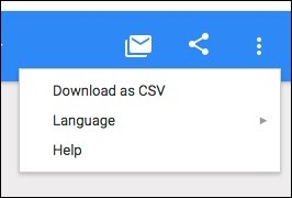
Here is a link for you to download. A data folder for the samples is also provided. Trends_report_debt.csv is the file name. A few lines of the file are shown in the following command:
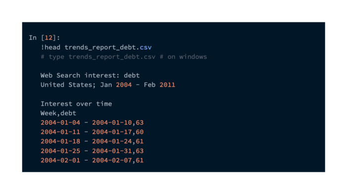
Getting the data from this CSV file requires some processing. Reading the file and selecting trend data for the range of dates we are working with is done with the following command:
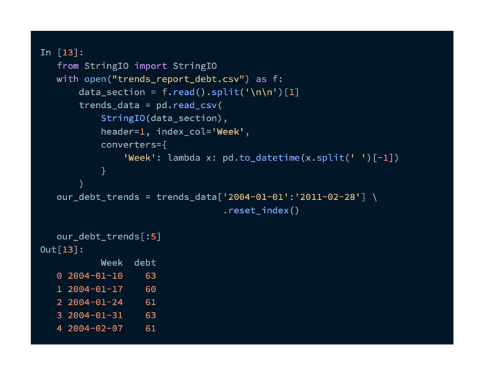
Searches are not counted by these numbers. To get a sense of how the volume changes over time, you can compare it with the other periods in the dataset provided by Google. It’s unfortunate that they keep the good data to themselves, but we can still use this information.
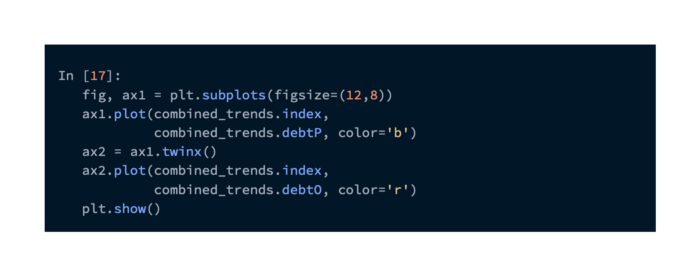
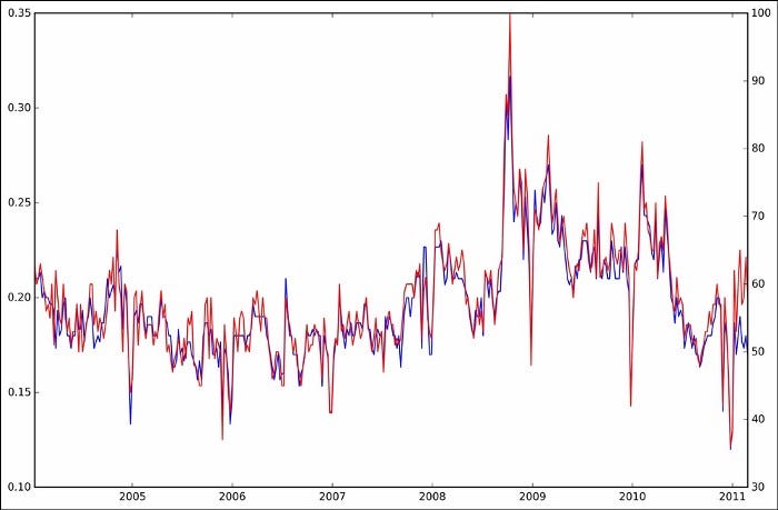
As a first step, we can combine these data into our dataset and check their conformance. The same procedure will be followed and pd.merge() will be used again. On the left, we’ll join the GoogleWE column and on the right, the Week column. Merging, renaming debt columns, and moving indexes can be accomplished with the following command:

To check how closely our trend data correlates with the trends used in the paper, we can create a new DataFrame with the normalized trend data from both papers (indexed by GoogleWE):
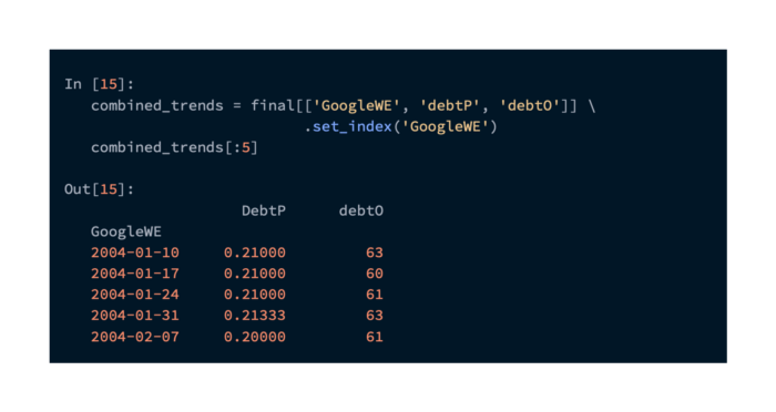
These series are highly correlated based on correlation analysis. Due to the constant renormalization of the data retrieved from Google, the trend data that was captured earlier will differ slightly:
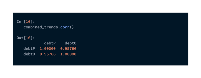
Taking a look at the correlation between these two, we can see that they are very closely related: