Master Naive Bayes For ML
From labelled training data, we learned algorithms for regression and classification using supervised learning tasks.

Our first unsupervised learning task will be described in this article: clustering. Cluster analysis is used to identify groups of similar observations within unlabeled data. Using an image compression problem as an example, we will discuss the K-means clustering algorithm. We will finally examine a semi-supervised learning problem that incorporates clustering and classification.
Clustering
Unsupervised learning is focused on discovering hidden patterns or structures in unlabeled training data as described in the previous article, The Fundamentals of Machine Learning. In clustering or cluster analysis, observations are grouped so that those within a group, or cluster, have a greater degree of similarity to those within another group. We will represent observations as n-dimensional vectors, just as with supervised learning.
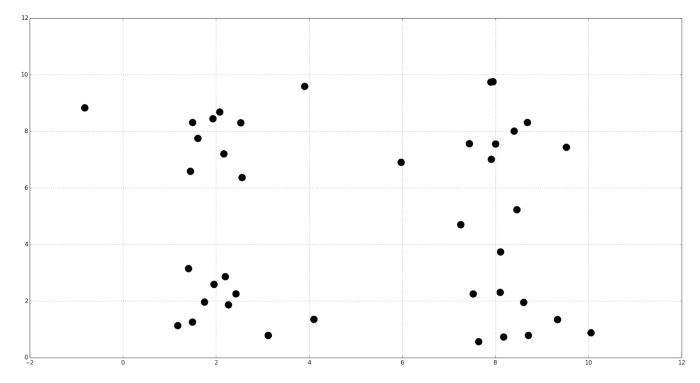
Assume, for example, your training data consist of the following samples:
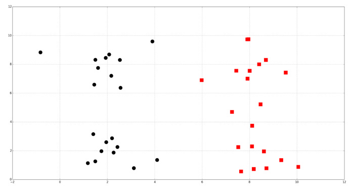
Squares and circles indicate two groups that may be formed by clustering:
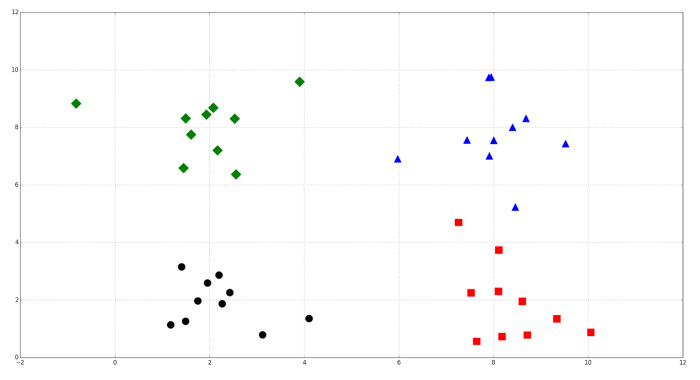
It is also possible to cluster into four groups as a result of clustering:
Exploring a dataset using clustering is a common practice. Network clustering can be used to identify missing connections between people and to identify communities. Gene expression patterns are grouped together using clustering in biology. Clustering is sometimes used in recommendation systems to identify products or media users might be interested in. Consumer segments can be found using clustering in marketing. We will demonstrate how to cluster a dataset using K-means in the following sections.
K-means
Known for its scalability and speed, the K-means algorithm is a popular clustering algorithm. K-means involves redistributing instances among clusters with the closest centroids by moving cluster centers to their average positions and reassigning them to the cluster with the closest centroids. K-means automatically assigns observations to clusters, but cannot determine the appropriate number of clusters. It uses a hyperparameter called k to specify the number of clusters to create. A positive integer less than k must be used as a training set’s k. The clustering problem’s context may specify how many clusters to use. A shoe manufacturer, for example, may know that it can produce three new models at a time. By surveying customers and creating three clusters based on the results, it learns what groups of customers to target with each model. The optimal number of clusters may not be determinable for all problems, and some problems may not require a specific number of clusters at all. As we discuss later in this article, the elbow method is a heuristic for estimating the optimal number of clusters.
For K-means, the parameters are the centroids of the clusters and the observations assigned to each cluster. The optimal values of K-means’ parameters are found by minimizing a cost function, just like those of generalized linear models and decision trees. According to the following equation, K-means has the following cost function:
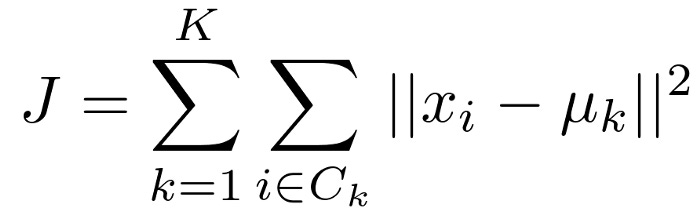
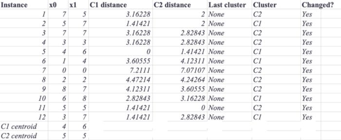
Here, μk is the centroid of cluster k. The distortions of the clusters are summed in the cost function. The distortion of each cluster can be calculated by adding the squared distance between its centroid and its constituent instances. Clusters with compact instances exhibit small distortion, while clusters with scattered instances exhibit large distortion. Observations are assigned to clusters and then the clusters are moved iteratively to learn the parameters that minimize the cost function. It is often necessary to select instances at random to initialize cluster centroids. During each iteration, K-means assigns observations to the closest cluster and then moves the centroids to the mean location of the observations. Using the training data shown in the following table, let’s work through an example by hand:
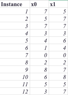
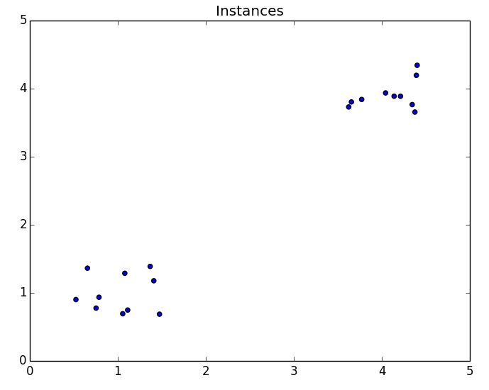
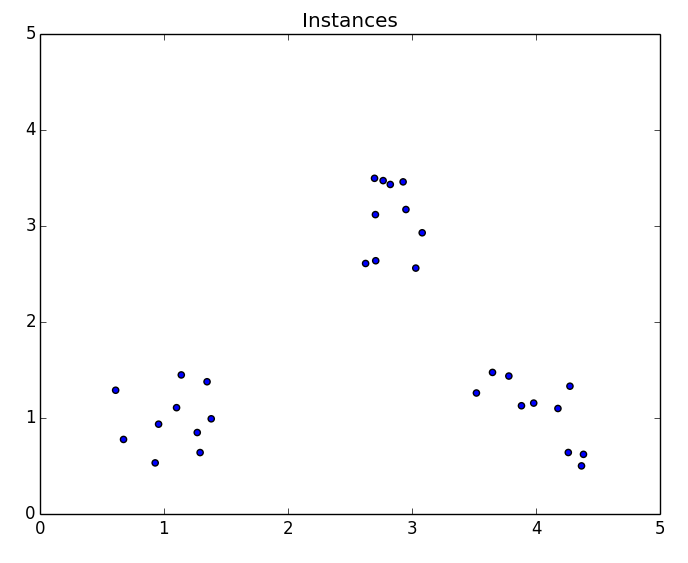
Two explanatory variables are used, each with one feature extracted. The following figure shows the instances:
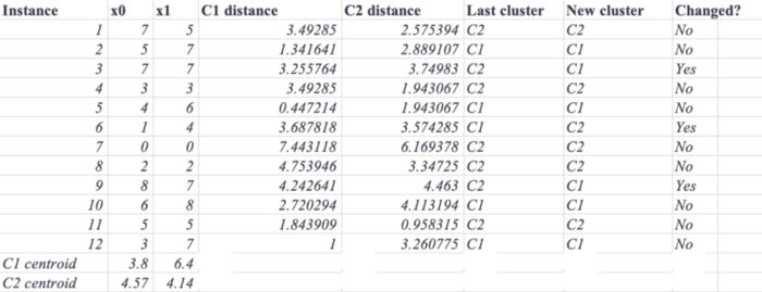
If K-means initializes the centroid to the fifth instance for the first cluster, and to the eleventh instance for the second cluster, the results will be as follows. Each instance will be assigned to the cluster with the closest centroid based on its distance from both centroids. In the following table, the Cluster column shows the initial assignments:
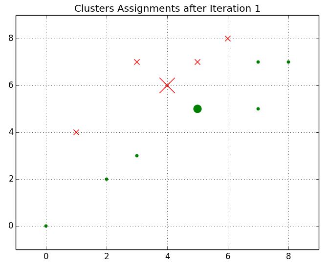
A graph showing the centroids plotted and initial cluster assignments can be found below. A cluster has instances marked with an X, whereas a cluster has instances marked with dots. There is a larger difference between the marker size for the centroids and the marker size for the instances.
After recalculating the distances between training instances and centroids and reassigning the instances to the closest centroids, we will move both centroids to the means of the instances they represent. In the following graph, you can see the new clusters. Several instances have changed their assignments and the centroids are diverging.
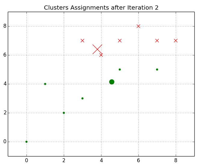
Based on the second iteration of the algorithm, the following plot shows the centroids and cluster assignments:
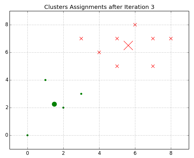
Instances will be reassigned to their nearest centroids after the centroids are moved to the means of the locations of their constituents. Here is a figure showing the centroids diverging:
As long as k-means does not find a stopping criteria for iteration, the instances’ centroid assignments will remain the same in the next iteration. Normally, this threshold represents either the difference between the cost function values for subsequent iterations, or the change in the centroids’ positions between successive iterations. A k-means algorithm will converge on an optimal solution if these stopping criteria are small enough.
It is worth noting, however, that as the stopping criteria decrease, the time required to converge increases. Also, regardless of the stopping criteria, K-means will not necessarily converge to the global optimum.
Local optima
The centroids of K-means are usually initialized to random positions. In some cases, this random initialization leads to K-means converge to a local optimum because the centroids are set in unlucky positions. The following positions are assumed for two cluster centroids by K-means:
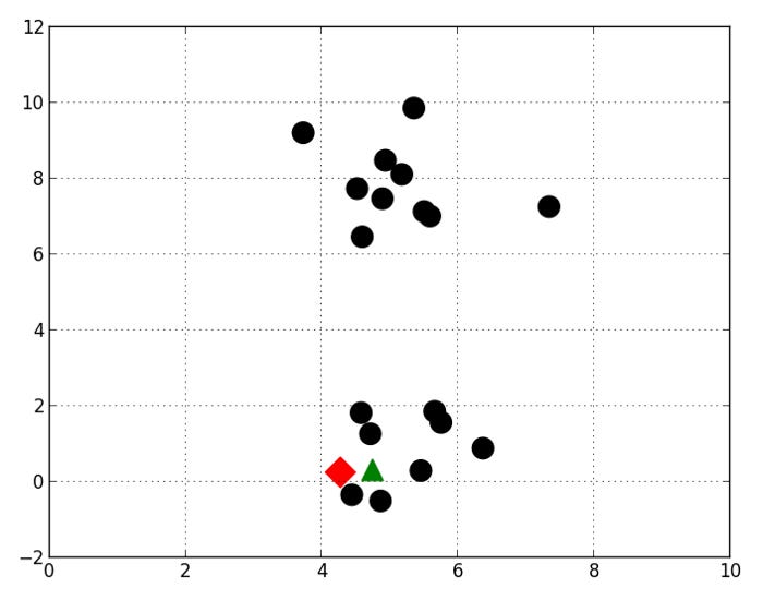
This figure illustrates how K-means eventually converge on a local optimum. The top and bottom clusters of observations may be more informative, but the middle clusters are more likely to be informative. Local optima vary in quality. Several hundred or dozens of K-means are usually repeated to avoid unlucky initialization. Randomly initializing the cluster positions is done in each iteration. The best initialization is chosen based on its ability to minimize the cost function.
The elbow method for selecting K
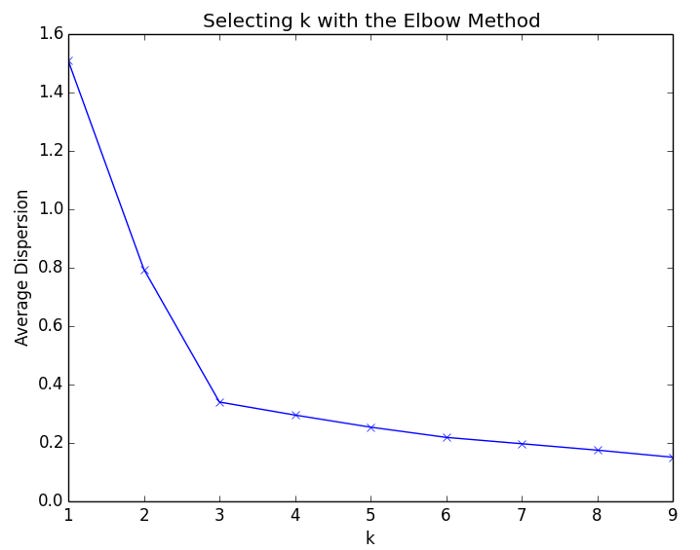
The elbow method can be used to estimate the optimal number of clusters if k is not specified by the context of the problem. In the elbow method, the cost function is plotted based on the values of k. For each cluster, the average distortion decreases as k increases, and the instances are closer to their centroids as k increases. Increasing k, however, will result in a declining improvement in average dispersion. It is called the elbow when the improvement to dispersion declines most at a given value of k. In this example, we will use the elbow method to determine how many clusters to create. Based on the scatter plot below, we can see that there are two obvious clusters in the data:
This code calculates and plots the mean cluster dispersion for each value of k from 1 to 10:
As a result of the script, the following plot is generated.
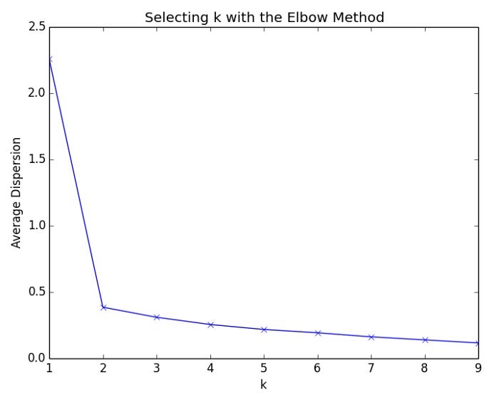
As k increases from 1 to 2, the average dispersion improves rapidly. For values of k greater than 2, there is little improvement. In this example, we will apply the elbow method to a dataset with three clusters:
Here is a plot of the elbows for the dataset. Adding a fourth cluster results in the greatest decline in the rate of improvement to the average distortion. Therefore, k should be set to 3 for this dataset based on the elbow method.
Evaluating clusters
A machine learning system learns from experience and improves its performance as measured by some metric through experimentation. K-means is an unsupervised learning algorithm that does not require labels or ground truth for comparison. Nevertheless, intrinsic measures can be used to evaluate the algorithm’s performance. The distortions of clusters have already been discussed. The silhouette coefficient is another measure of clustering performance. An indicator of compactness and separation between clusters is the silhouette coefficient. Increasing quality yields larger clusters; small, overlapping clusters yield small clusters; compact clusters yield large clusters. In a set of instances, the silhouette coefficient is calculated by averaging the scores of the individual samples. This equation calculates the silhouette coefficient for an instance:
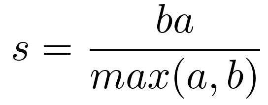
Cluster instances are separated by a mean distance called a. This distance is measured between the instance and the next closest cluster instance. For each of the four runs of K-means, the silhouette coefficient is calculated for two, three, four, and eight clusters from the toy dataset:
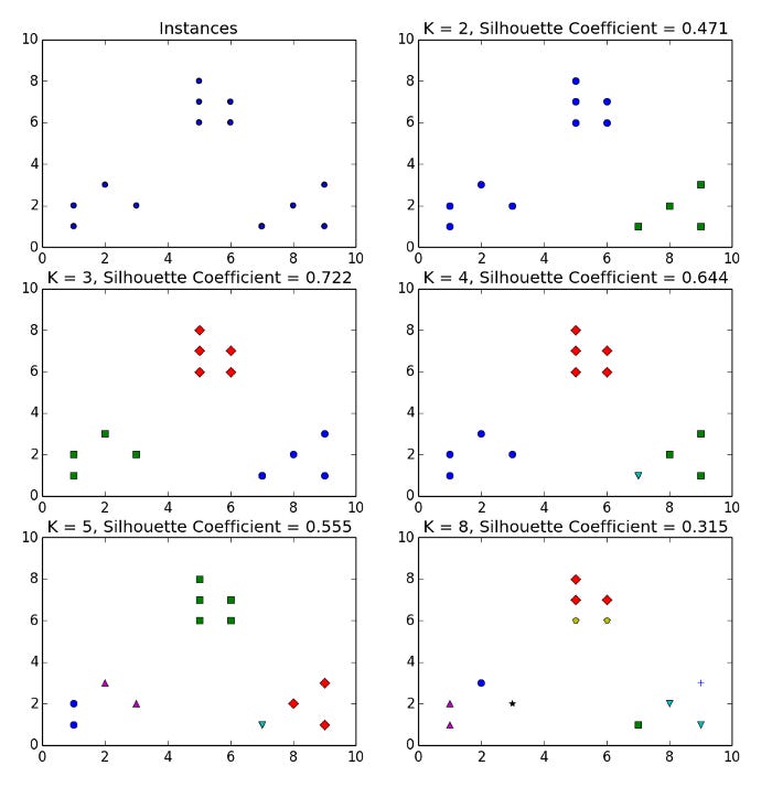
Three obvious clusters can be seen in the dataset. In this case, K equals 3 gives the greatest silhouette coefficient. With K = 8, clusters of instances share the same closeness as clusters in some of the other clusters, and their silhouette coefficient is the smallest.
Image quantization
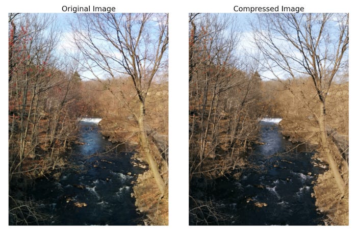
In previous sections, we explored dataset structure using clustering. Now let’s apply it to another problem. Image quantization is a method for reducing the number of colors in an image by replacing a range of similar colors with one color. Because fewer bits are required to represent colors, quantizing reduces the size of the image file. This example illustrates how clustering can be used to discover an image’s most important colors using a compressed palette. The compressed palette will then be used to rebuild the image.
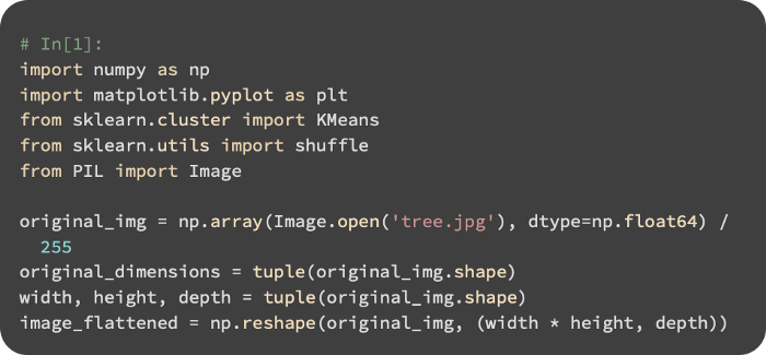
We begin by reading the image and flattening it:
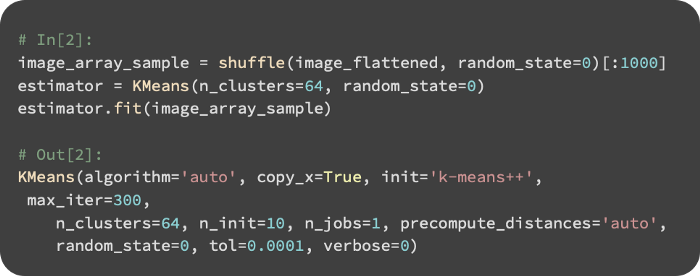
From 1000 randomly selected colors, K-means is used to create 64 clusters. The compressed palette will be divided into clusters of colors:
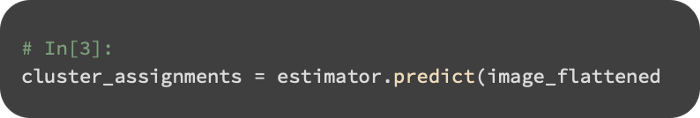
Using the original image, we predict cluster assignments for each pixel:
After creating the compressed palette and cluster assignments, we create the compressed image:
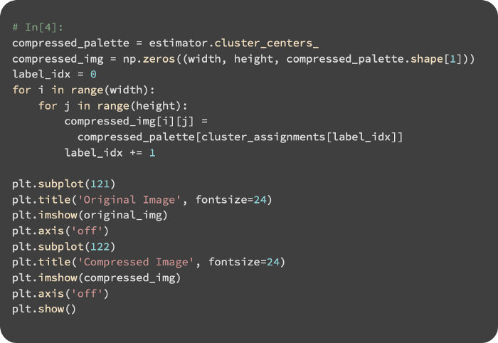
Below is a comparison of the original and compressed images: