Master Neural Network Algorithms
The importance of Artificial Neural Networks (ANNs) has been attributed to a combination of factors.
Due to the growing complexity of problems, the explosion of data, and the availability of inexpensive computing clusters, there is a growing need for complex algorithms.
Most major advances in leading-edge tech fields like robotics, natural language processing, and self-driving cars have emerged from this research area, which is rapidly evolving.
An ANN is composed of neurons, which are its basic unit. By organizing multiple neurons in a layered architecture, the ANN uses the power of multiple neurons efficiently. Neurons are chained together in layers in an ANN to create a layered architecture. In each of these layers, a signal is processed differently until the final output is generated. We will learn in this article how ANNs’ hidden layers enable deep learning, which is widely used in applications such as Amazon’s Alexa, Google’s image search, and Google Photos.
First, a typical neural network is introduced and its main components are discussed. After that, it discusses the various types of neural networks and the activation functions used in these neural networks. Following that, we discuss the most widely used neural network training algorithm, backpropagation. Following that, the transfer learning technique is explained, which simplifies and partially automates model training. Lastly, a real-world example application is used to demonstrate how deep learning can be used to flag fraudulent documents.
This article discusses the following concepts:
An understanding of ANNs
Evolution of artificial neural networks
The training of a neural network
A framework and toolset
The transfer of learning
Fraud detection using deep learning: a case study
The basics of ANNs should be reviewed first.
ANNs: An overview
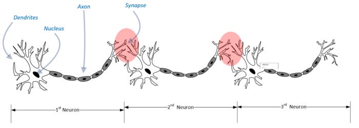
In 1957, Frank Rosenblatt proposed the concept of neural networks based on the functioning of neurons in the human brain. It is helpful to briefly examine the layered structure of neurons in the human brain in order to fully understand the architecture. To understand how neurons are chained together in the human brain, look at the following diagram.
The dendrites of the human brain act as sensors that detect signals. Nerve cells transmit signals to their axons, which are long and slender projections. This signal is transmitted by the axon to muscles, glands, and other neurons. Signals are transmitted from neurons to other neurons through interconnected tissue called a synapse. Through this organic pipeline, the signal travels until it reaches the target muscle or gland, where it causes the desired effect. When a signal passes through a chain of neurons and reaches its destination, it typically takes seven to eight milliseconds:
In order to solve a complex mathematical problem, Frank Rosenblatt developed a technique inspired by this natural architectural masterpiece of signal processing. It looked like a linear regression model when he first attempted to design a neural network. There were no hidden layers in this simple neural network, so it was called a perceptron. Here is a diagram that illustrates what I mean:
Let’s try to represent this perceptron mathematically. On the left side of the diagram are the input signals. The inputs (x1, x2, ..xn) are weighted by their corresponding weights (w1, ..wn) before being summed:
It is a binary classifier since this perceptron’s output depends on the aggregator’s output (shown as ∑ in the diagram). At least one of the input signals must be valid in order for the aggregator to produce a true signal.
The evolution of neural networks over time is now the subject of our discussion.
Neural network training
The process of training a neural network involves using a dataset. Here is an overview of what a typical neural network looks like. To train a neural network, we calculate the optimal weights for the network. In training, examples are used as training data to iteratively build the model. There are examples in the training data for different combinations of input values that show the expected output values.
A Neural Network’s Anatomy
A neural network consists of the following components:
Neural networks are composed of layers. Every layer is a data-processing module that filters data. An input is processed in a certain way, followed by an output. Each layer processes data and shows patterns relevant to the business question we are trying to answer.
Loss function: Loss functions provide feedback signals for learning iterations. Loss functions provide deviations for individual examples.
A cost function represents the loss function over a complete set of examples.
Loss function feedback signal is interpreted by an optimizer.
Data inputs: Data inputs are used for training neural networks. Variables are specified here.
In order to calculate the weights, the network must be trained. Each input is assigned a weight based on its importance. During training, a particular input is given a greater weight value if it is more significant than other inputs. The large weight value (that acts as a multiplier) will strengthen even a weak signal for that important input. Each input is turned according to its importance by weight.
Activation function: Multiplying values by weights, then aggregating. Based on the type of activation function chosen, how they are aggregated and interpreted will vary.
Now let’s consider one of the most important aspects of neural network training.
We take each example one at a time while training neural networks. Using our under-training model, we generate the output for each example. Using the expected output and predicted output, we calculate the difference. This difference is called the loss for each individual example.
Losses over the entire training dataset are referred to as cost. In order to find the smallest loss value, we keep training the model until the weights are found. We adjust the weight values throughout the training process until the set of weights results in the lowest possible overall cost. The model is trained once it reaches the minimum cost.
Gradient Descent Defining
In neural networks, training is the process of finding weight values that work. When we train a neural network, we start with default or random weight values. Our predictions are then improved by iteratively changing the weights using an optimizer algorithm, such as gradient descent.
When we iterate through a gradient descent algorithm, we start with random values of weights to optimize. Iteratively, the algorithm changes the weights in such a way that the cost is minimized in each iteration.
An explanation of the gradient descent algorithm is provided in the following diagram:
The input vector X is shown in the preceding diagram. Target variable Y actually has value Y, while target variable Y’ has predicted value Y. Based on the actual value, we determine the deviation from the predicted value. Once the weights have been updated, we repeat the steps until the cost has been minimized.
There are two factors that will determine how the weight is varied in each iteration of the algorithm:
Getting the minimum of the loss function requires a certain direction
A learning rate is a measure of how much change should be made in the chosen direction
The following diagram illustrates an iterative process:
The diagram shows how gradient descent finds the minimum cost by varying the weights. We will explore the next point on the graph based on our learning rate and direction.
The learning rate should be selected carefully. A problem that takes a long time to converge may be due to a small learning rate. A problem will not converge if the learning rate is too high. We can observe that the dot corresponding to the current solution oscillates between the two opposite lines in the preceding diagram.
The next step is to minimize a gradient. X and Y are the only variables to consider. In order to calculate the gradient of x and y, follow these steps:
A method for minimizing gradients is as follows:
As well as finding optimal or near-optimal weights for a neural network, this algorithm can also find optimal or near-optimal parameter values.
In the network, gradient descent is calculated backwards. In order to reach the first layer, we calculate the gradient of the final layer first, then the second-to-last layer, and so on. In 1985, Hinton, Williams, and Rumelhart introduced a method called backpropagation.
Activation functions are next on the list.
The activation functions
Activation functions determine how the inputs to a particular neuron are processed.
An activation function determines how inputs are processed in a neural network, as shown in the following diagram:
As seen in the preceding diagram, activation functions generate results that are passed on to outputs. Activation functions determine how input values are to be interpreted in order to produce outputs.
It is possible to produce different outputs using different activation functions for exactly the same input values. Using neural networks to solve problems requires understanding how to select the right activation function.
Now let’s examine each activation function individually.
Function for determining thresholds
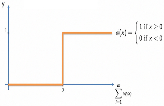
An activation function that is as simple as possible is the threshold function. Threshold functions produce binary outputs: 0 or 1. In the event that any input exceeds 1, 1 will be produced as the output. Following is a diagram that explains this:
When the weighted sums of the inputs show signs of life, the output (y) becomes 1. Thus, threshold activation functions are very sensitive. Due to glitches or some noise, it can be accidentally triggered by the tiniest signal.
The sigmoid
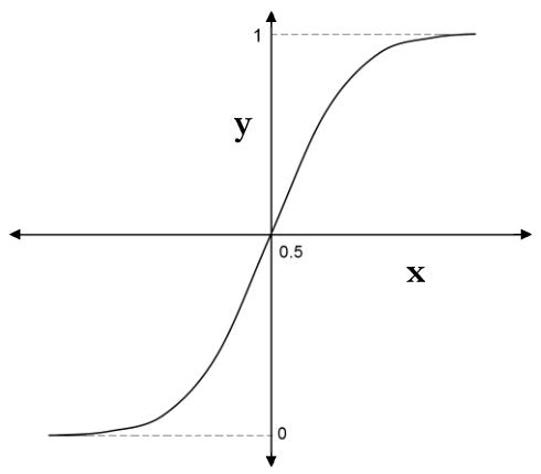
An improvement on the threshold function is the sigmoid function. Our activation function’s sensitivity can be controlled here:
Here is a definition of the sigmoid function, y:
As an example, here is how it can be implemented in Python:
Reduced sensitivity of the activation function reduces the impact of input glitches. There are still binary outputs, namely 0 or 1, from the sigmoid activation function.
Rectified linear unit (ReLU)
Two of the activation functions presented in this article produced binary outputs. In other words, the input variables will be converted into binary output variables. ReLU converts a set of input variables into a single continuous output based on a set of input variables. When we do not wish to convert continuous variables into category variables in hidden layers of neural networks, ReLU is the most popular activation function.
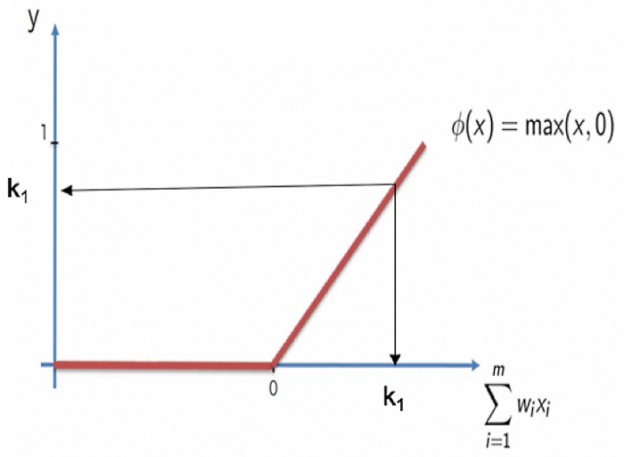
ReLU activation is summarized in the following diagram:
In other words, if x is equal to 0, then y must also be equal to 0. In other words, a signal that is less than zero or zero at the input will be translated into a zero output:
for
for
The moment x becomes greater than zero, it is x.
Neuronal networks commonly use the ReLU function for activation. Python can be used to implement it as follows:
The next step is to examine Leaky ReLU, which is based on ReLU.
Leaky ReLU
Negative values for x result in zero values for y in ReLU. It causes training cycles to be longer, especially at the beginning of training, since some information is lost in the process. This issue can be resolved by activating Leaky ReLU. Leaky ReLu entails the following:
; for
for
The diagram below illustrates this:
The parameter ß has a value less than one here.
Python can implement it as follows:
The value for ß can be specified in three ways:
The default value is ß, which we can specify.
In parametric ReLU, we let the neural network decide the value for ß (ß is a parameter in our neural network).
It is possible to make ß a random value (this is called randomized ReLU).
Tanh (hyperbolic tangent)
In addition to giving positive signals, the tanh function can also give negative signals. Here is a diagram that illustrates this:
Here is how the y function looks:
The following Python code can be used to implement it:
Taking a closer look at the softmax function now.
Softmax
Sometimes the activation function output requires more than two levels. As a result of Softmax, we can get a higher level of output than we would normally get from a two-level activation function. Multiclass classification problems are best suited to it. The number of classes is n. As input values, we have n. Class mapping is as follows:
x = {x(1),x(2),….x(n)}
Probability theory underpins Softmax’s operation. As a result, the softmax calculates the following output probability:
Binary classifiers use sigmoid activation functions, while multiclass classifiers use softmax activation functions.
Frameworks and tools
We will examine the frameworks and tools available for implementing neural networks in this section.
The implementation of neural networks has evolved over time using a variety of frameworks. There are strengths and weaknesses to different frameworks. Keras with a TensorFlow backend will be discussed in this section.
Keras
A popular neural network library written in Python, Keras is easy to use and popular. It provides the fastest way to implement deep learning and was designed with ease of use in mind. Models are considered at the model level with Keras because it only provides high-level blocks.
The Keras backend engines
In order to manipulate tensors at the tensor level, Keras needs a lower-level deep learning library. Backend engines are lower-level deep-learning libraries. The following engines can be used as Keras backends:
Among the most popular frameworks of this type, TensorFlow (www.tensorflow.org) is open-sourced and developed by Google.
At the MILA lab at Université de Montréal, this software was developed called Theona (deeplearning.net/software/theano).
Microsoft Cognitive Toolkit (CNTK): This is a Microsoft-developed tool.
The following diagram illustrates the modular structure of this deep learning technology stack:
By using a modular deep learning architecture, it is possible to change the backend of Keras without rewriting any code. Theona can be replaced with TensorFlow if we find it more suitable for a particular task than Theona.
Layers of the deep learning stack at the lowest level
Using the low-level layers of the stack, the three backend engines we just mentioned can all run on either CPUs or GPUs. On CPUs, Eigen is used to perform tensor operations. CUDA Deep Neural Network (cuDNN) is NVIDIA’s deep neural network library used by TensorFlow on GPUs.
Hyperparameter definition
Hyperparameters are parameters whose values are chosen before the learning process begins. The first thing we do is pick values that make sense to you, and then we optimize them later on. The following hyperparameters are important for neural networks:
Function of activation
Rate of learning
Layers hidden in the system
Each hidden layer has a certain number of neurons
Let’s take a look at how Keras can be used to define a model.
Modeling Keras
In order to define a complete Keras model, three steps are required:
Layers must be defined.
Keras can be used to build models in two ways:
A linear stack of layers can be architected using the Sequential API. The usual choice for building models is to use it for relatively simple models:
This has been done by creating three layers — the first two layer activation functions are ReLU and the third layer is softmax.
Acyclic graphs of layers can be architected using the Functional API. By using the Functional API, you can create more complex models.
There is no difference between the Sequential and Functional APIs when it comes to defining the same neural network. Model definition does not matter from a performance perspective.
The learning process should be defined.
Three things are defined in this step:
Optimizer
Loss function
Model quality will be quantified by the following metrics:
For the optimizer, loss function, and metrics, we use the model.compile function.
Model training.
The model needs to be trained once the architecture has been defined:
Hyperparameters such as batch_size and epochs can be configured.
Modeling sequentially vs. functionally
ANNs are created as simple stacks of layers in the sequential model. Despite its simplicity, the sequential model has a major limitation in terms of implementation and understanding. The input and output tensors of each layer are identical. A sequential model cannot be used if our model has multiple inputs or outputs, regardless of whether they are at the input or output or hidden layers. A functional model will be required in this case.
The TensorFlow API explained
There are many libraries available for working with neural networks, but TensorFlow is one of the most popular. In the previous section, we saw how to use it as Keras’ backend engine. Any numerical computation can be performed using this open source, high-performance library. The TensorFlow distributed execution engine can interpret high-level languages such as Python or C++ into TensorFlow code. Developers find it useful and popular for this reason.
A TensorFlow computation is represented by a Directed Graph (DG). Edges, inputs, and outputs of mathematical operations connect the nodes. Additionally, they represent data arrays.
Basic Concepts of TensorFlow
Let’s review TensorFlow concepts like scalars, vectors, and matrices. Simplified numbers, such as three and five, are known as scalars in mathematics. Additionally, a vector is something that has magnitude and direction in physics. A vector is a one-dimensional array in TensorFlow. Two-dimensional arrays can be considered matrices, extending this concept. Three-dimensional arrays are called 3D tensors. A data structure’s rank describes its dimensionality. The scalar data structure is ranked 0, the vector data structure is ranked 1, and the matrix data structure is ranked 2. Tensors are multidimensional structures, as shown in the following diagram:
Rank defines the dimensionality of a tensor, as shown in the diagram above.
The shape parameter is the next parameter to consider. An array’s shape is specified by a tuple of integers. Here is a diagram explaining the concept of shape:
In order to specify the details of tensors, we can use shape and rank.
The rest of the article is under a paid subscription. Writing this in-depth article takes time and a lot of effort. If you can help me keep up the momentum then please consider subscribing. It just costs you $5 and you will get the most in-depth article anywhere on the internet every day, sent directly to your inbox. Please consider subscribing it really helps.


