


Mastering Data Analysis With Pandas
A Complete Guide On How To Use Pandas For Data Aanalysis

Data science and Pandas
Recently, data science has become increasingly popular as a way to extract insights from data. Increasingly, businesses recognize the potential value of data and are investing in data scientists and technologies.
Making better business decisions is made possible by data science.
Data science has become popular due to easier access to, processing of, and transformation of data. The data comes from a variety of sources, including sensors, cash registers, credit card transactions, banks, etc. Raw data examples like these are all available online.
It is often necessary to handle some issues with raw data in order to make it usable. Raw data typically has the following issues:
Missing values.
Being stored with the wrong data type.
Not having a standard on the same type of values.
Noisy data.
This problem will be solved through data cleansing, but the process isn't exhaustive. Sometimes it is necessary to process data so that redundant information can be removed or more useful information can be extracted.
Consider the example of analyzing customer transaction data from a retailer. Our database contains information about the customer, the product purchased, the date of purchase, and so forth. Additionally, we are interested in how frequently customers visit the store. Calculate the time difference between two consecutive purchases of each customer to obtain this information. There is a lot of value in the data, but it needs a lot of cleaning and processing to be utilized.
Python's Pandas library provides data analysis and manipulation capabilities.
These operations are handled by Pandas, a Python library. Data cleaning, processing, and analysis are made easier and more efficient by their numerous functions and methods. Pandas provide straightforward solutions to complex problems with a simple and clear syntax.
Data cleaning and processing consume a large amount of time in the data science workflow. In data science, Pandas is a useful and practical tool. You need an introductory level of Python knowledge in order to benefit from this article.
What Will You Achieve by Completing This Article?
Learn what Python Pandas offers.
Pandas library
All data analysis and manipulation needs are met by Pandas, a highly functional and efficient library. In this course, we'll learn how to use Pandas to accomplish the following tasks:
Handle missing values.
Filter data based on the desired conditions.
Remove noise from data.
Manipulate strings or textual data.
Manipulate dates and times.
Analyze data to extract insights and more useful information.
Visualize data to understand it thoroughly.
Combine data from different resources.
A variety of advanced tasks require these operations, such as segmenting customers, predicting churn, and analyzing time series. Our raw data needs to be cleaned and processed in order to accomplish these tasks.
Let's say we're trying to solve a machine-learning problem. A machine learning algorithm expects input data to be formatted in a certain way. Data cannot be cleaned or processed by these algorithms. The data must be formatted for the algorithm. We're likely to get unsatisfactory results when feeding raw data to a machine-learning algorithm. Machine learning also requires data cleaning and processing.
Practicing a software tool or library is the best way to learn it. To explore Pandas' functions and methods, we'll look at several examples and challenges.
Pandas Data Structures
Pandas Series
Learn Series - the one-dimensional data structure of Pandas
What is Series in Pandas?
There are axis labels on a series, which is a one-dimensional array. Arrays can be created in several ways. Pandas must be imported before we can begin exploring the examples.
import pandas as pdPython libraries are typically aliased when imported. PD is used for Pandas, but anything can be assigned. If you assign a different alias, make sure to replace pd in the examples with the one you used.
import pandas as pd

myseries = pd.Series([10, 20, 30])

print(myseries)
The index parameter can be used to change the index assigned to Series by default.
import pandas as pd

myseries = pd.Series(
     [10,20,30],
     index = ["a","b","c"]
)

print(myseries)
We can access the items in a Series with their index.
import pandas as pd

myseries = pd.Series(
   ["Jane","John","Emily","Matt"]
)

# Print the first item
print(myseries[0])
A Python dictionary or NumPy array can also be used to create the Series index. It is just a matter of passing them to the Series constructor as we have done so far. Series can be used with several Pandas methods and functions.
Here are a few examples to illustrate these methods. Using the is_unique method, a series is checked to see if there are duplicate items.
import pandas as pd

myseries = pd.Series([1,2,3])
print(myseries.is_unique)
In this lesson, we’ve learned what a Series is, how to create one, and how to apply a function to a Series.
Pandas DataFrame
DataFrame, Pandas' two-dimensional data structure, is what you need to know.
What is DataFrame in Pandas?
Pandas uses DataFrames as two-dimensional data structures. Columns and rows are labeled.
Here is a simple example to help you understand the basic features of a DataFrame. A Python dictionary can be passed to the constructor of a DataFrame in order to create it.
import pandas as pd

df = pd.DataFrame({
    "Name": ["Jane", "John", "Matt", "Ashley"],
    "Age": [24, 21, 26, 32]
})

print(df)
Dictionary keys are used to name columns, and data is stored in a DataFrame using the values in the dictionary. Having two columns and four rows, we now have a DataFrame. Using a DataFrame's shape method, we can find out how many rows and columns there are.
import pandas as pd

df = pd.DataFrame({
    "Name": ["Jane", "John", "Matt", "Ashley"],
    "Age": [24, 21, 26, 32]
})

print(df.shape)
Tabular data can be manipulated and analyzed using Pandas' numerous functions and methods.
Exploring a Data Frame
Reading Data from a File
Learn how to create a Pandas DataFrame from data in a file.
Reading data from a csv file#
Our most common method of reading data is from a file. A CSV file format is most commonly used, as well as an Excel file format, a Parquet file, and a JSON file. CSV files will be used in this course. A DataFrame is created from a CSV file using the pandas read_csv function. In addition to read_json, read_parquet, and read_excel, Pandas provides several other functions for reading data.
Here is an example of how to use the read_csv function. Only the file path, relative to the current working directory, is required as a parameter. We simply need to provide the function with the file name if the file is in the current working directory.
For an overview of the dataset, the head method returns the first five rows of the DataFrame.
import pandas as pd

sales = pd.read_csv("sales.csv")

print(sales.head())
Using usecols parameter
The read_csv function also has several parameters. The csv file can be read only by some columns, for instance.
import pandas as pd

sales = pd.read_csv("sales.csv", usecols=["product_code","product_group","stock_qty"])

print(sales.head())
Rows and columns make up a DataFrame. We can limit the number of rows read by the read_csv function by using the nrows parameter, just as we can limit the columns. It's especially useful when you're dealing with large files. Assume that there are 10 million rows in a file. If we want to read only 1000 rows in the file for a quick analysis or exploration, we can set the nrows parameter to 1000.
Create a DataFrame
Use different data structures to create a DataFrame. Pandas allows you to create your own DataFrame, even though we usually read data from an external file.
Python dictionary
Python dictionaries are one of the most commonly used methods. Constructing a DataFrame just requires passing a dictionary.
import pandas as pd

df = pd.DataFrame({
  "Names": ["Jane", "John", "Matt", "Ashley"],
  "Ages": [26, 24, 28, 25],
  "Score": [91.2, 94.1, 89.5, 92.3]
})

print(df)
Two-dimensional array
Rows and columns make up a DataFrame, a two-dimensional data structure. DataFrames are created by converting two-dimensional arrays. It is possible to construct a DataFrame using NumPy arrays, for example.
A NumPy array is used in the code below to create a DataFrame. A column name is assigned an integer index by default, but this can be changed by using the columns parameter.
import numpy as np
import pandas as pd

arr = np.random.randint(1, 10, size=(3,5))

df = pd.DataFrame(arr, columns=["A","B","C","D","E"])

print(df)
We’ve seen how to create a DataFrame using Python dictionaries and NumPy arrays.
Exploring a Data Frame
Size of a DataFrame
Learn how to determine the size of a Pandas DataFrame.
The size, shape, and len methods
It is always a good idea to check the size of the data before analyzing it. Rows and columns can be used to express the size of a DataFrame.

A DataFrame with 5 rows and 4 columns
A tuple containing the number of rows and columns is returned by the shape method. A number is returned by the size method that represents the number of rows multiplied by the number of columns. As a result, it returns the total number of cells in a DataFrame. Using the built-in Python function, len, we can find out how many rows there are in a DataFrame. These methods can be used to determine the sales size.
import pandas as pd

sales = pd.read_csv("sales.csv")

print(sales.shape)

print(sales.size)

print(len(sales))
The len function can be used if all we are interested in is the number of rows in a DataFrame. Tuples returned by the shape method contain both rows and columns. The size method is rarely used.
Data Types of Columns
Learn how to find and change the data types of columns in Pandas.
Data types
Numbers aren't always the only way to represent data. We must also deal with strings (textual data), dates, times, and boolean (True or False) data types in addition to integers and floats.
It’s important to use proper data types for two main reasons:
Different types of data structures require different amounts of memory. Memory can be saved by using proper data types.
It is also possible to use some methods and functions with certain types of data. It is necessary to store data containing date and time in the datetime data type in order to use it.
The first thing we need to do is check the types of data in the sales. Let's look at changing column data types next.
import pandas as pd

sales = pd.read_csv("sales.csv")

print(sales.dtypes)
The dtypes method returns the data type of all columns.
Changing the data type
The first thing we need to do is check the column names in a DataFrame. A DataFrame can be displayed by using the head method for the first five rows.
The columns method is a more practical approach. Using the list function, we can convert the columns into a list.
import pandas as pd

sales = pd.read_csv("sales.csv")

print("As index:")
print(sales.columns)

print("As list:")
print(list(sales.columns))
Integers are used as the data type for the stock quantity column. Let's say we have products whose stock amounts are decimal points. The amount of rice we have, for example, might be 125.2 kg.
We can use the astpye function to change the data types of columns.
import pandas as pd

sales = pd.read_csv("sales.csv")

sales["stock_qty"] = sales["stock_qty"].astype("float")

print(sales.dtypes)
By using the astype function, we can change the data type of multiple columns at once. Dictionary keys indicate new data types for column names and values.
"Stock quantity" and "last week's sales" should both be changed to a different type of data.
import pandas as pd

sales = pd.read_csv("sales.csv")

sales = sales.astype({
  "stock_qty": "float",
  "last_week_sales": "float"
})

print(sales.dtypes)
Both columns now have the float data type.
Different Values in a Column
A Pandas DataFrame column can be sorted by distinct values.
Using the unique and nunique functions
A DataFrame can contain categorical or continuous columns. Continuous columns can have infinite numbers of values, whereas categorical columns can have many distinct but finite values. As such, the columns can be viewed as either discrete or categorical random variables.
An essential part of exploratory data analysis is checking the number of distinct values in a categorical column. The unique function actually shows the unique values in a column, while the nunique function returns the number of distinct values in a column. They can be applied to the sales column for product groups.
import pandas as pd

sales = pd.read_csv("sales.csv")

print(sales["product_group"].nunique())

print(sales["product_group"].unique())
The value_counts function
The product line is divided into six distinct groups. The number of rows in each product group might also need to be checked. The value_counts function returns all the distinct values in a column along with the number of their occurrences.
import pandas as pd

sales = pd.read_csv("sales.csv")

print(sales["product_group"].value_counts())
Pandas' value_counts function is a popular way to explore categorical columns quickly.
Measures of Central Tendency
The mean, median, and mode
A measure of central tendency is the mean, median, and mode, which provides insight into a variable's distribution.
An average value is referred to as the mean. You can calculate it by adding all the numbers in a dataset and dividing the sum by the number of values in the dataset.
If the values are sorted ascendingly or descendingly, the median value represents the middle value. Medians are averages of the two middle values in a dataset with an even number of values.
A Series with six values, for example, can be seen below. Make sure the median is the average of the two middle values by running the code.
import pandas as pd

myseries = pd.Series([1, 2, 5, 7, 11, 36])

print(myseries.median())
An example of a mode is the most frequent value in a dataset. The mode of a dataset can be found by running a simple example.
import pandas as pd

myseries = pd.Series([1, 4, 6, 6, 6, 11, 11, 24])

print(f"The mode of my series is {myseries.mode()[0]}")
In categorical data, only the mode is applicable, while mean and median are only applicable to numerical data. When a restaurant's most popular burger is represented by the mode of the dataset that contains all of the burgers sold there, not the entire town.
The minimum and maximum values might also be important when exploring the data.
Let's calculate the central tendency and minimum and maximum values for the price column in the sales.
import pandas as pd

sales = pd.read_csv("sales.csv")

print("mean: ")
print(sales["price"].mean())

print("median: ")
print(sales["price"].median())

print("mode: ")
print(sales["price"].mode()[0])

print("minimum: ")
print(sales["price"].min())

print("maximum: ")
print(sales["price"].max())
Approximately 67 is the average price, and 23 is the median price. As a result, some of our products have a higher price.
Descriptive statistics rely heavily on measures of central tendency. It is also important to take into account the variance or standard deviation of a variable in order to gain a deeper understanding of its distribution.
Variance measures how values differ. The following formula can be used to calculate it:
Find the difference between each value in the dataset and the mean.
Take the square of the differences.
Find the average of the squared differences.
In mathematics, standard deviation measures the spread of values. More specifically, it is variance squared.
Variance and standard deviation can be calculated using Pandas' var and std methods.
import pandas as pd

sales = pd.read_csv("sales.csv")

print("variance: ")
print(sales["price"].var())

print("standard deviation: ")
print(sales["price"].std())
It is possible to figure out how the values are spread out around the central tendency by looking at the variance and standard deviation. Standard deviation generally indicates how spread out the values are.
Filtering a Data Frame
Why Do We Need Filtering?
Explore the cases in which a Pandas DataFrame needs to be filtered.
DataFrames are commonly filtered. In essence, it involves excluding some values to meet a condition.
When to filter a DataFrame?
We may need to filter for several reasons:
Data can be filtered when redundant or unnecessary information needs to be removed. Imagine we're predicting customer churn with machine learning. This case requires filtering out the bank account number of the customer.
Imagine working at a bank as a data analyst. A promotion will be announced for customers who meet certain criteria regarding account balances, monthly spending, and products (a credit card or checking account). In order to find customers eligible for the promotion, the data analyst needs to filter the data.
Data manipulation and cleaning require filtering as well. If some columns of a DataFrame have missing values, we might want to filter them out.
As well as in data analysis, filtering is frequently used. Imagine that we're grouping customers based on how much they spend. As an example, we filter customers based on how much they spend and then group them based on how much they spend.
There are two ways to filter: by observations (rows) or by features (columns). The good news is that Pandas has a lot of flexibility and efficiency for such operations.
A DataFrame can be filtered in both rows and columns using various methods in this chapter.
Filtering with "loc" and "iloc" Methods
Learn about the loc and iloc methods of Pandas.
The loc and iloc methods
Data manipulation, filtering, and selection are all accomplished with the loc and iloc methods in Pandas. By using them, we can access any combination of rows and columns that are desired.
Rows and columns are accessed differently by them:
locuses row and column labels.ilocuses row and column indexes.
The following illustration illustrates a DataFrame. By using index values (0, 1, and 2), we can access rows and columns using the iloc method. The loc method requires labels A, Day 1, etc.) if we want to use it.
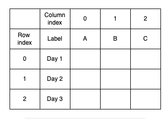
A DataFrame's index and labels
For the first step, we will use the loc method to select the first five rows and two columns from the sales report.
import pandas as pd

sales = pd.read_csv("sales.csv")

print(sales.loc[:4, ["product_code","product_group"]])
In this case, the :4 indicates the rows starting at 0 and 4 in the row sequence, which is the equivalent of 0:4. The loc method receives the column names as a list. Iloc can also be used to perform the same operation.
import pandas as pd

sales = pd.read_csv("sales.csv")

print(sales.iloc[[5,6,7,8], [0,1]])

print(sales.iloc[5:9, :2])
There is a similar effect in lines 5 and 7. In a list, however, passing indices as [5,6,7,8] is a more convenient approach than passing the indices as [5,6,7,8].
//
I would like to point out that both the loc and iloc were selected in the same manner. By default, Pandas labels rows with integers. If you do not specify otherwise, the indexes and labels of each row will be the same, unless we specify otherwise. To see the difference more clearly, I will create a custom index for the data frame.
Frequently, loc and iloc methods are used to select or extract portions of a data frame. Unlike loc, iloc uses indices instead of labels.
import numpy as np
import pandas as pd

df = pd.DataFrame(
  np.random.randint(10, size=(4,4)),
  index = ["a","b","c","d"],
  columns = ["col_a","col_b","col_c","col_d"]
  )

print(df)

print("\nSelect two rows and two columns using loc:")
print(df.loc[["b","d"], ["col_a","col_c"]])
The loc and iloc methods can be used to select or extract a data frame. Loc uses labels, while iloc uses indices, which is the main difference between them.
Filtering by Selecting a Subset of Columns
It is possible to filter Pandas DataFrames based on subsets of columns.
Selecting a subset of columns
In real-life datasets, there are likely to be several columns. Some of them may be redundant, so we may not need to include them in our analysis. In such cases, you can select a subset of columns. Filtering the column names is as simple as writing them into a list.

Below is a code snippet that selects the columns product code and price in the sales column.
import pandas as pd

sales = pd.read_csv("sales.csv")

selected_columns = ["product_code","price"]

print(sales[selected_columns].head())
The names of the columns do not need to be listed. The same operation can also be performed using this line:
print(sales[["product_code","price"]].head())Column names should be written in a list. Due to Pandas' interpretation of the string as one column, we'll end up with an error. By executing the following code snippet, you can see the generated error.
import pandas as pd

sales = pd.read_csv("sales.csv")

print(sales["product_code","price"].head())
If only one column needs to be selected, a list must be placed. A DataFrame with just one column will be returned instead if Pandas returns a Series.
Filtering by Condition
Use a condition or a set of conditions to filter values in a DataFrame.
How to filter a DataFrame by condition
Let's take a moment to reflect on what we've been using for sales. Six product groups are divided among the products. Let's say we want to filter products that belong to only one product category.
The following line of code selects the products of the PG2 product group. The sales table has rows for each product.
sales_filtered = sales[sales.product_group == "PG2"]
The same function is performed by this line of code.
sales_filtered = sales[sales["product_group"] == "PG2"]
Any of the options above can be used if the column name contains a space. As a result, the first option is unlikely to be effective.
DataFrames can also be filtered using numerical values. A code that selects products with prices greater than 100 is shown below.
sales_filtered = sales[sales["price"] > 100]
Conditions can be created using the following operators:
==: equal!=: not equal>: greater than>=: greater than or equal to<: less than<=: less than or equal to
Multiple conditions
It is possible to filter a DataFrame using multiple conditions. Pandas' library supports logical operators for combining filters.
A product with a price higher than 100 and a stock quantity less than 400, for example, could be selected. These conditions must be combined with the & operator.
import pandas as pd

# read the sales csv file
sales = pd.read_csv("sales.csv")

# filter the sales data frame
sales_filtered = sales[(sales["price"] > 100) & (sales["stock_qty"] < 400)]

print(sales_filtered[["price","stock_qty"]].head())
When multiple conditions are combined, the filters need to be enclosed in parentheses. An error will occur if this is not present.