Mastering Financial Data Analysis: From Python Libraries to LSTM Models

A Comprehensive Guide to Data Handling, Visualization, and Predictive Modeling in Finance

This article explores the critical tools and techniques for effective financial data analysis using Python. From importing essential libraries to developing and visualizing LSTM models, we cover the fundamentals of handling, analyzing, and predicting financial data trends. Whether you’re retrieving historical stock prices or calculating technical indicators, this guide provides the insights needed to enhance your data analysis skills in the financial domain.

Import libraries for data analysis

import numpy as np
import pandas as pd
import matplotlib.pyplot as plt
import seaborn as sns
import datetime 
from datetime import date
import math
import pandas_datareader as web

The snippet of code includes the importation of diverse Python libraries tailored for handling data, crafting visual representations, and conducting analyses.

- Numpy, proficient at executing numerical operations on arrays and matrices.

- Pandas, which equips users with data structures and analytical resources suitable for managing structured data.

- Matplotlib.pyplot, a plotting tool capable of generating an array of graphs like line plots, bar charts, and histograms.

- Seaborn, a data visualization platform built on top of matplotlib that furnishes an intuitive interface for creating visually appealing and informative statistical graphics.

- Datetime, a Python module that provides classes to manage dates and times effectively.

- Pandas_datareader, a library designed to fetch data from a variety of online sources into a pandas DataFrame.

Through the incorporation of these libraries, the code establishes a Python setting conducive to loading, examining, and visualizing data with efficiency. These libraries contain a broad spectrum of functionalities and utilities for processing and investigating data, simplifying the extraction of meaningful insights from the dataset.

Preprocessing and defining LSTM model architecture

from sklearn.preprocessing import MinMaxScaler
from keras.models import Sequential
from keras.layers import Dense
from keras.layers import LSTM
from keras.layers import Dropout

In this script, we are importing crucial modules and functions from the scikit-learn library (specifically MinMaxScaler) and the Keras library (including Sequential, Dense, LSTM, Dropout).

- MinMaxScaler plays a pivotal role in scaling features within a specified range, commonly within 0 and 1.

- The Sequential component is instrumental in establishing a linear sequence of layers in a neural network.

- To set up a fully connected layer within a neural network, we utilize Dense.

- LSTM, or Long Short-Term Memory, is utilized for developing LSTM layers within a neural network, enabling the model to grasp extended patterns in data sequences.

- In order to prevent overfitting by randomly nullifying a portion of input units during each training update, we employ Dropout.

These tools are fundamental when constructing and training neural network models, especially beneficial for deep learning assignments like predicting time series, language processing, and image recognition. Leveraging these libraries allows you to effectively craft robust deep learning models.

Retrieve and display historical stock prices

data = web.get_data_yahoo('^NSEBANK', start = datetime.datetime(2000, 1, 2), 
                             end = date.today())
data = data[['Adj Close']]
data.columns = ['Price']
data.head()

The following code segment is designed to extract historical stock information for the Nifty Bank index from the Yahoo Finance API, focusing on the ‘Adj Close’ price starting from January 2, 2000, up to the present day.

This script leverages the web.get_data_yahoo() function available in the pandas_datareader library to pull stock data from Yahoo Finance, with ^NSEBANK serving as the symbol for the Nifty Bank index. By defining start and end dates to pinpoint the data range, encompassing January 2, 2000, to today’s date through the utilization of date.today(), it homes in on the ‘Adj Close’ prices exclusively. Renaming the column as ‘Price’ enhances data interpretation, followed by a data.head() call to exhibit the initial data rows retrieved.

This code snippet proves instrumental in accessing historical stock market insights pivotal for analytical, visualization, and modeling purposes within financial arenas. It effectively captures the adjusted closing cost trend of the Nifty Bank index, facilitating a comprehensive evaluation of this specific financial indicator’s performance trajectory across time.

Prints number of days in dataset

print('There are {} number of days in the dataset.'.format(data.shape[0]))

The following code snippet serves the purpose of revealing the count of rows within a dataset. Let’s break down its functionality:

- Utilizing data.shape[0] enables the retrieval of the row count within the dataset labeled as data.

- By implementing the format() method, the obtained number is seamlessly inserted into the designated placeholder {} found within the string “There are {} number of days in the dataset.”

- Ultimately, the print() function executes the task of displaying the complete string, inclusive of the count of days, to the console.

This code proves to be advantageous when aiming to furnish insights regarding the dataset’s scale or proportions in a manner easily comprehensible to users. It bolsters the user experience by presenting pertinent dataset specifics in a user-friendly format.

Plotting Bank Nifty price against date

plt.figure(figsize=(28, 12))
plt.plot(data.index, data['Price'], label='Bank Nifty Price')
plt.xlabel('Date')
plt.ylabel('Rs')
plt.title('Bank Nifty Price')
plt.legend()
plt.show()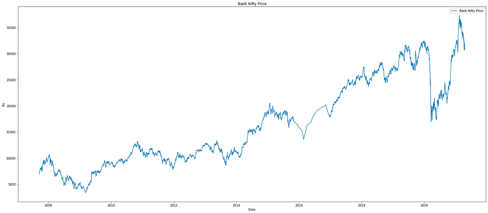

This snippet of code serves the purpose of generating and showcasing a line graph illustrating Bank Nifty price data over different dates. Let’s delve into the breakdown of each component within the code: