


Mastering Pairs Trading: A Guide to Algorithmic Strategies in the Stock Market
Mastering Pairs Trading: A Guide to Algorithmic Strategies in the Stock Market
Exploring the Dynamics of Stock X and Stock Y Through Algorithmic Trading Techniques

In the intricate world of stock trading, understanding the nuances of market behavior is crucial for success. This article delves into the fascinating realm of algorithmic trading, focusing on the concept of pairs trading — a strategy that involves two interconnected stocks, named here as Stock X and Stock Y. By analyzing their historical price movements and employing techniques like mean reversion and cointegration, we unravel how algorithmic trading can be leveraged to predict and capitalize on stock market trends. The article also introduces practical tools and programming libraries, such as Python’s Pandas, NumPy, Matplotlib, and yfinance, demonstrating how they can be effectively used to retrieve, clean, normalize, and analyze financial data. Whether you’re a seasoned trader or a novice in the world of algorithmic trading, this guide offers valuable insights into mastering pairs trading and making informed decisions in the stock market.
Download the source code from the link at the end of this article.
Imagine there are two stocks, let’s call them Stock X and Stock Y, from companies that are connected in some way. They might be in the same industry, rely on each other for materials, or sell to the same type of customers. Up until a certain point in time, which we’ll call ‘Time i’, the prices of Stock X and Stock Y usually move in the same direction. But, as often happens in the stock market, even related stocks can start to behave differently due to various reasons like a new product release, negative publicity, or low profits. At Time i, the difference in their prices is the largest.
There’s a concept in stock trading called ‘Mean Reversion’ which suggests that over time, these stocks will return to their average behavior. So, after Time i, we expect Stock Y to decrease in price and Stock X to increase. Knowing this, a trader could bet on this by ‘going short’ on Stock Y (betting its price will fall) and ‘going long’ on Stock X (betting its price will rise). When the stocks return to their average behavior, which is after Time i, the trader can close their positions and potentially make a profit.
The advantage of “pairs trading,” where you trade two related stocks together, is that it’s less risky in terms of potential losses. Let’s say after a certain time, which we’ll call ‘Time i’, both Stock Y and Stock X start to increase in price. In this case, the money you make from the stock you bet would rise (your ‘long’ position) could balance out any loss from the stock you bet would fall (your ‘short’ position). Similarly, if after Time i, both stocks start to decrease in price, the money you make from your ‘short’ position could cover the loss from your ‘long’ position.
Another good thing about pairs trading is that it’s not very affected by general market trends. This strategy focuses on the price differences between two connected stocks, not the overall market. So, even if the market as a whole is going up or down, these two stocks will likely move together. As explained earlier, this can still lead to a profit, regardless of whether the overall market is trending upwards or downwards.
Retrieve, Clean And Normalize
import pandas as pd
import numpy as np
import matplotlib.pyplot as plt
import yfinance as yf
Matplotlib.pyplot, pandas, numpy, and yfinance make up this code. Python provides functions and data structures for manipulating, analyzing, and visualizing data. A pandas and numpy module can be referred to easily by using the pd and np aliases, respectively. It’s used to access the matplotlib.pyplot module that provides tools for creating data visualizations. This alias is used by the yfinance module, which allows users to access financial data on Yahoo! A financial API. There is nothing else that the code does after importing these modules. In this case, it simply makes these functions and data structures available to the Python session for use. It is possible to manipulate and analyze data using these modules by calling specific functions or using specific data structures, such as creating data frames using pandas or plotting data using matplotlib.pyplot. Yahoo’s financial data can be retrieved using the yfinance module! Analysis of finance using the other modules.
Using our understanding, we can try to predict two stocks that might behave similarly. For example, Tesla and JPMorgan, both of which are publicly traded, could potentially move together. This might happen because JPMorgan could have investments in major stocks like Tesla, which is part of the S&P 500 index. So, the way Tesla’s stock performs could influence JPMorgan’s success and, in turn, its own stock price. Let’s explore if they make a good pairing for trading!
# Note: we only want the adjusted close data, ytd
STOCK_A = 'TSLA'
STOCK_B = 'JPM'
raw_data = yf.download(tickers=[STOCK_A, STOCK_B], period='ytd', interval='1d')
raw_data = raw_data.drop(columns=['Close', 'High', 'Low', 'Open', 'Volume'])

# Getting rid of 'TSLA' and 'JPM' as sub-columns under 'Adj Close'... making them separate columns
data = pd.DataFrame()
data[STOCK_A] = raw_data['Adj Close'][STOCK_A]
data[STOCK_B] = raw_data['Adj Close'][STOCK_B]

data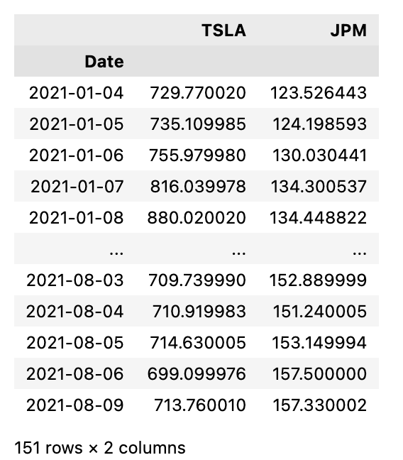
The first thing this python code does is define two variables: STOCK_A = TSLA and STOCK_B = JPM. The following symbols represent the stock ticker symbols for Tesla and JPMorgan Chase, respectively. Next, stock data for these two tickers is downloaded using the yfinance library. Using the parameters specified suggests downloading the data for the year-to-date ytd period with a daily interval. Known as raw_data, this data is stored in a variable.
Next, we drop useless columns from the raw data, specifically Close, High, Low, Open, and Volume. The only column left is the Adj Close column, which displays the adjusted closing prices of each stock on any given day. In the next line, we create a new dataframe in pandas. All that will be contained in this dataframe is the updated close data for the two tickers. Data dataframes are used in the following two lines of code to store adjusted close data.
As soon as the raw_data dataframe is loaded, TSLA is added as a column to the data dataframe as the Adj Close data for the STOCK_A ticker. Similarly, the second line does the same thing for the ticker STOCK_B. The code downloads adjusted close data for Tesla and JPMorgan Chase, for the year-to-date period, into a dataframe for analysis.
plt.figure(figsize=(12,5))
axis1 = data[STOCK_A].plot(color='blue', grid=True, label=STOCK_A)
axis2 = data[STOCK_B].plot(color='green', grid=True, label=STOCK_B)
h1, l1 = axis1.get_legend_handles_labels()
h2, l2 = axis2.get_legend_handles_labels()
plt.legend(h1, l1, loc=2)
plt.title(label='Non-Normalized TSLA and JPM Stock Prices ($)')

plt.show()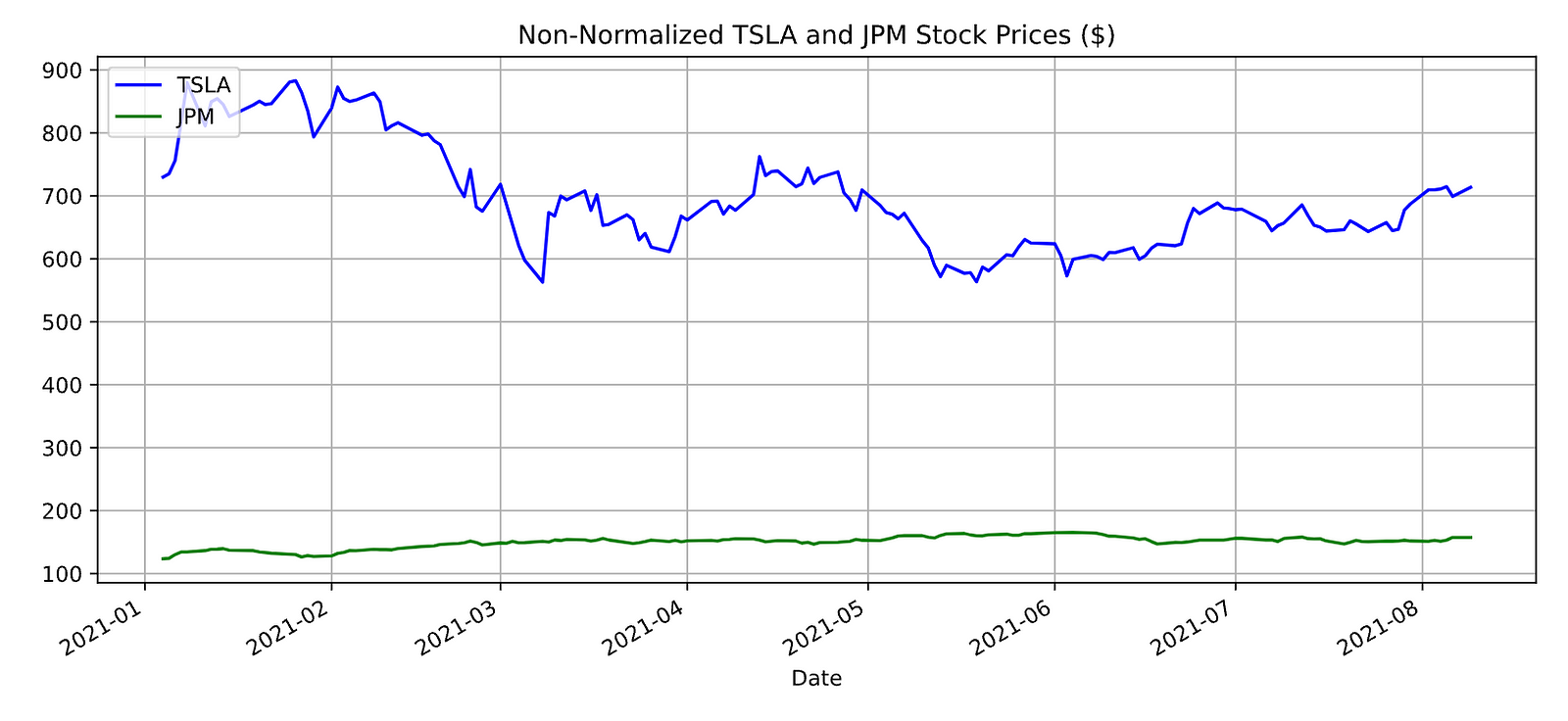
A figure with a specific size of 12 x 5 inches is created with this code using the matplotlib library. STOCK_A and STOCK_B are set up in the figure as separate axes. Stock data is plotted on their respective axes in a specified color and grid pattern. As a next step, the code stores the legend handles h1 and h2 for each stock and labels l1 and l2 for each stock. Later, the plot’s legend will be created based on these. Plot.legend is then used to add a legend to each plot, using the previously stored handles and labels. Locate the plot’s legend in the upper left corner with the loc=2 parameter. Using plt.show, the code provides a title for the plot. It creates a plot with two stock prices and adds a legend and title so that the data is better visualized.
# Normalize the the dataframe using cumulative percentage change
norm_data = pd.DataFrame()

norm_data[STOCK_A] = data[STOCK_A].pct_change().cumsum()
norm_data[STOCK_B] = data[STOCK_B].pct_change().cumsum()

# The first row will contain NaN, since there is no previous row to calculate percent change
norm_data = norm_data.tail(len(data) - 1)

norm_data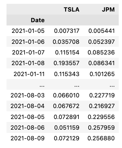
This code creates a new table that contains the normalized data that is calculated for two specific stocks: STOCK_A plus _norm, STOCK_B plus _norm. Norm_data is an empty dataframe created with two columns, STOCK_A and STOCK_B. Following are two lines that calculate the percentage change for each stock and apply the cumsum function. Accordingly, each value in the dataframe represents the total percentage change since the first value. A percent change is calculated from the next row of the dataframe, since the first row contains NaN values. As a final step, the last line renames the columns of the dataframe to indicate that they contain normalized data. Using this code, two different stocks can be compared by normalizing their data and representing their percentage change relative to their initial values.