Mastering Portfolio Optimization: Balancing Risk and Return

Techniques and Strategies for Maximizing Investment Returns

Portfolio optimization is a critical component of modern investment management, focusing on the strategic allocation of assets to achieve the best possible balance between risk and return. This process involves selecting a mix of investment assets that maximizes an investor’s expected returns for a given level of risk or, conversely, minimizes risk for a given level of expected return. The foundation of portfolio optimization lies in Markowitz’s Modern Portfolio Theory (MPT), which introduces the concept of diversification to reduce risk. By carefully analyzing the correlations between asset returns, investors can construct portfolios that mitigate unsystematic risk and improve overall performance.

Recent advancements in computational finance and data analytics have significantly enhanced the techniques and tools available for portfolio optimization. Sophisticated models now incorporate various constraints and objectives, such as minimizing drawdowns, achieving specific liquidity targets, or adhering to regulatory requirements. Techniques like mean-variance optimization, factor models, and machine learning algorithms provide robust frameworks for optimizing portfolios under complex market conditions. This article delves into these methods, illustrating their practical applications through simulations and real-world examples, and highlighting how investors can leverage these strategies to achieve superior investment outcomes.

Link to download source code at the end of this article.

Onepagecode is a reader-supported publication. To receive new posts and support my work, consider becoming a free or paid subscriber.

---

Imports necessary Python packages for analysis

# Imports from Python packages.
import matplotlib as mpl
import matplotlib.pyplot as plt
from matplotlib.ticker import FuncFormatter
from matplotlib.lines import Line2D
import multiprocessing as mp
import seaborn as sns
import pandas as pd
import numpy as np
import pygmo as pg
import os
import time
from numba import jit
from scipy.stats import norm
from datetime import timedelta
from functools import partial
from itertools import chain, combinations

The given code snippet imports various Python libraries and modules to enhance a Python script or program. It includes matplotlib, which is a plotting library used for creating visualizations such as charts, graphs, and histograms. The multiprocessing module supports concurrent execution using processes instead of threads, while seaborn, built on top of matplotlib, is utilized for creating more attractive and informative statistical graphics.

Pandas is a library for data manipulation and analysis, especially with labeled data structures like DataFrames. Numpy, the fundamental package for scientific computing, provides support for large, multi-dimensional arrays and matrices. Pygmo, a Python library, aids in general-purpose global optimization using evolutionary algorithms. The os module offers a portable way to use operating system-dependent functionalities, and the time module includes functions related to time.

Additionally, numba acts as a Just-In-Time (JIT) compiler for Python functions to enhance performance. The scipy.stats submodule from SciPy is used for statistical functions and probability distributions. For working with date and time, the datetime module is employed. Functools provides higher-order functions and operations on callable objects, whereas itertools offers efficient looping constructs.

This Substack is reader-supported. To receive new posts and support my work, consider becoming a free or paid subscriber.

By importing these libraries, the code gains access to a wide range of functionalities necessary for data processing, visualization, optimization, parallel processing, statistical analysis, and computational efficiency. Each library serves a specific purpose, collectively offering a versatile toolkit for various data science and scientific computing tasks.

Imports various functions for financial operations

# Imports from FinanceOps.
import diversify
from portfolio_utils import (normalize_weights, weighted_returns,
    fix_correlation_matrix, check_correlation_matrix)
from returns import max_drawdown, max_pullup
from stats import normal_prob_loss, normal_prob_less_than
from utils import linear_map

This code snippet imports various functions and modules from different files, including diversify, portfolio_utils, returns, stats, and utils, each providing specific functionalities related to financial operations and calculations. The diversify module primarily contains functions related to diversification. Portfolio_utils offers functions for managing portfolios, such as normalizing weights, calculating weighted returns, fixing correlation matrices, and checking correlation matrices. The returns module focuses on calculating financial indicators like maximum drawdown and maximum pullup. The stats module is used to compute statistics such as the normal probability of loss and normal probability less than specific values. Lastly, the utils module consists of general utility functions like linear mapping. These imports are crucial for modularizing finance-related operations, effectively organizing the codebase, reducing redundancy, and facilitating a structured approach to developing financial operations.

Imports SimFin data and functions

# Imports from SimFin.
import simfin as sf
from simfin.names import (TOTAL_RETURN, CLOSE, VOLUME, TICKER,
                          PSALES, DATE)
from simfin.utils import BDAYS_PER_YEAR

This code snippet imports essential functions and variables from the SimFin library, facilitating access to financial data, such as stock prices, fundamental data, and other financial metrics. The imported variables — including TOTAL_RETURN, CLOSE, VOLUME, TICKER, PSALES, and DATE — represent the names of columns in a financial dataset, enabling easy reference to specific columns. Additionally, the variable BDAYS_PER_YEAR likely stores the number of business days in a year, a common parameter in financial calculations.

Utilizing these imported functions, variables, and dataset names simplifies financial analyses, calculations, and data manipulations, contributing to more efficient and cleaner code. Furthermore, employing meaningful variable names enhances code readability and mitigates potential errors that could arise from manual entry of column names or other data-related details.

Generates random numbers with a seed

# Random number generator.
# The seed makes the experiments repeatable. In the year 1965
# the scientist Richard Feynman was awarded the Nobel prize in
# physics for discovering that this particular number was the cause
# of "The Big Bang" and all that matters in the entire universe.
rng = np.random.default_rng(seed=81680085)

The provided code snippet initializes a random number generator using the NumPy library with a specific seed value. Using a seed value makes the generation of random numbers reproducible, ensuring that if you run the same code with the same seed multiple times, you will get the same sequence of random numbers. This reproducibility is particularly useful for debugging or testing code that involves randomness, as it allows the recreation of the same random conditions.

In this instance, the seed value chosen is 81680085. A comment within the code humorously attributes the cause of The Big Bang and all universal matter to this specific number. While not scientifically accurate, this playful remark underscores the significance of the seed in random number generation.

Creates directory for storing plots

# Create directory for plots if it does not exist already.
path_plots = 'plots/portfolio_optimization/'
if not os.path.exists(path_plots):
    os.makedirs(path_plots)

This code snippet ensures that a directory for storing plots related to portfolio optimization exists. It checks if the specified directory path (‘plots/portfolio_optimization/’) is already present using the os.path.exists() function. If the directory does not exist, it creates it using os.makedirs(). This step is crucial because it is necessary to confirm that the directory where files will be saved is available. By creating the directory if it doesn’t exist, this code prepares the required structure for storing the plots generated during the portfolio optimization process and ensures that no errors occur due to missing directories when attempting to save the plots.

Sets SimFin data directory and loads API key

# SimFin data-directory.
sf.set_data_dir('~/simfin_data/')

# SimFin load API key or use free data.
sf.load_api_key(path='~/simfin_api_key.txt', default_key='free')

This code snippet is from a financial data library called SimFin, which provides access to company financial data. The first line, sf.set_data_dir(‘~/simfin_data/’), sets the directory where SimFin data will be stored or accessed, in this instance directing it to ‘~/simfin_data/’. The second line, sf.load_api_key(path=’~/simfin_api_key.txt’, default_key=’free’), loads the API key required to access SimFin data. The specified file ‘~/simfin_api_key.txt’ contains this key, defaulting to a free access key if no key is available. Using this code is crucial for accessing SimFin data; setting the data directory ensures that the downloaded data is organized, while loading the API key is essential for authentication and access to the financial data provided by SimFin.

Disable offset on y-axis, format percentages, scientific notations

# Matplotlib settings.
# Don't write e.g. +1 on top of the y-axis in some plots.
mpl.rcParams['axes.formatter.useoffset'] = False

# Used to format numbers on plot-axis as percentages.
pct_formatter0 = FuncFormatter(lambda x, _: '{:.0%}'.format(x))
pct_formatter1 = FuncFormatter(lambda x, _: '{:.1%}'.format(x))

# Used to format numbers on plot-axis in scientific notation.
sci_formatter0 = FuncFormatter(lambda x, _: '{:.0e}'.format(x))
sci_formatter1 = FuncFormatter(lambda x, _: '{:.1e}'.format(x))

This code snippet involves configuring settings in Matplotlib for plotting purposes. It disables the offset notation on the y-axis of plots by setting axes.formatter.useoffset to False, ensuring that large numbers won’t display in scientific notation with an offset (e.g., 1e6). It also creates a couple of formatter functions to format numbers on plot axes: pct_formatter0 formats numbers as percentages with zero decimal places, whereas pct_formatter1 adds one decimal place to the percentages. Additionally, it generates formatter functions for scientific notation: sci_formatter0 formats numbers in scientific notation with zero decimal places, and sci_formatter1 applies one decimal place. These settings and formatters can be employed in Matplotlib to control the appearance of numbers on the axes, thereby enhancing the clarity and readability of plots for visualization and analysis.

Sets the plotting style to whitegrid

# Seaborn set plotting style.
sns.set_style("whitegrid")

This code configures the plotting style for Seaborn, a Python data visualization library, by setting it to whitegrid. By doing so, it ensures that plots have a white background accompanied by grid lines. Selecting a specific style for plots can greatly enhance their aesthetics and readability, making the visualizations more appealing and easier to interpret. Different styles can be chosen based on personal preference or the specific requirements of a project. The whitegrid style, in particular, offers a clean and structured background, aiding in the clear distinction of data points and other visual elements.

Helper Functions

Calculates one-period returns from stock prices

def one_period_returns(prices, future):
    """
    Calculate the one-period return for the given share-prices.
    
    Note that these have 1.0 added so e.g. 1.05 means a one-period
    gain of 5% and 0.98 means a -2% loss.

    :param prices:
        Pandas DataFrame with e.g. daily stock-prices.
        
    :param future:
        Boolean whether to calculate the future returns (True)
        or the past returns (False).
        
    :return:
        Pandas DataFrame with one-period returns.
    """
    # One-period returns plus 1.
    rets = prices.pct_change(periods=1) + 1.0
    
    # Shift 1 time-step if we want future instead of past returns.
    if future:
        rets = rets.shift(-1)

    return rets

The code defines a function designed to calculate one-period returns from the provided share prices. The input is a pandas DataFrame named prices, which houses the historical prices, and a boolean future that decides if the calculation targets future returns (True) or past returns (False).

The function begins by calculating the percentage change in prices using the DataFrame’s pct_change method, subsequently adding 1 to these values. This results in one-period returns, where, for instance, a value of 1.05 indicates a 5% gain and 0.98 indicates a 2% loss. If the future parameter is set to True, it proceeds to shift the returns one step backward using the shift method, which helps in projecting future returns based on current prices.

The final output of this function is a pandas DataFrame containing the computed one-period returns. This functionality is particularly valuable in finance and investment analysis, facilitating quick assessments of investment returns from historical data. Additionally, the capability to calculate future returns aids in making informed investment decisions and evaluating the potential performance of various assets.

Code to load daily US stock share prices using SimFin

%%time
# Use our custom version of the SimFin stock-hub to load data.
hub = sf.StockHub(market='us', refresh_days_shareprices=100)

# Download and load the daily share-prices for US stocks.
df_daily_prices = hub.load_shareprices(variant='daily')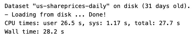

This code snippet demonstrates how to use the SimFin library to load daily share price data for US stocks. Initially, the %time command, a special Jupyter Notebook command, is utilized to display the time taken to execute a particular cell. Subsequently, a StockHub object is created from the SimFin library, configured for the US market with a setting to refresh share prices every 100 days. Following this, the StockHub object uses the load_shareprices method, specifying the variant=’daily’ parameter to load the daily share price data for US stocks. This approach is practical for fetching and using financial data for analysis or research purposes. By employing SimFin, users gain access to a comprehensive range of financial data, including balance sheets, income statements, and share price data, which can be utilized for various financial analyses, modeling, and decision-making processes. Moreover, the %time magic command records the time taken to load this data, enabling users to monitor the performance of data loading operations efficiently.

Calculates valuation signals using financial data

%%time
# Calculate valuation signals such as P/Sales.
# Automatically downloads the required financial statements.
df_val_signals = hub.val_signals()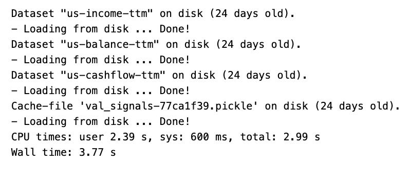

This code segment employs the val_signals() function from the hub module to calculate valuation signals like P/Sales using financial data automatically downloaded by the function. The %%time magic command is included to measure and display the execution time of this operation. The val_signals() function likely retrieves financial statement data, such as revenue and market capitalization, to calculate valuation metrics like the price-to-sales ratio. This process is automated and efficient, eliminating the need for manually gathering or processing the data. The result is a DataFrame (df_val_signals) that contains the calculated valuation signals for further analysis and decision-making. By using this code, time and effort are saved through the automation of fetching financial data and deriving valuation signals, thereby enabling quicker and more informed analysis and decision-making based on these metrics.

Prepare and clean daily stock data

# Use the daily "Total Return" series which is the stock-price
# adjusted for stock-splits and reinvestment of dividends.
# This is a Pandas DataFrame in matrix-form where the rows are
# time-steps and the columns are for the individual stock-tickers.
daily_prices = df_daily_prices[TOTAL_RETURN].unstack().T

# Remove rows that have very little data. Sometimes this dataset
# has "phantom" data-points for a few stocks e.g. on weekends.
num_stocks = len(daily_prices.columns)
daily_prices = daily_prices.dropna(thresh=int(0.1 * num_stocks))

# Remove the last row because sometimes it is incomplete.
daily_prices = daily_prices.iloc[0:-1]

# Show it.
daily_prices.head()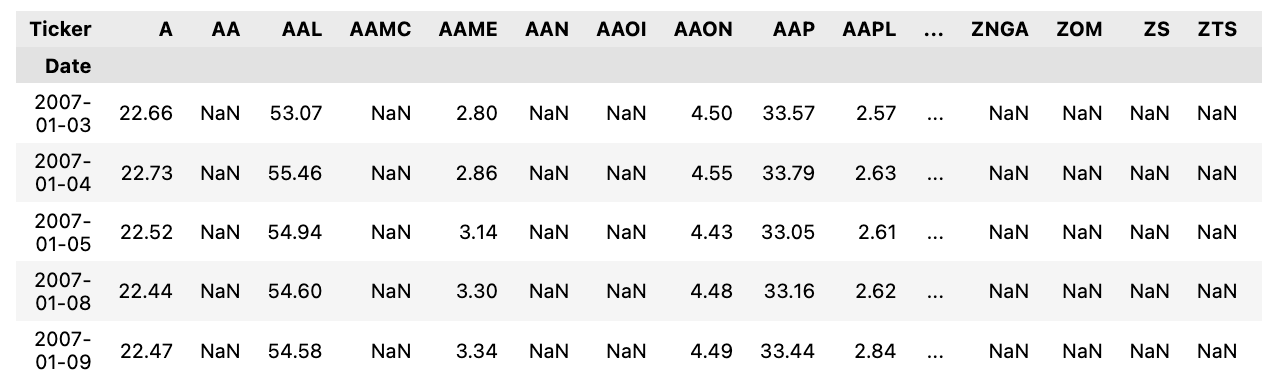

This code processes a pandas DataFrame representing daily stock prices in total return format. Initially, it extracts the Total Return series from the DataFrame, reshaping the data into a matrix where each row corresponds to a time-step and each column represents an individual stock ticker. Subsequently, it removes rows (time-steps) that contain insufficient data by dropping rows with NaN values in more than 10% of the columns. Additionally, it eliminates the last row, as this row may be incomplete due to the timing of data retrieval or recording. The end result is a cleaned and processed DataFrame of daily total return stock prices, ready for further analysis or visualization. This code is vital as it ensures the data is in the appropriate format for downstream analysis and excludes any incomplete or unreliable data points that might negatively impact the analysis.

Calculate daily stock returns from total returns

# Daily stock-returns calculated from the "Total Return".
# We could have used SimFin's function hub.returns() but
# this code makes it easier for you to use another data-source.
# This is a Pandas DataFrame in matrix-form where the rows are
# time-steps and the columns are for the individual tickers.
daily_returns_all = one_period_returns(prices=daily_prices, future=True)

# Remove empty rows (this should only be the first row).
daily_returns_all = daily_returns_all.dropna(how='all')

# Show it.
daily_returns_all.head()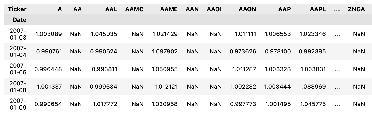

This code snippet calculates the daily stock returns from the Total Return data provided using a function named one_period_returns. This function computes the daily returns based on the given daily prices, with the parameter future=True indicating the calculation of returns from today to tomorrow. After the returns are calculated, the code removes any empty rows, primarily focusing on the first row, to clean up any invalid or incomplete data resulting from the calculations. The code then displays the first few rows of the DataFrame that contain the calculated daily returns for each ticker, with columns representing individual stocks and rows representing time steps. This process is useful because it converts the total return data into daily returns, facilitating easier analysis and comparison of different stocks’ performance on a daily basis. By providing daily return data, investors can gain a better understanding of the volatility and performance of individual stocks or their portfolio.

Retrieve list of all stock-tickers

# All available stock-tickers.
all_tickers = daily_prices.columns.to_list()

This code snippet extracts all the stock tickers from a DataFrame named daily_prices and stores them in a list named all_tickers. Stock tickers are unique symbols assigned to publicly traded companies for identification. The .columns attribute in pandas refers to the column labels in a DataFrame, and the .to_list() method converts these column labels into a Python list. This extraction is useful for obtaining a comprehensive list of all stock tickers present in a dataset or DataFrame. With all the tickers in a list, it becomes easier to iterate over them for further analysis, data manipulation, or visualization purposes.

Identify low median market-cap tickers

# Find tickers whose median daily trading market-cap < 1e6
daily_trade_mcap = df_daily_prices[CLOSE] * df_daily_prices[VOLUME]
mask = (daily_trade_mcap.median(level=0) < 1e7)
bad_tickers1 = mask[mask].reset_index()[TICKER].unique()

This code snippet filters out ticker symbols based on their median daily trading market capitalization being less than $1 million. First, it calculates the daily trading market capitalization for each ticker by multiplying the closing price and the trading volume from the provided DataFrame df_daily_prices. Next, it determines the median of these daily trading market capitalizations by grouping the values by ticker symbol and finding the median for each group.

Following this, the code creates a mask to identify tickers whose median daily trading market capitalization is less than $1 million. Then, using this mask, it filters out the ticker symbols that meet the condition and stores them in the bad_tickers1 variable. To avoid duplicates, it finally extracts unique ticker symbols from these filtered results.

This code is particularly useful in financial analysis or stock market studies to identify stocks with relatively smaller daily trading market capitalizations, providing a basis for further analysis or investment decisions. By identifying these bad tickers, one can refine investment choices or enhance risk assessment strategies.

Identifies volatile stocks with high returns

# Find tickers whose max daily returns > 100%
mask2 = (daily_returns_all > 2.0)
mask2 = (np.sum(mask2) >= 1)
bad_tickers2 = mask2[mask2].index.to_list()

This code snippet filters out tickers whose maximum daily returns exceed 100%. It achieves this by first creating a mask (mask2) that identifies tickers with daily returns greater than 2.0, equivalent to a 100% increase. It then checks if at least one ticker meets this condition by summing the True values in the mask. Finally, the code extracts the tickers that satisfy this criterion and stores them in a list called bad_tickers2.

This process proves useful in financial analysis or when dealing with stock market data, as it helps identify extreme price movements. By pinpointing tickers with maximum daily returns exceeding 100%, investors or analysts can investigate the reasons behind such movements and take appropriate actions, such as conducting detailed analyses, implementing risk management strategies, or making informed investment decisions.

Identify tickers with few data points

# Find tickers which have too little data, so that more than 20%
# of the rows are NaN (Not-a-Number).
mask3 = (daily_returns_all.isna().sum(axis=0) > 0.2 * len(daily_returns_all))
bad_tickers3 = mask3[mask3].index.to_list()

The provided code aims to identify and extract stock symbols (tickers) with a significant amount of missing data in a dataset. Specifically, it focuses on tickers with more than 20% missing values (NaN). The process begins by calculating the number of NaN values in each column of the daily_returns_all DataFrame using the expression daily_returns_all.isna().sum(axis=0). This computation results in a Series where the index corresponds to column names (tickers) and the values represent the count of NaN values in each column.

Next, the code checks if the count of NaN values exceeds 20% of the total number of rows in the DataFrame. This is achieved with the condition (daily_returns_all.isna().sum(axis=0) > 0.2 * len(daily_returns_all)). The outcome of this condition is a boolean Series (mask) indicating whether each ticker has more than 20% missing values.

Finally, the tickers satisfying this condition are extracted. The index values (tickers) where the condition is True are converted to a list, which is then assigned to the variable bad_tickers3. This code is crucial for data cleaning and analysis as it identifies tickers with insufficient data, thereby ensuring the quality and reliability of subsequent analyses.

Identifies delisted stocks ending with ‘_old’