Mastering Stock Market Predictions: Machine Learning, LSTM, and Statistical Analysis

In this article, we will delve into the cutting-edge techniques being used for stock market predictions.

From visually representing technical indicators to enhance our understanding of market behavior, to implementing machine learning projects specifically designed for stock market prediction, we leave no stone unturned. We will explore the application of Long Short-Term Memory (LSTM) networks, a type of recurrent neural network renowned for remembering past information, perfect for the temporal nature of stock market data.

# Import Modules

import numpy as np
import pandas as pd
import os
import random
import copy
import matplotlib.pyplot as plt
import pandas

You imported the following modules in your code snippet:

Python’s numpy library is used for scientific computations. In addition to arrays, matrices, and related routines, it contains a high-level interface to these objects.

Python’s pandas library is used to analyze data. Data structures and analysis tools are provided in an easy-to-use, high-performance package.

Operating system functions are provided by OS, which is a module.

The random module provides functions for generating random numbers.

The copy module provides functions for copying objects.

Python plots can be created using matplotlib.pyplot.

Python’s pandas library allows you to analyze data. A high-level data structure and data analysis tools are provided.

In the current namespace, a module is imported using the import statement. By using this approach, you don’t have to specify the full path to the module to use its functions and variables. To create an array, for instance, you can use the np.array() function after importing the numpy module.

Onepagecode’s Newsletter is a reader-supported publication. To receive new posts and support my work, consider becoming a free or paid subscriber.

Choose 8 random stock data for analysis

#filenames = [x for x in os.listdir("./Stocks/") if x.endswith('.txt') and os.path.getsize(x) > 0]
filenames = random.sample([x for x in os.listdir() if x.endswith('.txt') 
                           and os.path.getsize(os.path.join('',x)) > 0], 8)
print(filenames)

In the code snippet, a variable called filenames is defined and a list of file names is assigned to it. To find these file names, use the os.listdir() function to list all the files in the ./Stocks/ directory. File names ending in .txt and with a file size greater than 0 are included in the list. Due to the fact that it begins with a #, the line is currently commented out.

Following that, the code snippet assigns a list of 8 random file names to another variable called filenames. In the current directory (where the script is running), all files that end with .txt and have a file size greater than 0 are selected. We randomly select 8 file names from the list using random.sample().

Lastly, the code snippet prints the list of 8 randomly selected filenames.

The code retrieves a list of file names that meet certain criteria (ending with .txt and having a non-zero file size) from a specific directory or the current directory, and then selects 8 random file names from it. The selected file names are then printed.

Read data into dataframes

data = []
for filename in filenames:
    df = pd.read_csv(os.path.join('',filename), sep=',')
    label, _, _ = filename.split(sep='.')
    df['Label'] = label
    df['Date'] = pd.to_datetime(df['Date'])

    data.append(df)

Data is extracted from a collection of files using the provided code.

To store the data from the files, it first creates an empty list called “data”.

In the next step, it iterates over each file name listed in the “filenames” list.

Using the read_csv() function from the pandas library, it reads the contents of each file as a CSV file. To construct the full file path, the os.path.join() function joins an empty string with the current file name.

With the separator set to “….”, the file name is split using the split() function. This splits the file name into two parts, and the first part is assigned to the variable “label”. A “label” is a label or identifier that identifies the data in the file.

A new column named “Label” is added to the DataFrame (df) obtained from the file, and its values are set to the “label” variable. DataFrame rows are labelled accordingly in this column.

A new column, “Date”, is added to the DataFrame, and the existing “Date” column is converted to datetime using the pandas function pd.to_datetime().

Lastly, all DataFrames created from the files are added to the “data” list.

This code reads multiple files, extracts relevant data, assigns labels and converts dates to datetime format, and stores the resulting DataFrames in a list.

data[0].head()

Data[0].head() retrieves the first few rows of data from the DataFrame at index 0 of the “data” list.

What it does is as follows:

The element at index 0 of the “data” list is accessed by data[0]. DataFrames are contained in the “data” list, so data[0] refers to the first DataFrame.

A DataFrame can be called with .head(). The first few rows of the DataFrame are retrieved. The first five rows are returned by default.

The data[0].head() method retrieves the first 5 rows of data from the first DataFrame in the “data” list.

Add various Technical Indicators in the dataframe

def rsi(values):
    up = values[values>0].mean()
    down = -1*values[values<0].mean()
    return 100 * up / (up + down)

Your code defines a function called rsi that calculates the Relative Strength Index (RSI) based on a given set of parameters.

We can calculate the RSI for all input values by passing a single argument called values.

Following are the steps taken by the function:

Only values greater than zero are included in the values array. The mean (average) of these filtered values is assigned to the variable up. Values changed on average positively.

Only values less than zero are included in the values array. The mean (average) of these filtered values is calculated and assigned to the variable down. By multiplying it by -1, negative values become positive. The average negative change in values is shown here.

RSI is calculated by dividing average positive change (up) by average negative change (down). The result is then multiplied by 100 to get a percentage. RSI is an indicator used in technical analysis to assess the strength or weakness of a trend.

# Add Momentum_1D column for all 15 stocks.
# Momentum_1D = P(t) - P(t-1)
for stock in range(len(TechIndicator)):
    TechIndicator[stock]['Momentum_1D'] = (TechIndicator[stock]['Close']-TechIndicator[stock]['Close'].shift(1)).fillna(0)
    TechIndicator[stock]['RSI_14D'] = TechIndicator[stock]['Momentum_1D'].rolling(center=False, window=14).apply(rsi).fillna(0)
TechIndicator[0].tail(5)

A number of steps are performed by the provided code. Firstly, it adds two new columns, “Momentum_1D” and “RSI_14D,” to each DataFrame in the “TechIndicator” list. The one-day momentum indicator and the 14-day RSI indicator will be stored in these columns. Each DataFrame in the “TechIndicator” list is then iterated over and calculations are performed. It calculates one-day momentum by subtracting the previous day’s closing price from the current day’s closing price, and stores the result in the “Momentum_1D” column. This column is filled with 0 if there are any missing values. Furthermore, it calculates the 14-day RSI by applying a custom function called “rsi” to the values in the “Momentum_1D” column over a rolling window of size 14. In the “RSI_14D” column, the result is stored, and any missing values in this column are also filled with 0. In the “TechIndicator” list, the code prints the last 5 rows of data from the first DataFrame. This code adds and populates columns for momentum and RSI indicators for each stock’s closing price, providing additional insights.

for stock in range(len(TechIndicator)):
    TechIndicator[stock]['Volume_plain'] = TechIndicator[stock]['Volume'].fillna(0)
TechIndicator[0].tail()

Following are the steps performed by the code you provided:

The TechIndicator list is looped over using the stock variable in a for loop. TechIndicator list length is included in the loop.

A DataFrame at each index stock in the TechIndicator list is added to the loop as follows:

In the DataFrame, it creates a new column called Volume_plain.

Volume_plain contains the values from the Volume column, but any missing values (NaN) are replaced with 0.

By using the .tail() function, it prints the last 5 rows of data from the first DataFrame in the TechIndicator list (TechIndicator[0]).

A new column called Volume_plain is added to each DataFrame, and it is filled with Volume values, leaving any missing values as 0. The code iterates over the TechIndicator list. After that, it displays the last 5 rows of data from the first DataFrame in the TechIndicator list. By adding a new column and providing a summary view of the data, this code essentially modifies the DataFrames.

Onepagecode’s Newsletter is a reader-supported publication. To receive new posts and support my work, consider becoming a free or paid subscriber.

Calculation of Bollinger Bands

def bbands(price, length=30, numsd=2):
    """ returns average, upper band, and lower band"""
    #ave = pd.stats.moments.rolling_mean(price,length)
    ave = price.rolling(window = length, center = False).mean()
    #sd = pd.stats.moments.rolling_std(price,length)
    sd = price.rolling(window = length, center = False).std()
    upband = ave + (sd*numsd)
    dnband = ave - (sd*numsd)
    return np.round(ave,3), np.round(upband,3), np.round(dnband,3)

Your code defines a function called “bbands” that calculates Bollinger Bands for a given price series.

What it does is as follows:

Bollinger Bands can be calculated using three arguments: “price” (the price series), “length” (the window length for calculating the average and standard deviation), and “numsd” (the number of standard deviations to use for calculating the upper and lower bands).

The docstring indicates that the function returns the average, upper band, and lower band.

Using price.rolling(window=length, center=False).mean(), the code calculates the rolling average (mean) of the price series and assigns it to the variable “ave”. In the price series, this calculates the average value for each window of length “length”.

Using price.rolling(window=length, center=False).std(), it calculates the rolling standard deviation of the price series and assigns it to the variable “sd”. In this example, we calculate the standard deviation for each window of length “length” in the price series.

The upper band is calculated by adding “numsd” times the standard deviation to the average: ave + (sd * numsd). Bollinger Bands’ upper boundary is represented by this line.

A lower band is calculated by subtracting “numsd” times the standard deviation from the average: ave — (sd * numsd). Bollinger Bands’ lower boundary is represented by this line.

As a final step, it returns the average, upper band, and lower band as tuples, each rounded to three decimal places using np.round().

In summary, the code calculates Bollinger Bands based on a price series. Upper and lower bands are calculated using the rolling average and standard deviation, and the average, upper band, and lower band are returned rounded. An overbought or oversold condition in financial markets can be identified using Bollinger Bands, a popular technical analysis tool.

for stock in range(len(TechIndicator)):
    TechIndicator[stock]['BB_Middle_Band'], TechIndicator[stock]['BB_Upper_Band'], TechIndicator[stock]['BB_Lower_Band'] = bbands(TechIndicator[stock]['Close'], length=20, numsd=1)
    TechIndicator[stock]['BB_Middle_Band'] = TechIndicator[stock]['BB_Middle_Band'].fillna(0)
    TechIndicator[stock]['BB_Upper_Band'] = TechIndicator[stock]['BB_Upper_Band'].fillna(0)
    TechIndicator[stock]['BB_Lower_Band'] = TechIndicator[stock]['BB_Lower_Band'].fillna(0)
TechIndicator[0].tail()

In a for loop with the variable “stock”, it iterates over the range of numbers from 0 to the length of the “TechIndicator” list. Using this loop, we can operate on each stock on the “TechIndicator” list.

Using the “TechIndicator” loop, for each stock at index “stock”:

The function “bbands” calculates Bollinger Bands for the stock’s closing prices (“TechIndicator[stock][‘Close’]”) with a length of 20 and a standard deviation of 1. In the DataFrame of the current stock, three new columns are created: “BB_Middle_Band,” “BB_Upper_Band,” and “BB_Lower_Band.”.

With .fillna(0), it fills any missing values (NaNs) in the “BB_Middle_Band,” “BB_Upper_Band,” and “BB_Lower_Band” columns with 0.

Using the .tail() function, it prints the last few rows of data from the first DataFrame in the “TechIndicator” list (TechIndicator[0]).

For each stock in the “TechIndicator” list, Bollinger Bands are calculated and added. As it iterates through each stock, it calls the “bbands” function to calculate Bollinger Bands based on its closing price, and stores the results in new columns. A value of 0 is substituted for any missing values in the Bollinger Bands columns. Following that, the code prints the last few rows of data for the first stock on the “TechIndicator” list.

Calculation of Aroon Oscillator

def aroon(df, tf=25):
    aroonup = []
    aroondown = []
    x = tf
    while x< len(df['Date']):
        aroon_up = ((df['High'][x-tf:x].tolist().index(max(df['High'][x-tf:x])))/float(tf))*100
        aroon_down = ((df['Low'][x-tf:x].tolist().index(min(df['Low'][x-tf:x])))/float(tf))*100
        aroonup.append(aroon_up)
        aroondown.append(aroon_down)
        x+=1
    return aroonup, aroondown

This code introduces a function named “aroon” which computes the Aroon indicators for a DataFrame that contains financial data. Indicators help analyze the strength and direction of trends in financial markets.

In order to calculate the Aroon indicators, the function requires two arguments: the DataFrame containing the financial data and the time period (with a default value of 25).

The function initializes two empty lists, “aroonup” and “aroondown.” The values computed by this function will be stored in these lists.

Iterating through the DataFrame while calculating the Aroon indicators requires the variable named “x” to be set to the value of “tf.” The while loop continues until “x” reaches the length of the ‘Date’ column in the DataFrame. In this way, data ranges are taken into account when performing calculations.

In each iteration of the loop, the Aroon Up value is computed by finding the index of the highest value in the ‘High’ column within the previous “tf” number of periods. A percentage value is calculated by dividing this index by “tf” and multiplying it by 100.

Similarly, the Aroon Down value is calculated based on the lowest value in the ‘Low’ column over the previous “tf” period. Additionally, this index is divided by “tf” and multiplied by 100.

Calculated Aroon Up and Aroon Down values are appended to the “aroonup” and “aroondown” lists, respectively. The variable “x” is incremented after each iteration, enabling the loop to progress to the next period.Finally, the function returns the lists “aroonup” and “aroondown,” which contain the computed Aroon Up and Aroon Down values.

A given DataFrame of financial data is used to calculate Aroon indicators in the provided code. Each time the DataFrame is iterated over, the Aroon Up and Aroon Down values are computed, and separate lists are produced for each period. By returning these lists, the function is able to assess the strength and direction of financial markets’ trends.

for stock in range(len(TechIndicator)):
    listofzeros = [0] * 25
    up, down = aroon(TechIndicator[stock])
    aroon_list = [x - y for x, y in zip(up,down)]
    if len(aroon_list)==0:
        aroon_list = [0] * TechIndicator[stock].shape[0]
        TechIndicator[stock]['Aroon_Oscillator'] = aroon_list
    else:
        TechIndicator[stock]['Aroon_Oscillator'] = listofzeros+aroon_list

The code calculates and assigns Aroon Oscillator values for each stock in the “TechIndicator” list. Its functionality is as follows:

The code initiates a for loop that loops through the range of numbers from 0 to the length of the “TechIndicator” list. The following steps can be performed individually on each stock using this loop.

In the loop, for each stock in the “TechIndicator” list at the current index “stock”:

A list of 25 zeros is created, named “listofzeros”. The code will use this list later.

As an argument, the current stock’s data is passed to the function “aroon”. Assigned to the variables “up” and “down”, this function calculates the Aroon Up and Aroon Down values specific to the stock.

By using a list comprehension, we create a new list called “aroon_list”. The Aroon Oscillator values are calculated by subtracting the corresponding elements in the “up” and “down” lists.

A check is then made to determine if “aroon_list” has a length of zero. Then the stock has no Aroon values. This creates a new list consisting of zeros with the same length as the stock’s data (TechIndicator[stock]). The new list is assigned to “aroon_list”.

Alternatively, if “aroon_list” is not zero, Aroon values have been calculated successfully. The code proceeds to the next step without modifying “aroon_list”.

Lastly, the code assigns the values of “aroon_list” to a new column called “Aroon_Oscillator” in the DataFrame specific to the current stock (TechIndicator[stock]). Using list concatenation, if “aroon_list” is not empty, its values are appended to the beginning of “listofzeros”. “Aroon_Oscillator” is assigned the values of “aroon_list” if “aroon_list” is empty, meaning no Aroon values were calculated.

Calculation of Price Volume Trend

for stock in range(len(TechIndicator)):
    TechIndicator[stock]["PVT"] = (TechIndicator[stock]['Momentum_1D']/ TechIndicator[stock]['Close'].shift(1))*TechIndicator[stock]['Volume']
    TechIndicator[stock]["PVT"] = TechIndicator[stock]["PVT"]-TechIndicator[stock]["PVT"].shift(1)
    TechIndicator[stock]["PVT"] = TechIndicator[stock]["PVT"].fillna(0)
TechIndicator[0].tail()

The code calculates and populates the Price Volume Trend (PVT) values for each stock in the “TechIndicator” list. The following are some of its features:

A for loop is used to iterate through the range of numbers from 0 to the length of the “TechIndicator” list. Using this loop, each stock can be processed individually.

For each stock in the current index “stock” of the “TechIndicator” list:

In the DataFrame, a new column called “PVT” is created. Calculated PVT values will be stored in this column.

In order to calculate the PVT value, we divide the one-day momentum (“Momentum_1D”) by the previous day’s closing price (“Close” column at time t-1). Multiply the result by the current trading volume (“Volume”). The purpose of this calculation is to assess the relationship between price changes and trading volume.

By subtracting the obtained PVT value from the previous day’s PVT value, the change in PVT is determined. Tracking PVT trends over time is enabled by this step.

Using the .fillna(0) function, any missing values (NaNs) are filled with 0. By doing so, all data points are represented numerically in the column.

The code prints the last few rows of data from the first DataFrame in the “TechIndicator” list (TechIndicator[0]) using the .tail() function. As a result, we can see the PVT values for the first stock.

Overall, the code calculates and adds the Price Volume Trend (PVT) values to the DataFrames of each stock in the “TechIndicator” list. In order to calculate PVT values, the one-day momentum, previous closing prices, and trading volume are taken into account. If any values are missing, they are filled with 0. In the DataFrame for the first stock, the code displays the last few rows of PVT data. In financial analysis, PVT is used to analyze the interaction between price movements and trading volumes.

Calculation of Acceleration Bands

def abands(df):
    #df['AB_Middle_Band'] = pd.rolling_mean(df['Close'], 20)
    df['AB_Middle_Band'] = df['Close'].rolling(window = 20, center=False).mean()
    # High * ( 1 + 4 * (High - Low) / (High + Low))
    df['aupband'] = df['High'] * (1 + 4 * (df['High']-df['Low'])/(df['High']+df['Low']))
    df['AB_Upper_Band'] = df['aupband'].rolling(window=20, center=False).mean()
    # Low *(1 - 4 * (High - Low)/ (High + Low))
    df['adownband'] = df['Low'] * (1 - 4 * (df['High']-df['Low'])/(df['High']+df['Low']))
    df['AB_Lower_Band'] = df['adownband'].rolling(window=20, center=False).mean()

his code accomplishes the following:

DataFrame containing financial data is represented by the argument “df” in the function.

The first thing it does is introduce a new column in the DataFrame called “AB_Middle_Band.” This column’s values are determined by computing the rolling mean (average) of the “Close” column over a window of 20 periods. Using .rolling(window=20, center=False).mean() simplifies this calculation.

The code calculates the upper band values by multiplying the values in the “High” column by a factor derived from the difference between the corresponding values in the “High” and “Low” columns. A one-time increment is applied to the multiplication factor. A column called “aupband” contains the computed values.

By using the .rolling(window=20, center=False).mean() function, a new column titled “AB_Upper_Band” is created in the DataFrame. This column calculates the rolling mean using a window of 20 periods.

The code calculates the lower band values by multiplying the values in the “Low” column by the difference between the corresponding values in the “High” and “Low” columns. Subtracting this factor from 1 results in the multiplication factor. An “adownband” column is used to temporarily store the obtained values.

The DataFrame also includes a column named “AB_Lower_Band”. Using the .rolling(window=20, center=False).mean() function, this column calculates the rolling mean over a window of 20 periods.

Abands is a function defined in the provided code that calculates Acceleration Bands for a given DataFrame. In this function, three columns are added to the DataFrame: “AB_Middle_Band,” “AB_Upper_Band,” and “AB_Lower_Band.” The middle band represents the rolling average of the closing prices, while the upper and lower bands are determined by multiplying the high and low prices, respectively, with appropriate factors derived from their differences. A rolling mean calculation is used to smooth these bands’ values over a 20-period period. In technical analysis, acceleration bands are widely used to identify potential price levels and market trends.

for stock in range(len(TechIndicator)):
    abands(TechIndicator[stock])
    TechIndicator[stock] = TechIndicator[stock].fillna(0)
TechIndicator[0].tail()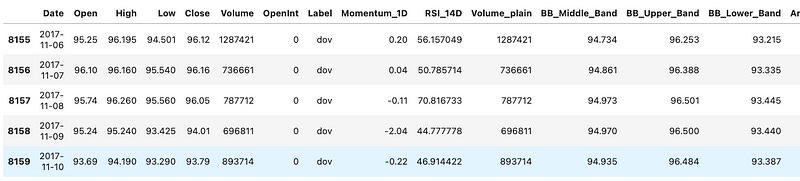

This code, the Acceleration Bands are calculated and processed for each stock on the “TechIndicator” list as follows: