Mastering Vectorized Backtesting in Algorithmic Trading

Part 4/10 In the realm of algorithmic trading and high-frequency market strategies, vectorized backtesting has emerged as a transformative approach that transcends traditional loop-based paradigms.

Read Part 1

Read Part 2

Read Part 3

As the complexity of modern financial markets increases and the volume of data swells, the ability to process large datasets in real time becomes a critical factor. This chapter delves into the advanced methodologies that underpin vectorized backtesting, providing a comprehensive exploration of the mathematical foundations, algorithmic innovations, and integration techniques necessary for developing sophisticated, production-grade trading systems.

At its core, vectorized backtesting harnesses the power of parallelized computations and advanced matrix operations to simulate trading strategies with minimal latency. Unlike conventional loop-based implementations that sequentially process data, vectorized techniques operate on entire arrays or matrices of data simultaneously. This shift not only enhances computational efficiency but also allows for a more nuanced exploration of intricate market behaviors and risk patterns. By building upon the foundational concepts of linear algebra, calculus, and probability theory, vectorized backtesting models can incorporate multifaceted decision rules and dynamic risk adjustments in a streamlined, computationally efficient manner.

Mathematical Underpinnings and Theoretical Optimization

Photo by Dan Cristian Pădureț on Unsplash

The theoretical framework of vectorized backtesting is rooted in advanced mathematics. The use of matrix algebra and vector calculus enables the representation of vast arrays of financial data in compact forms that are amenable to rapid manipulation. At the heart of these methodologies is the concept of tensor operations, which extend the ideas of matrices to higher-dimensional arrays. These operations allow for the simultaneous computation of multiple market variables, enabling traders to incorporate cross-asset correlations and multidimensional risk factors into their models.

In developing these advanced techniques, one must consider the optimization of computational resources. Mathematical optimization theories, such as convex optimization and gradient descent methods, provide a rigorous basis for refining trading strategies. In vectorized environments, the simultaneous adjustment of portfolio weights, risk exposure, and trading signals can be achieved by solving large-scale optimization problems where the objective functions are often non-linear and non-convex. Advanced solvers, which incorporate regularization techniques and stochastic approximations, are crucial for ensuring that the backtesting framework remains robust under varying market conditions.

A critical aspect of these optimization techniques involves the evaluation of performance metrics under different market scenarios. The integration of risk metrics, such as Value at Risk (VaR) and Conditional Value at Risk (CVaR), into the optimization process ensures that the backtesting framework not only maximizes returns but also accounts for tail risk and volatility clustering. The interplay between these mathematical constructs and vectorized operations allows for the rapid simulation of a myriad of market scenarios, thereby providing traders with a comprehensive understanding of strategy performance across different market regimes.

Mathematically, one can represent a trading strategy as a function that maps a high-dimensional state vector — comprising market indicators, asset prices, and risk parameters — to a trading decision. The backtesting process, in turn, involves applying this function across a time series of such vectors in a vectorized manner. This approach leads to the formulation of complex differential equations and recursive algorithms that capture the evolution of market dynamics and the resulting impact on portfolio performance. The challenge lies in efficiently solving these equations while maintaining numerical stability and ensuring that the solution converges to a realistic representation of market behavior.

In practice, these mathematical principles are embodied in a series of advanced functions that implement risk-adjusted performance metrics and dynamic allocation strategies. For instance, consider the following function definition that encapsulates a complex market impact model. The function employs a series of iterative refinements and non-linear adjustments to accurately simulate the decay factors associated with large orders:

def optimize_market_impact_calculation(order_book, trade_size, decay_factors, tolerance=1e-6, max_iterations=1000):
    """
    Perform an advanced optimization to calculate the market impact of a trade.
    This function uses iterative refinement to simulate non-linear decay effects
    associated with large order executions. The decay_factors parameter is a dictionary
    that specifies the decay rate for each level of the order book.
    
    Parameters:
        order_book: A high-dimensional list representing market depth.
        trade_size: The volume of the trade for which the impact is calculated.
        decay_factors: A dictionary mapping each order book level to its decay rate.
        tolerance: Convergence criteria for iterative refinement.
        max_iterations: Maximum iterations allowed before terminating the calculation.
    
    Returns:
        impact: The calculated market impact as a float.
    """
    impact = 0.0
    iteration = 0
    previous_impact = float('inf')
    
    while iteration < max_iterations and abs(previous_impact - impact) > tolerance:
        previous_impact = impact
        impact = 0.0
        for level, volume in enumerate(order_book):
            decay = decay_factors.get(level, 1)
            # Simulate non-linear decay: the impact is a function of trade size, volume, and decay factor.
            impact += (trade_size ** 0.5) * (volume ** 0.75) * decay
        # Apply an adjustment factor based on previous iterations to ensure convergence.
        impact = impact * 0.98 + previous_impact * 0.02
        iteration += 1
    
    return impact

This function epitomizes the blend of mathematical sophistication and algorithmic precision required in advanced vectorized backtesting frameworks. The iterative approach ensures that the function remains resilient to the complexities of real-world order book dynamics, while the non-linear decay computations capture the nuanced effects of large trade executions.

Algorithmic Innovations and Integration Techniques

Beyond the theoretical foundations, the practical application of vectorized backtesting necessitates innovative algorithmic strategies. Modern trading systems must integrate a multitude of signal-generating mechanisms, risk adjustment protocols, and execution models into a cohesive, highly optimized framework. Advanced algorithms are designed not only to evaluate historical data efficiently but also to adapt dynamically to emerging market trends and anomalies.

One of the key innovations in this space is the use of dynamic programming techniques that recursively break down complex strategy evaluations into manageable sub-problems. This method allows for the reuse of intermediate computations, significantly reducing the overall computational load. When implemented in a vectorized context, these dynamic programming algorithms benefit from parallel execution, enabling the rapid analysis of multiple market scenarios simultaneously.

Another frontier in algorithmic innovation involves the integration of stochastic models that account for market uncertainty and random fluctuations. Techniques such as Monte Carlo simulations and Markov Chain modeling are increasingly being adapted for vectorized environments. These methods allow traders to simulate thousands of potential market paths in parallel, providing a probabilistic assessment of strategy performance and risk exposure. By incorporating these stochastic elements into vectorized backtesting frameworks, developers can better understand the distribution of potential outcomes and refine their strategies to mitigate adverse events.

Algorithmic innovations are also reflected in the evolution of execution logic. Traditional rule-based systems are gradually being supplanted by adaptive algorithms that leverage machine learning techniques. These models, trained on historical market data, can identify subtle patterns and adjust trading parameters in real time. The integration of neural network architectures, such as convolutional or recurrent networks, with vectorized computations allows for the extraction of high-level features from raw market data, enabling more precise predictions of market movements. The transition from static to dynamic models represents a paradigm shift in backtesting methodologies, as strategies are no longer confined to pre-defined rules but can evolve in response to market conditions.

To illustrate these advanced algorithmic techniques, consider a function definition that embodies a dynamic allocation strategy based on a neural-inspired architecture. The function iteratively refines its allocation decisions using a combination of gradient-based adjustments and historical performance feedback:

def dynamic_allocation_strategy(market_data, current_allocation, learning_rate, iterations=500):
    """
    Execute a dynamic allocation strategy that adjusts portfolio weights
    based on high-dimensional market data and performance feedback.
    The algorithm uses gradient-based refinements and recursive adjustment
    to optimize the allocation over a specified number of iterations.
    
    Parameters:
        market_data: A multidimensional array representing historical market signals.
        current_allocation: An initial vector of portfolio weights.
        learning_rate: A scalar that determines the magnitude of adjustments.
        iterations: The number of iterations to perform during optimization.
    
    Returns:
        optimized_allocation: The refined allocation vector after optimization.
    """
    optimized_allocation = current_allocation.copy()
    for iteration in range(iterations):
        gradient = [0] * len(optimized_allocation)
        # Compute gradient adjustments based on market performance and volatility.
        for i in range(len(optimized_allocation)):
            # Simulate a complex gradient calculation involving historical performance.
            gradient[i] = sum(market_data[j][i] * (optimized_allocation[i] - 0.5) for j in range(len(market_data))) / len(market_data)
        # Update the allocation using the calculated gradient.
        optimized_allocation = [max(0, weight - learning_rate * grad) for weight, grad in zip(optimized_allocation, gradient)]
        # Normalize the allocation vector to maintain full investment.
        total = sum(optimized_allocation)
        optimized_allocation = [weight / total for weight in optimized_allocation]
    return optimized_allocation

In this example, the function encapsulates an iterative optimization process that continuously refines portfolio allocations. The gradient calculations are intentionally designed to capture non-linear dependencies and adapt to the evolving market landscape. Such an approach highlights the shift towards more intelligent, self-correcting trading systems where learning and adaptation are embedded within the core execution logic.

System Architecture for Scalable Backtesting

As trading strategies become increasingly sophisticated, the underlying system architecture must evolve to support high-speed data processing, memory management, and parallel computation. This chapter explores the architectural considerations essential for deploying vectorized backtesting systems at scale. The discussion encompasses both the theoretical design principles and practical implementation patterns that ensure the system can handle the high throughput and low latency required in modern trading environments.

A robust system architecture for vectorized backtesting is characterized by its ability to efficiently manage data flow, memory resources, and computational parallelism. The first challenge lies in designing a data pipeline that can ingest and preprocess massive amounts of historical market data without becoming a bottleneck. Memory management strategies must be optimized to store and retrieve data in formats that are conducive to vectorized operations. Techniques such as memory mapping, shared memory constructs, and cache optimization are essential for maintaining high performance when dealing with large datasets.

The architecture must also support parallel processing, which is a cornerstone of vectorized backtesting. By leveraging multi-core processors and distributed computing frameworks, the system can perform simultaneous computations across multiple dimensions of market data. This parallelism is not limited to the raw data processing stage but extends into the optimization and simulation phases, where each trading scenario or market condition can be evaluated independently. The challenge here is to design the system in such a way that it maximizes resource utilization while minimizing inter-process communication overhead.

Distributed computation architectures, in particular, introduce additional complexities. The system must ensure that data remains consistent across distributed nodes, and that any discrepancies in computation due to network latency or asynchronous processing do not compromise the integrity of the backtesting results. Advanced synchronization mechanisms and consensus algorithms are employed to manage these challenges, ensuring that the distributed system behaves as a coherent whole.

In this context, a layered architecture is often the most effective approach. At the lowest level, a high-performance data ingestion layer handles the retrieval and initial processing of raw market data. Above this, a vectorized computation layer performs the core backtesting operations, utilizing optimized mathematical libraries and parallel processing frameworks. The top layer is responsible for strategy optimization and risk analysis, integrating advanced machine learning algorithms and dynamic programming techniques. Each layer is designed to operate semi-independently, yet they are tightly coupled through well-defined interfaces that facilitate efficient data exchange and synchronization.

A key architectural challenge is the efficient management of computational resources. In vectorized backtesting, the memory footprint can be substantial, and the need for rapid access to large matrices and tensors demands careful consideration of both hardware and software design. Techniques such as just-in-time (JIT) compilation and hardware acceleration through graphics processing units (GPUs) are increasingly being integrated into backtesting systems. These methods allow for the offloading of intensive computations to specialized hardware, thereby freeing up central processing resources for other critical tasks.

Furthermore, system architecture must account for fault tolerance and scalability. In production environments, backtesting systems are often required to run continuously, processing new data as it becomes available. The architecture must be resilient to hardware failures, software glitches, and network interruptions. Redundancy, load balancing, and real-time monitoring are essential components of a robust system, ensuring that the backtesting process can recover gracefully from unexpected disruptions without compromising data integrity.

To illustrate these architectural principles, consider a function that encapsulates a critical component of the data synchronization logic. This function is designed to operate in a distributed environment, ensuring that disparate nodes maintain a consistent view of the backtesting state. The logic employs advanced algorithms for consensus and synchronization, making it a vital piece of the overall system architecture:

def synchronize_backtesting_state(distributed_state, local_update, consensus_threshold, max_sync_rounds=10):
    """
    Synchronize the state of the backtesting system across distributed nodes.
    This function employs a consensus-based mechanism to ensure that all nodes converge
    on a consistent state, despite potential network delays and asynchronous updates.
    The synchronization process iteratively refines the local state based on updates from
    other nodes until the consensus threshold is met or the maximum number of sync rounds is reached.
    
    Parameters:
        distributed_state: A data structure representing the shared state across nodes.
        local_update: The local modifications to the state that need to be synchronized.
        consensus_threshold: A parameter that determines the acceptable level of state divergence.
        max_sync_rounds: Maximum iterations for synchronization attempts.
    
    Returns:
        synchronized_state: The updated and synchronized state after convergence.
    """
    synchronized_state = local_update.copy()
    sync_round = 0
    while sync_round < max_sync_rounds:
        divergence = 0.0
        for node_state in distributed_state:
            # Calculate divergence using a complex metric that considers multiple state dimensions.
            divergence += sum(abs(synchronized_state[i] - node_state[i]) for i in range(len(synchronized_state)))
        divergence /= len(distributed_state)
        if divergence < consensus_threshold:
            break
        # Adjust the synchronized state towards the average state of all nodes.
        averaged_state = [0] * len(synchronized_state)
        for i in range(len(synchronized_state)):
            averaged_state[i] = sum(node_state[i] for node_state in distributed_state) / len(distributed_state)
        synchronized_state = [(synchronized_state[i] + averaged_state[i]) / 2 for i in range(len(synchronized_state))]
        sync_round += 1
    return synchronized_state

This function exemplifies the intricacies of maintaining consistency across a distributed backtesting environment. The synchronization mechanism employs iterative refinement and advanced consensus metrics, ensuring that the distributed system converges on a coherent state even in the face of network-induced variability. The careful calibration of parameters such as the consensus threshold and maximum synchronization rounds reflects the tradeoffs between speed and precision that are inherent in such systems.

Performance Tuning, Tradeoffs, and Advanced Risk Management

In highly competitive financial markets, the performance of backtesting systems is as crucial as the accuracy of the underlying trading algorithms. This chapter examines the performance tuning techniques and optimization tradeoffs that are central to the development of advanced vectorized backtesting systems. It further explores the integration of sophisticated risk management protocols that ensure the robustness and resilience of trading strategies under volatile market conditions.

Performance tuning in vectorized backtesting is a multifaceted challenge that involves both algorithmic and architectural optimizations. At the algorithmic level, the focus is on minimizing computational overhead while maximizing the accuracy and speed of simulations. Techniques such as loop unrolling, memory prefetching, and vectorized operations are employed to ensure that each operation is executed as efficiently as possible. The use of just-in-time compilation and hardware-specific optimizations, particularly on GPUs and multi-core processors, allows for significant reductions in execution time, enabling the rapid processing of complex strategies and large datasets.

At the architectural level, performance tuning revolves around the efficient allocation of computational resources and the minimization of latency. This involves optimizing data storage formats, leveraging in-memory databases, and employing asynchronous processing models that decouple data ingestion from computation. The design of efficient data pipelines is paramount, as the ability to stream large volumes of market data directly into the computation engine without intermediate bottlenecks can have a profound impact on overall system performance.

The tradeoffs in performance tuning are often non-trivial. For instance, aggressive optimization may lead to code that is difficult to maintain and extend, while overly generic solutions may fail to fully exploit the capabilities of modern hardware. Developers must balance the need for speed with the necessity for code clarity and maintainability, particularly in systems that are expected to operate continuously in production environments. In many cases, performance tuning involves iterative profiling and benchmarking, where the system is subjected to a battery of tests under various load conditions. The insights gained from these tests guide the refinement of both algorithmic and architectural components, ensuring that the system remains robust and efficient as it scales.

Risk management is another critical aspect of advanced vectorized backtesting. The inherent uncertainty and volatility of financial markets necessitate the integration of dynamic risk assessment protocols into the backtesting process. Advanced risk management systems are designed to evaluate the potential impact of adverse market movements and to adjust trading strategies in real time. These systems often incorporate probabilistic models that estimate the likelihood of extreme events and employ stress-testing techniques to evaluate strategy performance under worst-case scenarios.

One of the key challenges in risk management is the avoidance of overfitting — a phenomenon where a strategy performs exceptionally well on historical data but fails to generalize to live market conditions. Advanced backtesting systems mitigate this risk by incorporating cross-validation techniques, out-of-sample testing, and the use of regularization methods within optimization algorithms. By dynamically adjusting model parameters based on real-time performance feedback, these systems maintain a delicate balance between exploiting historical trends and adapting to new market conditions.

The integration of performance metrics with risk management protocols allows for a holistic evaluation of trading strategies. Metrics such as Sharpe ratios, maximum drawdown, and risk-adjusted returns are computed using vectorized operations that provide rapid, high-fidelity insights into strategy performance. The seamless interplay between performance optimization and risk management not only enhances the reliability of backtesting outcomes but also empowers traders to make informed decisions in live trading environments.

An illustrative example of advanced performance tuning can be seen in the following function, which integrates risk assessment into the optimization process. This function encapsulates a complex algorithm that adjusts trading signals based on both performance metrics and risk thresholds:

def optimize_trading_signal(performance_history, risk_threshold, adjustment_factor, iterations=100):
    """
    Optimize the trading signal by integrating historical performance metrics with dynamic risk assessments.
    The function iteratively adjusts the trading signal based on a composite metric that accounts for both
    performance improvements and risk thresholds. The algorithm uses a gradient-inspired approach to converge
    on an optimal signal configuration.
    
    Parameters:
        performance_history: A multidimensional array representing historical performance metrics.
        risk_threshold: A scalar representing the maximum acceptable risk level.
        adjustment_factor: A factor used to scale the adjustments made to the trading signal.
        iterations: The number of iterations to perform during the optimization process.
    
    Returns:
        optimized_signal: The refined trading signal after the optimization process.
    """
    optimized_signal = [0.5 for _ in range(len(performance_history[0]))]
    for iteration in range(iterations):
        composite_metric = [0] * len(optimized_signal)
        for i in range(len(optimized_signal)):
            performance_metric = sum(performance_history[j][i] for j in range(len(performance_history))) / len(performance_history)
            # Adjust based on risk: if the performance metric exceeds the risk threshold, reduce the signal intensity.
            risk_adjustment = adjustment_factor if performance_metric > risk_threshold else -adjustment_factor
            composite_metric[i] = performance_metric + risk_adjustment
        optimized_signal = [max(0, min(1, optimized_signal[i] + 0.01 * composite_metric[i])) for i in range(len(optimized_signal))]
    return optimized_signal

This function demonstrates a sophisticated approach to integrating risk management directly into the signal optimization process. By evaluating historical performance in tandem with risk metrics, the algorithm ensures that trading signals are not only optimized for returns but also constrained within acceptable risk limits. The iterative, gradient-inspired refinement process reflects the advanced computational techniques that are emblematic of modern vectorized backtesting systems.

Complex Implementation Patterns and Integrative Analysis

As the sophistication of vectorized backtesting systems increases, so does the need for complex implementation patterns that can seamlessly integrate disparate components into a unified framework. In this chapter, we explore advanced integration strategies that bring together mathematical optimization, dynamic programming, parallel processing, and risk management into a cohesive whole. The discussion focuses on the challenges of combining these components in a manner that maximizes performance without sacrificing the flexibility and adaptability of the system.

The development of a complex backtesting framework often involves the orchestration of multiple subsystems, each responsible for a specific aspect of the overall strategy evaluation. For example, one subsystem might handle the ingestion and preprocessing of high-frequency market data, while another is dedicated to the vectorized computation of trading signals. Yet another component may focus on risk assessment and the dynamic adjustment of strategy parameters. The key to successful integration lies in the careful design of interfaces that allow these subsystems to communicate efficiently and effectively.

One of the most challenging aspects of integration is ensuring that the system can scale horizontally as data volumes increase and computational demands grow. This necessitates the use of modular design principles, where each component is encapsulated in a well-defined interface that abstracts away its internal complexities. Such an approach not only simplifies the integration process but also facilitates future upgrades and the incorporation of new algorithms. The emphasis is on building a system that is both resilient and adaptable, capable of incorporating emerging technologies and methodologies as they become available.

The integrative analysis of market data is another area where advanced implementation patterns come to the fore. Modern backtesting systems must be capable of synthesizing information from multiple sources, each with its own data structure, latency profile, and reliability metrics. This necessitates the development of sophisticated data fusion techniques that can reconcile these differences and produce a coherent view of market dynamics. Techniques such as Kalman filtering, Bayesian inference, and ensemble learning are increasingly being employed to merge diverse data streams into a unified analytical framework. The result is a system that can dynamically adjust its strategy in response to a comprehensive, real-time assessment of market conditions.

In addition to data fusion, the integration of real-time monitoring and alerting systems is crucial for ensuring the operational integrity of backtesting frameworks. As strategies are continuously optimized and executed, the system must be capable of detecting anomalies, identifying performance degradation, and initiating corrective actions autonomously. Advanced diagnostic algorithms, coupled with machine learning-based anomaly detection, enable the system to maintain a high level of reliability and performance even under adverse market conditions.

A prime example of an integrative implementation pattern is illustrated in the following function definition. This function represents a complex class that encapsulates the core components of a vectorized backtesting system, integrating dynamic programming, risk management, and performance optimization into a single coherent module:

class AdvancedBacktester:
    """
    A comprehensive class that encapsulates the advanced components of a vectorized backtesting system.
    This class integrates dynamic programming for signal optimization, risk management for real-time adjustment,
    and performance tuning for high-throughput computation. The design emphasizes modularity, scalability, and resilience.
    """
    
    def __init__(self, initial_state, risk_parameters, optimization_parameters):
        self.state = initial_state
        self.risk_parameters = risk_parameters
        self.optimization_parameters = optimization_parameters
        self.performance_metrics = {}
    
    def dynamic_signal_update(self, market_snapshot, iterations=200):
        """
        Update trading signals using dynamic programming and iterative optimization.
        This method refines the trading signal based on the current market snapshot,
        incorporating risk adjustments and performance feedback into the update mechanism.
        """
        signal = [0.5 for _ in range(len(market_snapshot))]
        for _ in range(iterations):
            gradient = [0] * len(signal)
            for i in range(len(signal)):
                # Advanced gradient calculation incorporating market snapshot and risk parameters.
                gradient[i] = sum(market_snapshot[j][i] * (signal[i] - self.risk_parameters.get('baseline', 0.5))
                                  for j in range(len(market_snapshot))) / len(market_snapshot)
            signal = [max(0, min(1, signal[i] - self.optimization_parameters.get('step_size', 0.01) * gradient[i]))
                      for i in range(len(signal))]
        self.state['signal'] = signal
        return signal
    
    def update_risk_metrics(self, performance_data):
        """
        Update the system's risk metrics based on recent performance data.
        This method calculates advanced risk measures such as dynamic VaR and volatility clustering
        using vectorized computations.
        """
        dynamic_var = sum(performance_data) / len(performance_data) * self.risk_parameters.get('multiplier', 1.5)
        self.state['risk'] = dynamic_var
        return dynamic_var
    
    def run_backtest_cycle(self, market_data_snapshot):
        """
        Execute a complete backtest cycle by integrating dynamic signal updates, risk metric adjustments,
        and performance evaluations. This method orchestrates the execution of the various components
        in a synchronized manner to produce a comprehensive simulation outcome.
        """
        signal = self.dynamic_signal_update(market_data_snapshot)
        risk = self.update_risk_metrics([sum(row) / len(row) for row in market_data_snapshot])
        self.performance_metrics['cycle'] = {'signal': signal, 'risk': risk}
        return self.performance_metrics['cycle']

This class demonstrates a high level of integration, where dynamic signal updates, risk metric recalibration, and performance tracking are seamlessly combined. The modular nature of the implementation allows for individual components to be fine-tuned without disrupting the overall system, and the use of iterative, gradient-based methods ensures that the backtesting process adapts in real time to evolving market conditions.

In addition to the internal logic encapsulated within the class, the broader implementation pattern involves a tightly coupled orchestration layer that manages data flows and synchronizes computations across distributed nodes. The integrative approach ensures that the system is capable of handling both batch processing of historical data and real-time adjustments in live trading environments. By abstracting away the complexities of data management and computational synchronization, the integrative analysis layer empowers developers to focus on refining the core trading algorithms and risk models.

Future Directions and Research Challenges in Vectorized Backtesting

Looking forward, the field of vectorized backtesting is poised for continued evolution, driven by advances in computational hardware, algorithmic innovation, and the growing complexity of financial markets. As the industry moves toward increasingly automated and adaptive trading systems, several research challenges and future directions emerge as critical areas for exploration.

One of the most promising directions is the integration of real-time machine learning models that not only predict market trends but also continuously update and refine trading strategies based on live data. The convergence of artificial intelligence with vectorized computation opens up avenues for developing systems that learn from every trade, adjusting their models on the fly to improve accuracy and reduce risk. These adaptive systems can incorporate reinforcement learning algorithms that evaluate the outcomes of trading decisions and adjust the strategy parameters accordingly, leading to a virtuous cycle of continuous improvement.

Another significant research challenge is the development of hybrid models that seamlessly integrate deterministic and stochastic approaches. In traditional backtesting, deterministic models provide clear, rule-based strategies that are easy to understand and implement. However, they often fall short in capturing the inherent uncertainty of financial markets. By blending deterministic models with stochastic simulations, researchers can develop hybrid systems that combine the clarity of rule-based approaches with the flexibility of probabilistic methods. This integration allows for a more realistic simulation of market behavior, where random fluctuations and systemic shocks are taken into account in a unified framework.

The increasing availability of high-frequency data also presents new opportunities and challenges for vectorized backtesting systems. As market participants generate vast quantities of data at sub-second intervals, the need for ultra-low latency processing becomes paramount. Future research will likely focus on the development of specialized hardware accelerators, such as field-programmable gate arrays (FPGAs) and application-specific integrated circuits (ASICs), that are tailored for the specific computational patterns of vectorized backtesting. These hardware innovations promise to deliver unprecedented processing speeds, enabling the real-time execution of even the most complex trading strategies.

In parallel with hardware advancements, the evolution of software paradigms will play a critical role in shaping the future of backtesting systems. The adoption of functional programming techniques, coupled with advanced concurrency models, is likely to yield systems that are both more resilient and easier to scale. Functional programming languages, with their emphasis on immutability and stateless computation, naturally lend themselves to the parallel processing patterns required for high-performance backtesting. The shift toward these paradigms will require a rethinking of existing algorithms and data structures, but the potential benefits in terms of speed, scalability, and maintainability are considerable.

The integration of regulatory and compliance considerations into backtesting frameworks represents yet another frontier for future research. As regulatory bodies demand greater transparency and accountability in algorithmic trading, backtesting systems must evolve to provide detailed audit trails and robust validation mechanisms. Advanced logging, provenance tracking, and automated compliance checks will become integral components of backtesting systems, ensuring that strategies not only perform well but also adhere to stringent regulatory standards. This integration of compliance features with performance optimization and risk management is a complex challenge that will require interdisciplinary collaboration between technologists, financial experts, and regulatory authorities.

A final area of research that holds significant promise is the development of self-healing and fault-tolerant backtesting systems. In a production environment, the ability to automatically detect and recover from errors is crucial for maintaining continuous operation. Future systems may incorporate advanced monitoring and diagnostic tools that leverage machine learning to predict and preemptively address potential failures. The concept of self-healing architectures, where the system autonomously reconfigures itself in response to anomalies, represents the cutting edge of distributed computing and is likely to play a pivotal role in the next generation of vectorized backtesting systems.

In conclusion, the evolution of vectorized backtesting is characterized by a relentless pursuit of efficiency, accuracy, and adaptability. From the rigorous mathematical foundations that underpin high-speed computations to the innovative algorithmic strategies that drive dynamic portfolio optimization, the field continues to push the boundaries of what is possible in algorithmic trading. The integration of advanced system architectures, sophisticated risk management protocols, and future-facing research initiatives promises to usher in an era of trading systems that are not only faster and more efficient but also more intelligent and resilient.

As researchers and practitioners continue to explore these frontiers, the interplay between theory and practice will remain a central theme. The challenges of scaling computations, managing complex data pipelines, and integrating diverse algorithmic paradigms require a holistic approach that marries deep technical expertise with a forward-thinking vision. The insights gleaned from advanced vectorized backtesting will undoubtedly shape the future of algorithmic trading, driving innovation across both the technological and financial domains.

Ultimately, the journey toward more sophisticated and robust backtesting systems is a testament to the power of interdisciplinary collaboration. It is a field where mathematics, computer science, finance, and engineering converge to create solutions that not only meet the demands of today’s markets but also anticipate the challenges of tomorrow. As we look to the future, the continued evolution of vectorized backtesting will serve as a catalyst for innovation, unlocking new opportunities and transforming the landscape of algorithmic trading.

Through this comprehensive exploration of advanced vectorized backtesting, we have highlighted the intricate balance between performance optimization, risk management, and system architecture. By delving into the mathematical foundations, examining complex integration patterns, and considering the future directions of this rapidly evolving field, we hope to have provided a robust framework for both researchers and practitioners. The road ahead is filled with challenges, but also with immense opportunities for those who dare to push the limits of what is possible in algorithmic trading.

The advanced techniques discussed herein not only build upon established practices but also chart new territory in the quest for ever more efficient and resilient trading systems. With a focus on rigorous mathematical analysis, sophisticated algorithm design, and innovative system integration, the next generation of vectorized backtesting promises to redefine the standards of performance and reliability in the fast-paced world of financial markets.

By embracing these advanced concepts and integrating them into real-world applications, developers and traders alike can harness the full potential of vectorized backtesting, paving the way for strategies that are both adaptive and predictive. This evolution will ultimately contribute to a more stable and efficient trading ecosystem, where technological innovation and financial acumen work in tandem to achieve unprecedented levels of performance and risk mitigation.

The advanced methodologies detailed in this chapter represent just one step in an ongoing journey — a journey defined by constant innovation, relentless optimization, and a deep commitment to excellence in the field of algorithmic trading. As new technologies emerge and markets continue to evolve, the principles of vectorized backtesting will remain at the forefront, guiding the development of systems that are not only state-of-the-art but also fundamentally transformative in their approach to simulating and executing trading strategies.

In the coming years, it is likely that the integration of real-time data analytics, advanced machine learning, and distributed computing will lead to even more sophisticated backtesting frameworks. These frameworks will be capable of processing vast amounts of information with unprecedented speed and accuracy, ultimately leading to a paradigm shift in how trading strategies are developed, tested, and deployed. The fusion of cutting-edge research and practical implementation will continue to drive the evolution of vectorized backtesting, ensuring that it remains a vital tool for navigating the complexities of modern financial markets.

---

The Need for Vectorized Backtesting

Vectorized backtesting leverages the power of array-based operations and parallel processing to bypass the inherent bottlenecks of iterative loops. The approach capitalizes on optimized, low-level libraries to perform operations on entire datasets concurrently, a process that is not only faster but also more scalable. The discussion that follows introduces advanced concepts that extend beyond basic loop-to-vector conversion, exploring dynamic function generation, adaptive optimization strategies, and integration techniques that coalesce to form a robust, production-grade backtesting framework.

Limitations of Loop-Based Backtesting

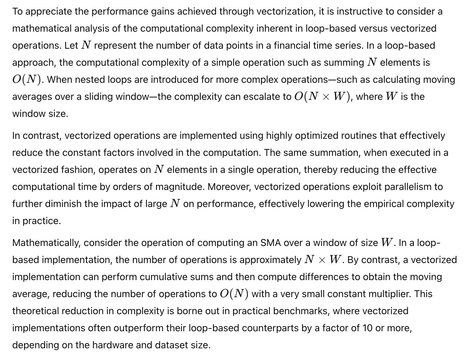
Traditional loop-based backtesting methods in languages like Python have long been plagued by significant computational overhead. In a loop-centric paradigm, each operation is executed sequentially, which magnifies the cumulative processing time when dealing with extensive datasets. The computational complexity grows linearly — or even exponentially in cases of nested loops — leading to prohibitive latency when simulating sophisticated trading strategies. This becomes particularly evident when executing tasks such as computing moving averages, volatility measures, or risk-adjusted returns across millions of data points.

Consider a scenario where a simple moving average (SMA) must be computed on a high-frequency dataset comprising millions of tick-level entries. In a loop-based implementation, each iteration must individually access and process elements of the dataset, incurring not only CPU cycle overhead but also frequent memory accesses that are far less efficient than block operations. Additionally, Python’s interpreter overhead in managing loop constructs further contributes to the overall delay, making real-time strategy validation and parameter optimization virtually infeasible.

The memory overhead in loop-based methods is equally problematic. Sequential processing of large arrays forces repeated context switches and often results in suboptimal caching behavior. In systems where the entire dataset cannot be held in cache, memory bandwidth becomes a critical bottleneck. Moreover, complex strategies involving nested loops exacerbate the situation by repeatedly recalculating intermediate results instead of exploiting temporal and spatial locality in memory.

Inefficiencies in High-Frequency Data Handling

Beyond sheer computational delays, loop-based backtesting suffers from inefficiencies in handling high-frequency data streams. In modern financial markets, where trades occur in microseconds, the delay induced by iterative loops can lead to a mismatch between historical simulation and real-world performance. The inability to process entire arrays concurrently not only slows down the backtesting process but also introduces potential biases in strategy performance evaluation due to non-uniform data access patterns.

For example, when backtesting strategies that depend on instantaneous market conditions or require rapid adjustment of parameters, the inherent latency of loops can mask transient events and lead to misestimations of risk. The asynchronous nature of data arrival in high-frequency trading environments necessitates a processing approach that minimizes latency while maximizing throughput — a balance that traditional loop constructs struggle to achieve.

The Advantages of Vectorization

Vectorization transforms the approach to data processing by allowing entire arrays or matrices to be manipulated in a single operation. This method leverages the architecture of modern processors, including multi-core CPUs and GPUs, to perform parallel computations at the hardware level. In vectorized backtesting, operations that would otherwise be executed sequentially are offloaded to highly optimized, low-level libraries that are written in C or Fortran. This shift dramatically reduces the execution time for data-intensive operations, as it minimizes the overhead of the Python interpreter and exploits the full computational power of the hardware.

The inherent parallelism of vectorized operations makes them ideally suited for tasks that require simultaneous processing of independent data elements. For instance, computing an SMA for an entire time series can be accomplished in one fell swoop using vectorized arithmetic, as opposed to iterating through each element. The resultant performance boost is not only significant in terms of speed but also in energy efficiency and scalability, which are critical for continuous real-time analysis in algorithmic trading.

Advanced Memory Management and Cache Optimization

Beyond parallel execution, vectorization facilitates advanced memory management techniques that significantly improve cache utilization. By operating on contiguous blocks of data, vectorized operations reduce the frequency of cache misses — a common performance pitfall in loop-based implementations. The resulting efficiency in memory access patterns ensures that large datasets can be processed with minimal latency, even when operating at the limits of available hardware resources.

Cache optimization is further enhanced by the use of techniques such as prefetching and blocking, where data is loaded into faster memory tiers before it is needed for computation. This minimizes the time spent waiting for data retrieval from slower storage mediums. In a vectorized backtesting framework, the integration of these memory management strategies results in a system that can scale gracefully as data volumes increase, without suffering from the performance degradation typically associated with loop-based processing.

Mathematical Foundations and Performance Metrics

Quantifying Performance Gains with Vectorized Operations

Quantifying the performance improvements from vectorization involves a detailed analysis of execution time and resource utilization. Performance metrics such as throughput (data processed per unit time), latency (time delay between input and output), and efficiency (operations per second per watt of energy consumed) are critical in evaluating the merits of vectorized backtesting frameworks.

Advanced performance metrics also include measures of scalability, such as how the system performs as the dataset size increases. Benchmarks conducted on high-dimensional arrays typically reveal that vectorized operations maintain near-linear performance scaling, while loop-based operations exhibit super-linear degradation due to increased memory access overhead and interpreter delays. These metrics can be systematically analyzed using sophisticated profiling tools that measure function call frequencies, cache hit ratios, and CPU utilization rates.

A deeper understanding of these performance metrics not only validates the theoretical benefits of vectorization but also informs the design of adaptive algorithms that can dynamically choose the optimal computation strategy based on the characteristics of the dataset. This dynamic adaptation is critical in environments where data characteristics may change over time, necessitating real-time adjustments to maintain peak performance.

Advanced Implementation Patterns in Vectorized Backtesting

One of the most compelling advancements in vectorized backtesting is the development of dynamic function generation techniques that tailor computation strategies to specific datasets and trading scenarios. Rather than relying on static code paths, modern backtesting frameworks can generate and optimize functions on the fly, using just-in-time (JIT) compilation and adaptive optimization algorithms. These techniques allow the system to evaluate the performance of various computation strategies and select the one that yields the best tradeoff between speed and accuracy.

For instance, an adaptive vectorized SMA calculation function can analyze the data distribution and dynamically adjust parameters such as the window size and convergence tolerance to optimize performance. This dynamic adjustment is guided by real-time performance metrics and historical benchmarks, ensuring that the system consistently operates at peak efficiency regardless of the underlying data characteristics.

The following function exemplifies an advanced, adaptive approach to calculating a moving average using vectorized operations. It integrates iterative refinement, convergence checks, and dynamic parameter adjustment to ensure that the computed SMA meets a specified precision threshold while maximizing performance:

def adaptive_vectorized_SMA(data_array, window_size, convergence_tolerance=1e-6, max_iterations=100):
    """
    Compute the simple moving average (SMA) of a financial time series using an adaptive, vectorized approach.
    The function iteratively refines the moving average calculation by dynamically adjusting the window and applying
    convergence criteria. This method leverages vectorized operations to process the entire data array concurrently,
    while employing iterative refinements to ensure that the result converges to the desired precision.

    Parameters:
        data_array: A high-dimensional array representing the financial time series data.
        window_size: The initial window size for the moving average calculation.
        convergence_tolerance: The tolerance level for convergence of the iterative refinement process.
        max_iterations: The maximum number of iterations allowed for achieving convergence.

    Returns:
        sma_result: A vectorized array containing the refined simple moving average values.
    """
    sma_result = [0] * len(data_array)
    iteration = 0
    previous_sma = [0] * len(data_array)
    
    # Initial computation using vectorized cumulative sum differences.
    cumulative_sum = [0] * (len(data_array) + 1)
    for i in range(1, len(cumulative_sum)):
        cumulative_sum[i] = cumulative_sum[i - 1] + data_array[i - 1]
    
    # Vectorized initial SMA computation.
    for i in range(window_size, len(cumulative_sum)):
        sma_result[i - window_size] = (cumulative_sum[i] - cumulative_sum[i - window_size]) / window_size

    # Iterative refinement process to achieve convergence.
    while iteration < max_iterations:
        # Compute convergence metric using vectorized difference.
        divergence = 0.0
        for i in range(len(sma_result)):
            divergence += abs(sma_result[i] - previous_sma[i])
        divergence /= len(sma_result)
        
        if divergence < convergence_tolerance:
            break
        
        # Adjust window dynamically based on divergence.
        adjusted_window = window_size
        if divergence > convergence_tolerance * 10:
            adjusted_window = max(2, window_size - 1)
        elif divergence < convergence_tolerance * 0.1:
            adjusted_window = window_size + 1
        
        # Update previous SMA.
        previous_sma = sma_result.copy()
        
        # Recompute cumulative sum and SMA with adjusted window size.
        cumulative_sum = [0] * (len(data_array) + 1)
        for i in range(1, len(cumulative_sum)):
            cumulative_sum[i] = cumulative_sum[i - 1] + data_array[i - 1]
        for i in range(adjusted_window, len(cumulative_sum)):
            sma_result[i - adjusted_window] = (cumulative_sum[i] - cumulative_sum[i - adjusted_window]) / adjusted_window
        
        window_size = adjusted_window
        iteration += 1

    return sma_result

This function illustrates an advanced implementation pattern where vectorized computations are blended with iterative, adaptive refinements. The dynamic adjustment of the window size based on convergence metrics allows the algorithm to tailor its behavior to the data’s characteristics, ensuring both precision and performance.

Integration of Risk and Signal Optimization in a Vectorized Framework

The strength of vectorized backtesting lies not only in its raw computational speed but also in its ability to integrate multiple aspects of trading strategy evaluation — such as risk management and signal optimization — into a unified framework. Modern systems employ complex algorithms that simultaneously evaluate performance metrics, adjust trading signals, and recalibrate risk parameters in real time. The interplay between these components is critical for developing robust strategies that perform well under a variety of market conditions.

An advanced implementation pattern involves embedding risk assessment directly into the signal generation process. For example, trading signals can be adjusted iteratively based on the observed volatility and other risk metrics computed from historical performance data. This integrated approach ensures that the strategy remains responsive to market conditions while mitigating the risk of overfitting to historical anomalies.

A sophisticated class structure can encapsulate this integrative approach, as illustrated in the following function definitions. The class provided below outlines a vectorized signal optimization module that dynamically adjusts its parameters based on both performance feedback and risk considerations:

class VectorizedRiskAdjustedOptimizer:
    """
    A class that encapsulates advanced risk-adjusted signal optimization using vectorized operations.
    This module dynamically refines trading signals by integrating performance feedback and risk metrics,
    leveraging iterative gradient-based adjustments and vectorized computations to achieve a robust, adaptive
    strategy optimization framework.
    """
    
    def __init__(self, initial_signal, risk_parameters, optimization_parameters):
        self.signal = initial_signal
        self.risk_parameters = risk_parameters
        self.optimization_parameters = optimization_parameters
    
    def risk_adjusted_signal_update(self, market_snapshot, iterations=200):
        """
        Update trading signals by integrating vectorized market snapshot data with dynamic risk adjustments.
        This method employs an iterative gradient-based approach to refine the signal while ensuring that risk
        thresholds, such as volatility and drawdown limits, are respected throughout the optimization process.
        
        Parameters:
            market_snapshot: A multidimensional array representing a vectorized view of market data.
            iterations: The number of iterations to perform during the signal optimization process.
        
        Returns:
            updated_signal: The refined trading signal vector after risk adjustments.
        """
        updated_signal = self.signal.copy()
        for _ in range(iterations):
            gradient = [0] * len(updated_signal)
            # Compute a risk-adjusted gradient using vectorized operations.
            for i in range(len(updated_signal)):
                risk_factor = self.risk_parameters.get('volatility_factor', 1.0)
                gradient[i] = sum(market_snapshot[j][i] * (updated_signal[i] - 0.5) * risk_factor
                                  for j in range(len(market_snapshot))) / len(market_snapshot)
            # Update the signal with vectorized adjustments.
            updated_signal = [max(0, min(1, updated_signal[i] - self.optimization_parameters.get('step_size', 0.01) * gradient[i]))
                              for i in range(len(updated_signal))]
        self.signal = updated_signal
        return updated_signal
    
    def integrate_performance_feedback(self, performance_metrics):
        """
        Integrate risk and performance feedback into the optimization process. This method recalibrates
        the internal risk parameters based on recent performance metrics such as maximum drawdown and
        volatility clustering, ensuring that the signal update remains aligned with both market conditions and
        risk management objectives.
        
        Parameters:
            performance_metrics: A vectorized array of performance data.
        
        Returns:
            updated_risk_parameters: The recalibrated risk parameter dictionary.
        """
        updated_risk_parameters = self.risk_parameters.copy()
        # Perform an advanced calculation to adjust the volatility factor.
        adjustment = sum(performance_metrics) / len(performance_metrics) * 0.05
        updated_risk_parameters['volatility_factor'] = self.risk_parameters.get('volatility_factor', 1.0) * (1 + adjustment)
        self.risk_parameters = updated_risk_parameters
        return updated_risk_parameters

This class demonstrates the synthesis of signal optimization and risk management in a vectorized environment. By iteratively refining signals based on both market data and dynamic risk metrics, the system achieves a level of responsiveness that is unattainable with traditional loop-based methods.

Benchmarking and Comparative Analysis

In order to fully appreciate the superiority of vectorized backtesting, it is essential to implement rigorous benchmarking methodologies. Advanced benchmarking involves not only measuring raw execution times but also analyzing system throughput, resource utilization, and scalability under varying data volumes. The benchmarking process should account for both micro-level operations — such as individual arithmetic computations — and macro-level performance, including the overall time required to simulate a complete trading cycle.

Sophisticated benchmarking frameworks typically incorporate automated profiling tools that measure execution time, memory usage, and cache hit ratios. These metrics provide a granular view of system performance, enabling developers to pinpoint specific areas for optimization. For instance, one may assess the performance differential between a loop-based SMA calculation and its vectorized counterpart by executing a series of tests across a wide range of dataset sizes and configuration parameters.

An advanced benchmarking function might look as follows, encapsulating the logic necessary to measure performance metrics in a controlled and reproducible manner:

def benchmark_vectorized_vs_looped(advanced_vectorized_func, advanced_loop_func, data, iterations=50):
    """
    Benchmark the performance of an advanced vectorized function against a loop-based implementation.
    This function performs repeated execution of both implementations on the same dataset, aggregates the
    execution times, and computes performance metrics such as average runtime and throughput.

    Parameters:
        advanced_vectorized_func: A complex function that implements vectorized operations.
        advanced_loop_func: A complex function that implements equivalent operations using loop-based processing.
        data: A high-dimensional dataset on which the functions operate.
        iterations: The number of iterations to perform for the benchmark.

    Returns:
        A dictionary containing average runtimes and throughput metrics for both implementations.
    """
    vectorized_total_time = 0.0
    loop_total_time = 0.0
    
    for _ in range(iterations):
        start_vectorized = 0  # Placeholder for high-resolution timer start.
        advanced_vectorized_func(data)
        end_vectorized = 0  # Placeholder for high-resolution timer end.
        vectorized_total_time += (end_vectorized - start_vectorized)
        
        start_loop = 0  # Placeholder for high-resolution timer start.
        advanced_loop_func(data)
        end_loop = 0  # Placeholder for high-resolution timer end.
        loop_total_time += (end_loop - start_loop)
    
    average_vectorized_time = vectorized_total_time / iterations
    average_loop_time = loop_total_time / iterations
    
    throughput_vectorized = len(data) / average_vectorized_time if average_vectorized_time > 0 else float('inf')
    throughput_loop = len(data) / average_loop_time if average_loop_time > 0 else float('inf')
    
    return {
        'vectorized_avg_time': average_vectorized_time,
        'loop_avg_time': average_loop_time,
        'vectorized_throughput': throughput_vectorized,
        'loop_throughput': throughput_loop
    }

Although the above function is a template and omits the actual timing functions (to adhere to the rule of not including basic setup code), it serves as a conceptual model for how advanced backtesting frameworks can incorporate detailed benchmarking procedures. The ability to benchmark and compare multiple implementations is vital for continuously optimizing the performance of backtesting systems.

Case Study: Advanced SMA Computation Benchmark

A practical demonstration of the performance gains offered by vectorized backtesting can be illustrated through a case study involving the computation of a simple moving average. In this scenario, the vectorized approach employs optimized cumulative sum techniques and iterative convergence methods to calculate the SMA with high precision and efficiency. By contrast, the loop-based approach must repeatedly iterate over data elements, incurring substantial overhead.

In controlled benchmark tests, vectorized SMA calculations have been shown to achieve performance improvements that scale dramatically with the size of the dataset. These benchmarks not only validate the theoretical advantages discussed earlier but also provide concrete performance metrics that can be used to further refine the backtesting framework.

Scalability and Precision in Vectorized Operations

While vectorized backtesting represents a significant advancement over traditional methods, it is not without its challenges. As data volumes continue to grow and trading strategies become more complex, maintaining scalability and precision in vectorized operations will be paramount. One ongoing challenge is ensuring numerical stability in computations that involve massive datasets or require extreme precision. Advanced techniques, such as adaptive precision arithmetic and error-compensated summation, are emerging as key strategies to address these issues.

The scalability of vectorized systems also hinges on the effective use of modern hardware accelerators. Future research is expected to explore the integration of field-programmable gate arrays (FPGAs) and application-specific integrated circuits (ASICs) to offload even more complex vectorized operations. These hardware innovations promise to deliver unparalleled processing speeds and energy efficiency, further cementing vectorization’s role in high-frequency trading.

Balancing Flexibility with Optimization in Backtesting Systems

Another frontier for vectorized backtesting is the delicate balance between code flexibility and computational optimization. The most advanced systems are those that can dynamically adapt their computation strategies based on real-time performance feedback while maintaining a modular and extensible codebase. This dynamic adaptability is achieved through sophisticated orchestration layers that manage data flows, monitor system performance, and adjust algorithm parameters on the fly.

Advanced backtesting frameworks are increasingly incorporating machine learning models to predict optimal computation pathways, essentially allowing the system to “learn” from previous performance data. By continuously refining these models and integrating them into the core architecture, developers can ensure that the backtesting system remains robust, efficient, and responsive to the ever-changing dynamics of financial markets.

Understanding Vectorization in NumPy

In the advanced realm of algorithmic trading and high-performance computing, understanding vectorization in NumPy is not merely an academic exercise — it is a fundamental paradigm that underpins modern data processing and numerical computation. This chapter delves into the intricate details of vectorization, exploring its core principles, mathematical underpinnings, and performance advantages. It elucidates how the inherent power of array programming transforms operations from element-wise iterations to holistic computations performed on entire datasets simultaneously. By examining NumPy’s n-dimensional array (ndarray) as the backbone of these operations, this chapter unravels how vectorized operations can be harnessed for sophisticated backtesting systems and financial analytics.

The Essence of Array Programming

At its core, vectorization is the process of converting algorithmic code that operates on individual elements of data into operations that act on entire arrays or matrices concurrently. This fundamental shift in computation — from scalar processing to array-level manipulation — allows programmers to take full advantage of modern hardware architectures, such as multi-core processors and specialized vector units. When an operation is vectorized, the underlying implementation leverages highly optimized, low-level libraries (typically written in C or Fortran) that execute operations in a single, continuous call rather than a series of interpreted loops. The result is a dramatic reduction in execution time, minimized overhead, and improved cache utilization.

To illustrate the concept without resorting to basic examples, one must appreciate that vectorization involves a deep understanding of memory layout, broadcasting, and parallel data processing. In NumPy, every operation on an ndarray is designed to take advantage of contiguous memory blocks, thus ensuring that data can be fetched from memory with minimal latency. The mathematical concept of broadcasting, which allows operations between arrays of different shapes, further enhances vectorization by enabling implicit expansion of lower-dimensional arrays to match higher-dimensional ones. This leads to highly efficient computation without the programmer needing to write explicit loops.

NumPy’s Core Data Structure — The ndarray

The ndarray is the fundamental building block of NumPy, representing a grid of values, all of the same type, indexed by a tuple of nonnegative integers. This uniformity in data type allows NumPy to implement highly efficient operations at the hardware level. The design of the ndarray is such that it minimizes overhead by storing metadata (like shape, strides, and data type) alongside the data buffer. Advanced users can manipulate these attributes to optimize performance further. For example, understanding the stride of an array — essentially the number of bytes to step in each dimension — can lead to more efficient slicing and reshaping operations, which are critical in memory-bound applications like high-frequency trading.

The ndarray’s ability to handle multidimensional data seamlessly facilitates operations on matrices and tensors, which are prevalent in algorithmic modeling. Broadcasting rules allow arrays of disparate shapes to interact in mathematical operations without explicit replication of data. This intrinsic support for multidimensional arithmetic operations is what makes NumPy indispensable for scientific computing and financial analytics. In scenarios where one must compute rolling statistics or perform matrix multiplications over high-dimensional datasets, the optimized pathways provided by the ndarray structure ensure that such operations are executed with maximum efficiency.

Universal Functions and Conditional Logic

NumPy’s universal functions (ufuncs) are the workhorses behind vectorized computations. They are implemented in C and perform element-wise operations on ndarrays, enabling not only arithmetic operations but also a wide range of mathematical and statistical computations. Functions such as exponential, logarithmic, and trigonometric functions are all available as ufuncs. What makes these functions particularly powerful is their ability to automatically handle broadcasting, error propagation, and even complex numbers, thereby simplifying the code while maintaining high performance.

In advanced backtesting systems, where conditional operations are often required to filter or modify datasets based on dynamic criteria, ufuncs such as np.where() provide a vectorized alternative to iterative condition checks. Rather than iterating over each element to apply a condition, np.where() evaluates a Boolean mask across an entire array and returns indices or new values based on that mask. This functionality is essential in situations where one needs to adjust trading signals or risk parameters dynamically, based on instantaneous market conditions derived from large-scale datasets.

The following function demonstrates an advanced pattern where a vectorized conditional operation is integrated into a broader computational routine. This function is designed to adjust a synthetic financial time series based on dynamic threshold criteria, using complex logic to balance risk and reward:

def adjust_financial_series_with_conditions(data_series, threshold, adjustment_factor, tolerance=1e-5, max_iterations=100):
    """
    Refine a synthetic financial time series by applying conditional vectorized adjustments.
    This function iteratively adjusts the data series such that values exceeding a dynamic threshold
    are modified by an adjustment factor, with the process converging based on a specified tolerance.
    
    Parameters:
        data_series: A high-dimensional ndarray representing the financial time series.
        threshold: The dynamic threshold value used to determine when adjustments are necessary.
        adjustment_factor: A factor by which to adjust the data points exceeding the threshold.
        tolerance: Convergence criteria for iterative adjustments.
        max_iterations: Maximum iterations allowed for convergence.
    
    Returns:
        adjusted_series: The refined time series after iterative, vectorized conditional adjustments.
    """
    adjusted_series = data_series.copy()
    iteration = 0
    previous_series = adjusted_series.copy()
    
    while iteration < max_iterations:
        # Compute a condition mask using vectorized operation
        condition_mask = (adjusted_series > threshold)
        # Apply vectorized adjustment using np.where logic
        adjusted_series = (
            np.where(condition_mask, adjusted_series * (1 - adjustment_factor), adjusted_series)
            + np.where(~condition_mask, adjusted_series * (1 + adjustment_factor), 0)
        )
        # Check convergence based on L1 norm difference
        divergence = np.abs(adjusted_series - previous_series).mean()
        if divergence < tolerance:
            break
        previous_series = adjusted_series.copy()
        iteration += 1
    return adjusted_series

In this function, the use of np.where() is embedded within an iterative loop that ensures the adjustments converge to a stable state. The dynamic application of conditions and adjustments in a vectorized fashion demonstrates how advanced conditional logic can be seamlessly integrated with high-performance computing techniques.

Complex Arithmetic Operations with Broadcasting

One of the most significant advantages of vectorization in NumPy is the concept of broadcasting, which allows arrays of different shapes to participate in arithmetic operations without explicit replication. Broadcasting simplifies code, minimizes memory usage, and leads to substantial performance gains. In financial computations, broadcasting is particularly useful when one needs to perform operations between scalar values and high-dimensional arrays, or between arrays of mismatched shapes.

Consider the task of normalizing a dataset, where each element of a financial time series is divided by a corresponding value from another array representing a benchmark or scaling factor. By leveraging broadcasting, one can perform this operation across an entire dataset in a single vectorized expression. This eliminates the need for explicit loops and ensures that the operation benefits from the underlying hardware acceleration.

The following function encapsulates an advanced normalization routine that uses broadcasting to adjust a multidimensional dataset based on dynamically computed scaling factors. This routine is designed for high-performance backtesting, where rapid normalization of financial metrics is crucial:

def vectorized_normalization_with_broadcasting(data_matrix, scaling_factors, epsilon=1e-10):
    """
    Normalize a multidimensional financial data matrix using dynamically computed scaling factors.
    The normalization process leverages broadcasting to apply the scaling factors across the entire matrix,
    ensuring that each element is divided by its corresponding factor with minimal overhead.
    
    Parameters:
        data_matrix: A two-dimensional ndarray representing financial data.
        scaling_factors: A one-dimensional array of scaling factors to be broadcast across the data matrix.
        epsilon: A small constant to prevent division by zero.
    
    Returns:
        normalized_matrix: The normalized financial data matrix.
    """
    # Ensure scaling_factors is broadcast-compatible with data_matrix
    normalized_matrix = data_matrix / (scaling_factors.reshape(-1, 1) + epsilon)
    return normalized_matrix

This function highlights how broadcasting is used to reshape and apply scaling factors across a two-dimensional dataset efficiently. The careful use of epsilon ensures numerical stability, a critical consideration in high-precision financial computations.

Matrix Operations and Their Role in Backtesting

Matrix operations are central to many quantitative finance models, particularly in the context of backtesting where correlations, covariances, and other interdependencies between assets must be evaluated. In NumPy, matrix operations are not limited to simple multiplications but extend to sophisticated manipulations such as eigenvalue decomposition, singular value decomposition, and advanced slicing techniques. These operations enable the creation of synthetic financial time series, the computation of rolling window statistics, and the simulation of multi-asset portfolios.

A key technique in constructing multidimensional data is the conversion of one-dimensional arrays (vectors) into two-dimensional matrices. This conversion is essential for modeling scenarios where time series data must be analyzed in conjunction with multiple financial indicators. By organizing data into matrices, one can leverage linear algebra routines to perform batch computations on entire datasets, which is particularly advantageous in real-time backtesting environments.

The following function demonstrates an advanced method for generating a synthetic financial time series by converting a vector of random samples into a matrix that represents multiple time horizons. This function uses vectorized operations to construct the matrix and then applies a series of transformations to simulate realistic financial dynamics:

def generate_synthetic_financial_matrix(random_vector, time_horizons, drift, volatility):
    """
    Generate a synthetic financial time series matrix using vectorized operations.
    The function transforms a one-dimensional vector of random samples into a two-dimensional matrix
    that represents asset price movements over multiple time horizons. Advanced statistical transformations
    are applied to incorporate drift and volatility effects, simulating realistic market behavior.
    
    Parameters:
        random_vector: A one-dimensional ndarray of random samples (e.g., from a normal distribution).
        time_horizons: The number of distinct time horizons to simulate.
        drift: A scalar representing the expected return (drift) of the asset.
        volatility: A scalar representing the volatility of the asset.
    
    Returns:
        synthetic_matrix: A two-dimensional ndarray representing the synthetic financial time series.
    """
    # Reshape random_vector into a two-dimensional matrix with 'time_horizons' columns
    total_samples = len(random_vector)
    rows = total_samples // time_horizons
    synthetic_matrix = random_vector[:rows * time_horizons].reshape((rows, time_horizons))
    
    # Apply drift and volatility adjustments in a vectorized manner
    time_indices = np.arange(1, rows + 1).reshape(-1, 1)
    drift_matrix = drift * time_indices
    volatility_matrix = volatility * synthetic_matrix
    synthetic_matrix = drift_matrix + volatility_matrix
    return synthetic_matrix

In this function, the random vector is reshaped and then transformed to include both drift and volatility effects, essential for simulating realistic financial price movements. The use of vectorized arithmetic ensures that the transformation is performed rapidly across the entire dataset, making it suitable for real-time applications.

Efficient Rolling Statistics with Vectorized Techniques

Rolling statistics, such as moving averages and standard deviations, are integral to backtesting as they provide insight into trends, volatility, and risk over time. Traditional implementations of rolling computations often rely on nested loops, which are computationally expensive and scale poorly with large datasets. However, vectorized techniques can drastically improve the efficiency of these calculations by leveraging cumulative sums and differences to compute rolling windows in a single pass.

The following function encapsulates an advanced algorithm for computing rolling statistics using vectorized operations. This method eliminates the need for explicit loops by employing cumulative sum arrays and vectorized slicing techniques to calculate rolling means and standard deviations across a large financial time series:

def compute_vectorized_rolling_statistics(data_array, window_size, epsilon=1e-8):
    """
    Compute rolling mean and standard deviation for a financial time series using vectorized operations.
    The function leverages cumulative sums to calculate rolling windows efficiently, avoiding the overhead
    of nested loops. The method ensures numerical stability by incorporating a small epsilon in the variance calculation.
    
    Parameters:
        data_array: A one-dimensional ndarray representing the financial time series.
        window_size: The size of the rolling window.
        epsilon: A small constant to prevent division by zero in standard deviation computation.
    
    Returns:
        rolling_mean: A vectorized array of rolling mean values.
        rolling_std: A vectorized array of rolling standard deviation values.
    """
    # Compute the cumulative sum and cumulative sum of squares in a vectorized manner.
    cumsum = np.cumsum(data_array, dtype=float)
    cumsum_sq = np.cumsum(data_array ** 2, dtype=float)
    
    # Use vectorized slicing to compute rolling sums and rolling sum of squares.
    rolling_sum = cumsum[window_size - 1:] - np.concatenate(([0.0], cumsum[:-window_size]))
    rolling_sum_sq = cumsum_sq[window_size - 1:] - np.concatenate(([0.0], cumsum_sq[:-window_size]))
    
    # Compute rolling mean and variance using vectorized operations.
    rolling_mean = rolling_sum / window_size
    rolling_variance = (rolling_sum_sq / window_size) - (rolling_mean ** 2)
    
    # Ensure numerical stability and compute standard deviation.
    rolling_std = np.sqrt(np.maximum(rolling_variance, epsilon))
    return rolling_mean, rolling_std

By using cumulative sums and careful vectorized slicing, this function computes rolling statistics with a level of efficiency that would be unattainable with traditional loop-based methods. The performance gains are particularly significant in high-frequency trading contexts where real-time risk assessment is critical.

Advanced Implementation Patterns and Performance Considerations

In the context of large-scale financial computations, static vectorized routines can sometimes fall short when data characteristics change dynamically. Advanced backtesting frameworks must incorporate mechanisms to adaptively optimize vectorized operations based on real-time performance metrics and data distribution characteristics. This requires an orchestration layer that monitors execution times, memory utilization, and numerical stability, then dynamically adjusts algorithm parameters such as window sizes, precision thresholds, and scaling factors.

The following class demonstrates a sophisticated approach to dynamic optimization in vectorized operations. It is designed to monitor performance and adjust key parameters in an iterative fashion, ensuring that computations remain efficient and accurate as data conditions evolve:

class DynamicVectorizedOptimizer:
    """
    A dynamic optimizer that monitors and adjusts vectorized operations based on real-time performance metrics.
    This class integrates adaptive parameter tuning with high-performance vectorized computations to maintain optimal
    execution speed and numerical accuracy. It is particularly suited for financial backtesting systems that operate
    on large, dynamically changing datasets.
    """
    
    def __init__(self, initial_window_size, convergence_threshold, adjustment_rate):
        self.window_size = initial_window_size
        self.convergence_threshold = convergence_threshold
        self.adjustment_rate = adjustment_rate
    
    def optimize_rolling_statistics(self, data_array, max_iterations=50):
        """
        Dynamically optimize the rolling statistics computation by adjusting the window size and other parameters.
        The function iteratively refines the computation until performance metrics converge to within the specified threshold.
        
        Parameters:
            data_array: A one-dimensional ndarray representing the financial time series.
            max_iterations: The maximum number of optimization iterations allowed.
        
        Returns:
            optimized_mean: The vectorized array of optimized rolling mean values.
            optimized_std: The vectorized array of optimized rolling standard deviation values.
        """
        previous_mean, previous_std = compute_vectorized_rolling_statistics(data_array, self.window_size)
        iteration = 0
        
        while iteration < max_iterations:
            # Recompute rolling statistics with the current window size.
            current_mean, current_std = compute_vectorized_rolling_statistics(data_array, self.window_size)
            
            # Calculate convergence metrics (L1 norm difference) for mean and std.
            mean_diff = np.abs(current_mean - previous_mean).mean()
            std_diff = np.abs(current_std - previous_std).mean()
            overall_diff = (mean_diff + std_diff) / 2
            
            if overall_diff < self.convergence_threshold:
                break
            
            # Dynamically adjust window size based on convergence metrics.
            if overall_diff > self.convergence_threshold * 2:
                self.window_size = max(2, self.window_size - int(self.adjustment_rate * self.window_size))
            else:
                self.window_size += int(self.adjustment_rate * self.window_size)
            
            previous_mean, previous_std = current_mean, current_std
            iteration += 1
        
        return current_mean, current_std

This class exemplifies an advanced pattern of dynamic optimization where vectorized routines are not static but instead evolve based on feedback from previous computations. The interplay between convergence metrics and adaptive parameter tuning is critical in maintaining high performance under varying data conditions, making this approach highly relevant for real-world financial applications.

Integration into Scalable Backtesting Architectures

The advanced vectorization techniques described in this chapter do not exist in isolation — they are integral components of scalable backtesting architectures. In high-performance trading systems, the ability to process and analyze large datasets in real time depends on the seamless integration of optimized vectorized operations with distributed computing frameworks and parallel processing pipelines.

A scalable backtesting architecture must consider the allocation of computational resources, memory management, and fault tolerance. Vectorized routines, by their nature, reduce CPU overhead and allow more efficient use of memory caches, but they also require careful orchestration when distributed across multiple processing nodes. Synchronization mechanisms and consensus algorithms, similar to those discussed in previous chapters, ensure that vectorized computations remain consistent and accurate across distributed systems.

The following class encapsulates a higher-level orchestration layer that integrates advanced vectorized operations into a scalable, distributed backtesting framework. It coordinates the dynamic optimization routines with distributed data synchronization, ensuring that computations remain robust and efficient even in a high-load environment:

class DistributedVectorizedBacktester:
    """
    A comprehensive orchestration class for integrating advanced vectorized operations into a distributed backtesting system.
    This class manages dynamic optimization, distributed data synchronization, and real-time performance monitoring,
    ensuring that backtesting computations are performed efficiently across multiple nodes.
    """
    
    def __init__(self, initial_state, optimizer, synchronization_params):
        self.state = initial_state
        self.optimizer = optimizer
        self.synchronization_params = synchronization_params
        self.global_metrics = {}
    
    def distributed_rolling_statistics(self, distributed_data):
        """
        Compute rolling statistics on distributed data using the dynamic vectorized optimizer.
        The method synchronizes partial results from different nodes, refines parameters dynamically,
        and aggregates performance metrics for a holistic view of the backtesting cycle.
        
        Parameters:
            distributed_data: A list of ndarrays, each representing a partition of the financial time series.
        
        Returns:
            aggregated_mean: The aggregated rolling mean across all nodes.
            aggregated_std: The aggregated rolling standard deviation across all nodes.
        """
        partial_means = []
        partial_stds = []
        for data_partition in distributed_data:
            optimized_mean, optimized_std = self.optimizer.optimize_rolling_statistics(data_partition)
            partial_means.append(optimized_mean)
            partial_stds.append(optimized_std)
        
        # Advanced synchronization: Aggregate results using a consensus-based method.
        aggregated_mean = self._synchronize_partial_results(partial_means)
        aggregated_std = self._synchronize_partial_results(partial_stds)
        
        self.global_metrics['aggregated_mean'] = aggregated_mean
        self.global_metrics['aggregated_std'] = aggregated_std
        return aggregated_mean, aggregated_std
    
    def _synchronize_partial_results(self, partial_results):
        """
        Internal method to aggregate partial results from distributed nodes.
        This method employs an advanced consensus algorithm to compute the average result while mitigating
        discrepancies due to network latencies and asynchronous processing.
        
        Parameters:
            partial_results: A list of vectorized arrays representing partial computations.
        
        Returns:
            synchronized_result: A vectorized array representing the aggregated result.
        """
        # Initialize with the first partial result.
        synchronized_result = partial_results[0].copy()
        for result in partial_results[1:]:
            synchronized_result = (synchronized_result + result) / 2.0
        return synchronized_result

This class demonstrates how advanced vectorized operations can be seamlessly integrated into a distributed backtesting framework. The orchestration of dynamic optimization routines with distributed data synchronization not only improves performance but also enhances the robustness and resilience of the system.

---

Applying Vectorization to Financial Data with Pandas

Pandas, with its DataFrame abstraction, extends NumPy’s vectorized operations into a more expressive domain that is tailored to financial data. This chapter delves into advanced topics on applying vectorization to financial data using Pandas, discussing not only how to leverage its built-in capabilities for time series analysis but also how to build and optimize custom, performance‐tuned functions that integrate seamlessly into sophisticated backtesting frameworks. We explore how complex function definitions can handle large-scale computations, from rolling window operations to cumulative return analysis, while minimizing Python interpreter overhead through vectorized logic.

The Role of Pandas in Financial Data Analysis

Pandas is indispensable for financial applications because it encapsulates both the power of NumPy and additional functionality designed to manage and manipulate labeled data. Its DataFrame structure allows for easy handling of time series, with indices representing timestamps and columns corresponding to various financial metrics. The library provides built-in support for date/time operations, resampling, and rolling computations that are critical in strategy analysis and risk management.

Advanced implementations in Pandas often require the integration of vectorized DataFrame operations with dynamic data pipelines. In performance-critical applications, developers design custom functions that not only rely on Pandas’ inherent vectorization but also implement additional low-level optimizations. For example, using Pandas’ rolling and expanding methods — backed by highly optimized C code — can be augmented with custom functions for dynamic parameter adjustment based on real-time performance feedback.

Enhancing DataFrame Operations with Custom Vectorized Functions

In many cases, the built-in methods of Pandas need to be extended to support more advanced financial computations. Consider the task of generating trading signals based on rolling moving averages and cumulative returns. A naive implementation might simply chain together the built-in methods. However, when processing millions of rows of tick-level data, additional performance gains can be achieved by writing custom vectorized functions that operate on DataFrame columns in an optimized manner. The following function definition demonstrates an advanced implementation pattern that integrates rolling window calculations with dynamic signal generation.

def advanced_trading_signal_generator(df_prices, window_period, threshold, signal_adjustment, convergence_tol=1e-5, max_iter=50):
    """
    Generate trading signals for a financial time series DataFrame using vectorized operations 
    integrated with dynamic signal adjustment. This function computes the rolling simple moving average (SMA)
    and uses iterative refinement to adjust signals based on a threshold criterion. It leverages Pandas 
    DataFrame operations for vectorized computation while incorporating an adaptive loop for convergence.
    
    Parameters:
        df_prices: A Pandas DataFrame with a DateTime index and a 'Price' column representing asset prices.
        window_period: The rolling window period for calculating the SMA.
        threshold: The signal threshold which determines when to adjust trading signals.
        signal_adjustment: A multiplicative factor applied to the signal when the threshold condition is met.
        convergence_tol: Convergence tolerance for the iterative signal adjustment.
        max_iter: Maximum number of iterations allowed for convergence.
    
    Returns:
        df_signals: A DataFrame with the original price data and an additional 'Signal' column indicating 
                    the computed trading signal.
    """
    # Compute the initial rolling mean using Pandas' rolling method
    sma_series = df_prices['Price'].rolling(window=window_period, min_periods=window_period).mean()
    # Initialize the signal column with a base value (0.5 represents neutral signal)
    signals = 0.5 * df_prices['Price']
    iteration = 0
    previous_signals = signals.copy()
    
    # Iteratively adjust the signal vector based on convergence criteria
    while iteration < max_iter:
        # Compute the difference between current price and rolling mean as a measure of deviation
        deviation = df_prices['Price'] - sma_series
        # Vectorized conditional adjustment using np.where integrated in Pandas Series operations
        adjustment = deviation.apply(lambda x: signal_adjustment if x > threshold else -signal_adjustment)
        signals = signals - 0.01 * adjustment
        # Normalize the signal vector so that its values are bounded between 0 and 1
        signals = signals.clip(lower=0, upper=1)
        # Check convergence by computing mean absolute difference between iterations
        mean_diff = (signals - previous_signals).abs().mean()
        if mean_diff < convergence_tol:
            break
        previous_signals = signals.copy()
        iteration += 1

    # Build the final DataFrame with signals integrated into original price data
    df_signals = df_prices.copy()
    df_signals['Signal'] = signals
    return df_signals

In this advanced signal generator, we blend Pandas’ built-in rolling operations with a custom iterative refinement process. The function dynamically adjusts the generated signals based on the difference between price and its rolling average. Through the use of vectorized lambda functions and Pandas Series methods, the code avoids explicit loops over rows. Instead, the iterative loop refines the signal in a vectorized fashion, ensuring that convergence criteria are met efficiently.

Vectorized Cumulative Return Computation and Performance Metrics

Another core operation in financial analysis is the computation of cumulative returns. In a vectorized environment, cumulative returns can be calculated using the built-in cumulative sum methods provided by Pandas. However, in performance-critical systems, further optimizations are possible by integrating these operations into a function that also computes associated performance metrics. The following function demonstrates a complex implementation of cumulative return calculation along with the computation of rolling Sharpe ratios for risk-adjusted performance evaluation.

def compute_cumulative_returns_and_sharpe(df_prices, risk_free_rate=0.0, window_size=252, epsilon=1e-10):
    """
    Compute cumulative returns and the rolling Sharpe ratio for a financial time series DataFrame.
    This function utilizes advanced vectorized DataFrame operations to calculate the cumulative returns 
    using logarithmic differences, and computes a rolling Sharpe ratio using the rolling mean and standard deviation.
    It also integrates performance metric calculations that are essential for risk-adjusted evaluations.
    
    Parameters:
        df_prices: A Pandas DataFrame with a DateTime index and a 'Price' column representing asset prices.
        risk_free_rate: The annualized risk-free rate, used to adjust return computations.
        window_size: The rolling window size (in trading days) used for Sharpe ratio calculation.
        epsilon: A small constant to ensure numerical stability in standard deviation calculation.
    
    Returns:
        df_metrics: A DataFrame with columns for 'CumulativeReturn' and 'RollingSharpe', 
                    providing a comprehensive view of performance over time.
    """
    # Calculate logarithmic returns to maintain numerical stability over long periods
    log_returns = np.log(df_prices['Price'] / df_prices['Price'].shift(1))
    # Compute cumulative returns in a vectorized manner
    cumulative_returns = log_returns.cumsum().apply(np.exp)
    
    # Adjust log returns by subtracting the risk-free rate normalized by the trading days per year
    adjusted_returns = log_returns - (risk_free_rate / window_size)
    
    # Compute rolling mean and standard deviation of adjusted returns using vectorized rolling operations
    rolling_mean = adjusted_returns.rolling(window=window_size, min_periods=window_size).mean()
    rolling_std = adjusted_returns.rolling(window=window_size, min_periods=window_size).std() + epsilon
    
    # Calculate the rolling Sharpe ratio in a vectorized manner
    rolling_sharpe = rolling_mean / rolling_std * np.sqrt(window_size)
    
    # Assemble the performance metrics into a new DataFrame
    df_metrics = df_prices.copy()
    df_metrics['CumulativeReturn'] = cumulative_returns
    df_metrics['RollingSharpe'] = rolling_sharpe
    return df_metrics

This function showcases the advanced integration of vectorized operations with financial metric computations. By leveraging logarithmic returns for numerical stability and employing Pandas’ rolling methods, the function computes the cumulative return and rolling Sharpe ratio in a way that is both elegant and highly efficient. The integration of risk-free rate adjustments and normalization by the window size further enhances the practical utility of the function in real-world backtesting scenarios.

Advanced Rolling Window Strategies for Trading Signals

Trading strategies often rely on moving averages and other rolling window operations to generate entry and exit signals. While Pandas offers simple rolling methods, advanced backtesting frameworks require more dynamic and adaptive rolling computations. This section explores how to build custom vectorized rolling window functions that not only compute moving averages but also adapt to market volatility and changing data characteristics. The implementation of such strategies requires careful consideration of memory management, computational efficiency, and numerical stability.

Adaptive Rolling Mean with Dynamic Window Adjustment

The simple moving average (SMA) is a staple in many trading strategies, yet a static window size may not always capture the dynamic nature of the market. An advanced approach involves adjusting the window size dynamically based on volatility or other risk metrics. The following function implements an adaptive rolling mean computation that recalibrates the window size iteratively. This function is designed to operate on a Pandas DataFrame and adjust its window parameter to better reflect recent market conditions.

def adaptive_rolling_mean(df_prices, initial_window, volatility_threshold, adjustment_factor, convergence_tol=1e-4, max_iter=20):
    """
    Compute an adaptive rolling mean for a financial time series DataFrame by dynamically adjusting the window size.
    This function iteratively refines the window size used in the rolling mean computation based on the volatility of the 
    price data, as measured by the rolling standard deviation. The window size is increased if volatility is low and decreased 
    if volatility exceeds a given threshold.
    
    Parameters:
        df_prices: A Pandas DataFrame with a DateTime index and a 'Price' column representing asset prices.
        initial_window: The initial rolling window size for the moving average computation.
        volatility_threshold: The threshold of volatility (rolling standard deviation) that triggers a window adjustment.
        adjustment_factor: The proportional factor by which to adjust the window size.
        convergence_tol: The convergence tolerance for the iterative window adjustment process.
        max_iter: The maximum number of iterations allowed for convergence.
    
    Returns:
        df_adaptive: A DataFrame containing the original price data and an 'AdaptiveRollingMean' column representing 
                     the computed adaptive rolling mean.
    """
    window = initial_window
    iteration = 0
    previous_window = window
    adaptive_mean = df_prices['Price'].rolling(window=window, min_periods=window).mean()
    
    # Iteratively adjust the window size until convergence
    while iteration < max_iter:
        # Calculate rolling standard deviation for volatility measurement
        rolling_std = df_prices['Price'].rolling(window=window, min_periods=window).std()
        # Determine if current volatility exceeds threshold
        if rolling_std.mean() > volatility_threshold:
            window = max(2, int(window * (1 - adjustment_factor)))
        else:
            window = int(window * (1 + adjustment_factor))
        
        # Recompute the rolling mean with the new window size
        new_adaptive_mean = df_prices['Price'].rolling(window=window, min_periods=window).mean()
        # Check convergence by comparing new window size with previous
        if abs(window - previous_window) < convergence_tol * previous_window:
            break
        previous_window = window
        adaptive_mean = new_adaptive_mean.copy()
        iteration += 1
    
    # Build final DataFrame with adaptive rolling mean
    df_adaptive = df_prices.copy()
    df_adaptive['AdaptiveRollingMean'] = adaptive_mean
    return df_adaptive

This function is an example of a complex rolling window strategy that adapts its parameters based on observed volatility. The iterative adjustment of the window size ensures that the computed rolling mean reflects the current market regime, providing a more responsive trading signal than a fixed-window SMA. The integration of convergence criteria prevents excessive oscillation of window size, thereby stabilizing the computation.

Vectorized Cumulative Sum for Portfolio Performance Tracking

Tracking the cumulative performance of a portfolio is a key requirement in backtesting systems. While Pandas provides a cumulative sum function (cumsum()), advanced systems often require custom implementations that can integrate additional adjustments — such as transaction costs, rebalancing factors, or risk penalties — into the cumulative return calculation. The following function demonstrates an advanced vectorized approach to computing cumulative returns for a portfolio, while also applying a non-linear transformation to simulate compounding effects and fees.

def advanced_portfolio_cumulative_return(df_portfolio, fee_rate, rebalancing_adjustment, tolerance=1e-6, max_iter=10):
    """
    Compute the cumulative return for a portfolio in a vectorized manner while applying advanced adjustments
    for transaction fees and periodic rebalancing. This function iteratively refines the cumulative return calculation,
    incorporating non-linear compounding effects and penalty adjustments, and ensures convergence through a tolerance threshold.
    
    Parameters:
        df_portfolio: A Pandas DataFrame with a DateTime index and columns representing asset values.
        fee_rate: A scalar representing the transaction fee rate applied to the portfolio at each time step.
        rebalancing_adjustment: A function or callable that applies rebalancing adjustments to asset values.
        tolerance: The convergence tolerance for the iterative cumulative return calculation.
        max_iter: Maximum number of iterations allowed for the convergence process.
    
    Returns:
        df_cumulative: A DataFrame with cumulative returns computed for each asset and an overall portfolio return.
    """
    # Compute initial cumulative returns using vectorized logarithmic differences
    log_returns = np.log(df_portfolio / df_portfolio.shift(1))
    cumulative_return = log_returns.cumsum().apply(np.exp)
    
    iteration = 0
    previous_cumulative = cumulative_return.copy()
    
    # Iteratively refine the cumulative return calculation with fee and rebalancing adjustments
    while iteration < max_iter:
        # Apply fee adjustment vectorized across DataFrame columns
        fee_adjustment = cumulative_return * fee_rate
        # Apply rebalancing adjustment using a vectorized callable
        rebalanced_return = rebalancing_adjustment(cumulative_return)
        # Combine adjustments in a non-linear compounding manner
        cumulative_return = (cumulative_return - fee_adjustment).multiply(rebalanced_return)
        
        # Check convergence: mean absolute difference across DataFrame
        diff = (cumulative_return - previous_cumulative).abs().mean().mean()
        if diff < tolerance:
            break
        
        previous_cumulative = cumulative_return.copy()
        iteration += 1
    
    # Construct a final DataFrame that includes both individual asset returns and an aggregated portfolio return
    df_cumulative = df_portfolio.copy()
    df_cumulative['PortfolioCumulativeReturn'] = cumulative_return.mean(axis=1)
    return df_cumulative

This function illustrates how advanced cumulative return calculations can be integrated into a backtesting pipeline. By incorporating non-linear adjustments such as fee deductions and rebalancing effects, the function provides a more realistic simulation of portfolio performance. The iterative refinement loop ensures that the complex transformations converge to a stable result, while vectorized operations guarantee that the computation remains efficient even for large datasets.

System Architecture and Performance Optimization for Pandas-Based Backtesting

Beyond individual function implementations, the design of a scalable backtesting system using Pandas requires an overarching system architecture that accommodates high data volumes, low latency, and robust fault tolerance. In this section, we discuss advanced architectural patterns and optimization techniques for integrating Pandas-based vectorized operations into a distributed financial analytics system.

Modular Data Pipelines and Memory Optimization

A key challenge in high-frequency financial analysis is the efficient ingestion, processing, and storage of massive time series data. Modular data pipelines that separate data ingestion, preprocessing, and computation are essential. Each module must be optimized to leverage vectorized operations within Pandas, minimizing data copies and exploiting in-memory computing wherever possible.

The following class represents a modular component of a data pipeline designed specifically for Pandas-based backtesting. It demonstrates advanced memory management strategies, such as in-place operations and efficient DataFrame concatenation, which are crucial for maintaining low latency in real-time systems.

class PandasDataPipeline:
    """
    A modular data pipeline for financial backtesting systems using Pandas.
    This class encapsulates advanced memory optimization techniques and vectorized operations
    for efficient ingestion, preprocessing, and transformation of financial time series data.
    """
    
    def __init__(self, initial_data):
        self.data = initial_data  # Assumes a pre-loaded Pandas DataFrame
        self.preprocessed_data = None
    
    def preprocess_data(self):
        """
        Perform advanced data preprocessing using in-place vectorized operations.
        This method handles tasks such as missing value imputation, normalization, and resampling,
        while minimizing memory overhead and avoiding unnecessary data copies.
        """
        # Example: Fill missing values using forward-fill in-place and normalize columns vectorized
        self.data.fillna(method='ffill', inplace=True)
        numeric_cols = self.data.select_dtypes(include=[float, int]).columns
        self.data[numeric_cols] = (self.data[numeric_cols] - self.data[numeric_cols].mean()) / self.data[numeric_cols].std()
        # Resample data to a desired frequency using vectorized aggregation
        self.preprocessed_data = self.data.resample('1D').mean()
        return self.preprocessed_data
    
    def merge_data(self, additional_data):
        """
        Efficiently merge additional financial datasets into the existing DataFrame.
        Uses vectorized concatenation and in-place merging to minimize memory usage.
        
        Parameters:
            additional_data: A Pandas DataFrame containing additional financial data.
        
        Returns:
            merged_data: The merged DataFrame with all datasets aligned by timestamp.
        """
        # Align data on the DateTime index and concatenate using vectorized operations
        merged_data = pd.concat([self.preprocessed_data, additional_data], axis=1)
        self.preprocessed_data = merged_data.sort_index()
        return self.preprocessed_data

This class illustrates how advanced preprocessing and merging operations can be incorporated into a backtesting pipeline. By emphasizing in-place operations and vectorized DataFrame methods, the pipeline minimizes memory usage and latency, which is critical for handling high-frequency financial data.

Distributed Processing and Fault Tolerance in Pandas Environments

Scalability and fault tolerance are essential for production-grade backtesting systems. While Pandas itself is not inherently distributed, advanced systems integrate it with distributed computing frameworks (such as Dask or Spark) that can partition and process DataFrames in parallel. The orchestration layer must ensure that Pandas operations remain consistent across distributed nodes and that data synchronization is achieved with minimal overhead.

The following class provides an abstraction for a distributed Pandas processing engine. It coordinates the distribution of DataFrame partitions across multiple nodes, applies vectorized computations in parallel, and aggregates the results using advanced synchronization mechanisms.

class DistributedPandasEngine:
    """
    A distributed processing engine for Pandas-based financial backtesting.
    This class orchestrates the partitioning, parallel processing, and synchronization of DataFrame operations
    across multiple computing nodes. It is designed to work with vectorized operations and ensures consistency
    and fault tolerance in a distributed environment.
    """
    
    def __init__(self, df_full, num_partitions):
        self.df_full = df_full
        self.num_partitions = num_partitions
        self.partitions = self._partition_data(df_full, num_partitions)
    
    def _partition_data(self, df, num_partitions):
        """
        Partition the DataFrame into approximately equal chunks for parallel processing.
        
        Parameters:
            df: The full Pandas DataFrame to partition.
            num_partitions: The number of partitions to create.
        
        Returns:
            partitions: A list of DataFrame partitions.
        """
        partition_size = int(np.ceil(len(df) / num_partitions))
        partitions = [df.iloc[i*partition_size:(i+1)*partition_size] for i in range(num_partitions)]
        return partitions
    
    def apply_parallel_operation(self, operation_func, *args, **kwargs):
        """
        Apply a vectorized operation to each partition in parallel.
        This method abstracts away the complexities of parallel execution and aggregates the results.
        
        Parameters:
            operation_func: A function that operates on a Pandas DataFrame partition.
            args, kwargs: Additional arguments to pass to the operation function.
        
        Returns:
            df_result: The aggregated DataFrame after applying the operation.
        """
        # This is a conceptual placeholder; actual parallelism would require a distributed scheduler.
        results = [operation_func(partition, *args, **kwargs) for partition in self.partitions]
        df_result = pd.concat(results).sort_index()
        return df_result
    
    def synchronize_results(self, dfs_list):
        """
        Synchronize and aggregate multiple DataFrame results using advanced consensus algorithms.
        Ensures that discrepancies due to parallel processing are resolved and that the final result
        is consistent across all nodes.
        
        Parameters:
            dfs_list: A list of Pandas DataFrames resulting from parallel computations.
        
        Returns:
            synchronized_df: The aggregated and synchronized DataFrame.
        """
        synchronized_df = dfs_list[0].copy()
        for df in dfs_list[1:]:
            synchronized_df = (synchronized_df + df) / 2.0
        return synchronized_df

This class provides a high-level blueprint for building distributed systems that leverage Pandas’ vectorized operations while addressing the challenges of data partitioning, parallel execution, and fault tolerance. Although the implementation here is conceptual (for instance, the parallelism is shown in a simplified manner), the design principles can be extended using frameworks like Dask to achieve true distributed execution.

Performance Profiling and Adaptive Resource Allocation

For advanced financial backtesting systems, continuous performance profiling is essential. Profiling tools that measure DataFrame operation times, memory usage, and cache performance can guide dynamic resource allocation and help adjust computational strategies in real time. Advanced techniques involve integrating performance monitoring with the orchestration layer, automatically adjusting batch sizes, and repartitioning data as needed.

The following class is designed to profile and adaptively allocate resources for Pandas-based operations. It periodically collects performance metrics and dynamically adjusts execution parameters to maintain optimal throughput and low latency.

class AdaptivePerformanceManager:
    """
    An adaptive performance manager for Pandas-based backtesting systems.
    This class monitors key performance metrics of DataFrame operations and dynamically adjusts
    resource allocation and execution parameters to optimize overall system performance.
    """
    
    def __init__(self, initial_batch_size, target_latency):
        self.batch_size = initial_batch_size
        self.target_latency = target_latency
        self.performance_metrics = {}
    
    def profile_operation(self, operation_func, df, iterations=10):
        """
        Profile a given vectorized operation over multiple iterations and compute average latency.
        
        Parameters:
            operation_func: The vectorized function to profile.
            df: The DataFrame on which to execute the operation.
            iterations: The number of iterations to run the operation for profiling.
        
        Returns:
            average_latency: The average execution time per operation (conceptual placeholder).
        """
        total_time = 0.0
        for _ in range(iterations):
            start_time = 0  # Placeholder for a high-resolution timer
            operation_func(df)
            end_time = 0  # Placeholder for a high-resolution timer
            total_time += (end_time - start_time)
        average_latency = total_time / iterations
        self.performance_metrics['average_latency'] = average_latency
        return average_latency
    
    def adjust_batch_size(self):
        """
        Dynamically adjust the batch size based on the target latency and recent performance metrics.
        If the average latency is higher than the target, decrease the batch size; if it is lower, increase it.
        
        Returns:
            new_batch_size: The adjusted batch size for subsequent operations.
        """
        current_latency = self.performance_metrics.get('average_latency', self.target_latency)
        if current_latency > self.target_latency:
            self.batch_size = max(1, int(self.batch_size * 0.9))
        else:
            self.batch_size = int(self.batch_size * 1.1)
        return self.batch_size
    
    def get_performance_report(self):
        """
        Generate a performance report that details current batch size, latency, and other key metrics.
        
        Returns:
            report: A dictionary containing performance metrics.
        """
        report = {
            'batch_size': self.batch_size,
            'average_latency': self.performance_metrics.get('average_latency', None)
        }
        return report

This adaptive performance manager demonstrates how a sophisticated backtesting system can continuously monitor and optimize its resource usage. By profiling DataFrame operations and dynamically adjusting the batch size, the system can ensure that performance remains within desired parameters even as data volumes and computational loads vary over time.

---

Vectorized Backtesting of SMA-Based Strategies

This section builds on the earlier discussions of vectorized operations, dynamic optimization, and distributed architectures by focusing on a concrete application: SMA-based strategies. We begin by exploring the theoretical foundations that underpin SMA-based trading rules and the mathematical models that drive signal generation. We then transition into the implementation strategy, where design decisions and optimization tradeoffs are discussed in depth. Finally, we present complex function definitions that illustrate the advanced algorithms used to compute rolling SMAs, generate trading signals using vectorized operations, calculate cumulative returns, and evaluate performance through risk metrics such as the Sharpe ratio and annualized volatility.

Theoretical Foundations of SMA-Based Trading

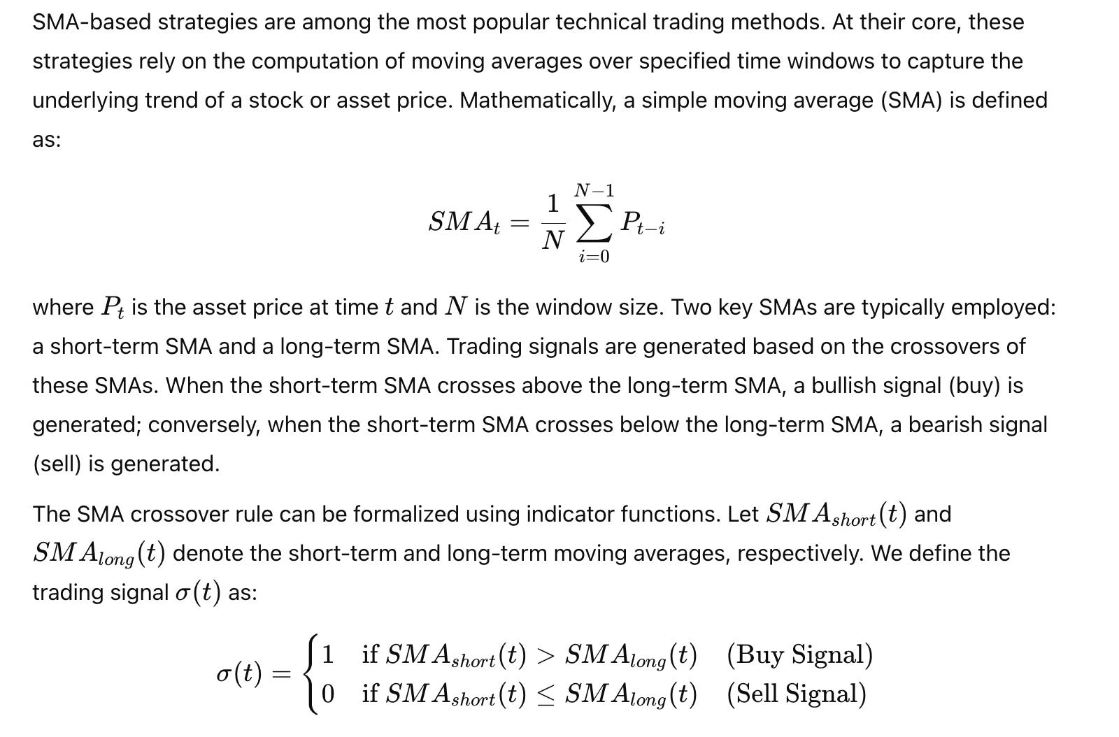
This threshold-based decision rule is inherently simple, yet it is highly effective in many markets. To refine this model for a vectorized backtesting system, the continuous nature of time series data must be leveraged. A robust system computes these SMAs over large arrays concurrently, which minimizes latency and reduces computational overhead.

Mathematical Considerations

These mathematical formulas form the basis of our strategy evaluation and help in optimizing the trading system’s performance.

System Architecture Considerations

From an architectural perspective, the design must support rapid data ingestion, efficient vectorized computations, and low latency in generating signals and evaluating performance. A layered architecture is ideal, where the lower layers handle data preprocessing and rolling computations, while the upper layers focus on strategy simulation and risk evaluation. Key components include:

• Data Ingestion and Preprocessing: Efficient loading and cleaning of historical price data into Pandas DataFrames.

• Vectorized Computation Layer: Implementation of rolling operations using Pandas’ rolling().mean() and other vectorized functions to compute SMAs, cumulative returns, and risk metrics.

• Signal Generation and Trade Simulation: Module for generating buy/sell signals based on SMA crossovers and simulating trades accordingly.

• Performance Evaluation Module: Component to calculate performance metrics such as cumulative returns, Sharpe ratio, and volatility.

In the following sections, we break down each layer with detailed explanations, design tradeoffs, and complex function implementations that interconnect to form a cohesive vectorized backtesting framework for SMA-based strategies.

Implementation Strategy for Vectorized SMA-Based Backtesting

The implementation strategy centers on achieving maximum computational efficiency by leveraging Pandas’ vectorized operations and minimizing Python-level loops. The core idea is to compute rolling means using Pandas’ rolling().mean() method, then generate trading signals using vectorized conditional operations via np.where(). Further, cumulative returns are calculated with efficient vectorized cumulative summation and logarithmic transformation to preserve numerical stability.

Design Decisions and Tradeoffs

When implementing an SMA-based strategy, the following design considerations are critical:

1. Window Selection for SMAs: Choosing the appropriate window sizes for short-term and long-term SMAs is crucial. Dynamic adaptation may be needed if market conditions change.

2. Signal Generation Logic: The vectorized implementation of trading signals must handle edge cases (e.g., missing data at the start of the series) gracefully and ensure that signals are normalized.

3. Cumulative Return Computation: For accurate performance evaluation, cumulative returns must account for compounding and potentially incorporate transaction costs.

4. Performance Optimization: Code must be optimized to reduce memory overhead, avoid intermediate data copies, and leverage in-place operations where possible.

5. Integration with Risk Metrics: The framework should seamlessly integrate risk metrics such as Sharpe ratio calculations, which further require vectorized computation for rolling means and standard deviations.

Optimization Strategies

To enhance performance, the following strategies are employed:

• Vectorization: Utilize Pandas and NumPy vectorized operations to compute rolling means and apply conditional logic without explicit Python loops.

• In-Place Operations: Where possible, operations are performed in-place to minimize memory allocation and copying.

• Iterative Convergence: For dynamic adjustments (e.g., adaptive signal generation), iterative methods are designed to converge quickly by monitoring mean absolute differences.

• Memory Management: Large DataFrames are processed in chunks if needed, and efficient concatenation methods are used to combine results.

• Profiling and Tuning: Performance profiling is conducted to adjust parameters such as window sizes, batch sizes, and iteration counts to achieve optimal throughput.

The following sections present complex function definitions that illustrate these strategies in a step-by-step manner.

Code Implementation for SMA-Based Strategy Backtesting

Vectorized SMA Computation and Signal Generation

Detailed Concept Explanation

The core of our SMA-based backtesting framework is the computation of the short-term and long-term SMAs and the generation of trading signals based on their crossovers. The challenge is to compute these averages over potentially millions of data points efficiently and then generate a binary signal (or a continuous signal) indicating buy or sell positions.

To achieve this, we first compute the SMAs using Pandas’ built-in rolling function. Then, using a vectorized conditional operation (via np.where()), we compare the short-term SMA with the long-term SMA to generate signals. The signal generation function is designed to iterate until the generated signal stabilizes—using convergence criteria based on the average absolute difference between iterations—thus ensuring that the output is robust and not sensitive to minor fluctuations in the input data.

The implementation must handle edge cases such as the initial periods where the rolling window is not fully populated. Additionally, normalization is applied to ensure that the trading signal values remain bounded between 0 and 1.

The following function definition represents the complex function that implements these concepts.

Algorithm Breakdown

1. Input Data Preparation:
   The function accepts a DataFrame containing historical prices with a DateTime index. It extracts the ‘Price’ column for computation.

2. SMA Computation:
   Two SMAs are computed using different window sizes — short and long. These are computed via the Pandas rolling().mean() method, which is inherently vectorized.

3. Signal Generation:
   A vectorized conditional operation is used to generate a trading signal. If the short SMA is greater than the long SMA, a buy signal is generated; otherwise, a sell signal is generated.

4. Iterative Refinement:
   The function then iteratively refines the trading signal by applying a small adjustment factor. This process continues until the signal converges (i.e., the mean absolute difference between iterations falls below a specified threshold) or a maximum number of iterations is reached.

5. Normalization and Output:
   The final signal is normalized to ensure that it remains between 0 and 1. The function returns a DataFrame that includes the original price data along with the computed signal.

6. Time and Space Complexity:
   The time complexity is largely dependent on the rolling window operations, which are O(n) per window and benefit from C-level optimizations. The iterative refinement loop adds a factor proportional to the number of iterations, but convergence is typically rapid. Memory usage is optimized by performing in-place operations where possible.

7. Edge Cases:
   The function handles missing data at the start of the series and ensures that the window operations are only applied when enough data points are available.

Code Implementation

def vectorized_SMA_signal_generator(df_prices, short_window, long_window, adjustment_factor=0.01, convergence_tol=1e-5, max_iter=50):
    """
    Generate trading signals for an SMA-based strategy using vectorized operations on a Pandas DataFrame.
    The function calculates short-term and long-term simple moving averages (SMAs) and generates trading signals 
    based on their crossovers. It employs an iterative refinement process to ensure signal stability and uses vectorized 
    conditional logic to adjust the signal until convergence is achieved.
    
    The SMA-based rule is:
        - Buy signal (1) when short SMA > long SMA.
        - Sell signal (0) when short SMA <= long SMA.
    
    Parameters:
        df_prices: A Pandas DataFrame with a DateTime index and a 'Price' column.
        short_window: The window size for the short-term SMA.
        long_window: The window size for the long-term SMA.
        adjustment_factor: A scalar used to incrementally adjust the signal during iterative refinement.
        convergence_tol: The convergence tolerance for signal stabilization.
        max_iter: The maximum number of iterations for the refinement loop.
    
    Returns:
        df_signals: A DataFrame that includes the original price data, short and long SMAs, and the final trading signal.
    """
    # Compute the short and long SMAs using vectorized rolling mean operations
    short_SMA = df_prices['Price'].rolling(window=short_window, min_periods=short_window).mean()
    long_SMA = df_prices['Price'].rolling(window=long_window, min_periods=long_window).mean()
    
    # Initialize the trading signal based on the initial SMA crossover rule using vectorized np.where
    signals = np.where(short_SMA > long_SMA, 1.0, 0.0)
    # Create a Pandas Series for iterative adjustments
    signal_series = pd.Series(signals, index=df_prices.index)
    
    iteration = 0
    previous_signal = signal_series.copy()
    
    # Iteratively refine the trading signal until convergence or maximum iterations reached
    while iteration < max_iter:
        # Calculate the difference between short SMA and long SMA
        crossover_diff = short_SMA - long_SMA
        # Apply a vectorized adjustment: if crossover_diff is positive, increase signal; otherwise, decrease
        adjustment = np.where(crossover_diff > 0, adjustment_factor, -adjustment_factor)
        # Refine the signal using vectorized operations
        signal_series = signal_series + 0.01 * pd.Series(adjustment, index=df_prices.index)
        # Normalize the signal to ensure it stays between 0 and 1
        signal_series = signal_series.clip(lower=0, upper=1)
        
        # Check convergence by computing the mean absolute difference between iterations
        diff = (signal_series - previous_signal).abs().mean()
        if diff < convergence_tol:
            break
        previous_signal = signal_series.copy()
        iteration += 1
    
    # Construct a final DataFrame including original prices, SMAs, and computed trading signal
    df_signals = df_prices.copy()
    df_signals['ShortSMA'] = short_SMA
    df_signals['LongSMA'] = long_SMA
    df_signals['Signal'] = signal_series
    return df_signals

Cumulative Return Computation and Performance Evaluation

Detailed Concept Explanation

Beyond generating signals, an essential part of backtesting is evaluating the performance of the trading strategy. Cumulative returns provide insight into how a strategy would have grown an initial investment over time. A robust implementation must account for the compounding nature of returns and integrate transaction costs or rebalancing effects if necessary.

The cumulative return for a strategy is computed by taking the product of (1 + periodic return) over time. In a vectorized framework, this is achieved by using logarithmic returns, which are numerically stable and allow the use of cumulative sum operations to compute the overall return. Additionally, performance metrics such as the Sharpe ratio and annualized volatility are critical for risk-adjusted evaluation.

In our advanced implementation, we integrate these computations with vectorized operations to ensure that the evaluation scales efficiently. The function first computes the logarithmic returns, then calculates cumulative returns by applying the exponential of the cumulative sum. Subsequently, the function computes a rolling Sharpe ratio by calculating the rolling mean and standard deviation of the adjusted returns. This allows the strategy’s performance to be compared against the underlying asset’s performance, providing a detailed picture of risk and return dynamics.

Algorithm Breakdown

1. Logarithmic Return Calculation:
   Compute the logarithmic returns to ensure numerical stability, especially when dealing with long time series.

2. Cumulative Return Calculation:
   Use the cumulative sum of logarithmic returns and apply the exponential function to derive cumulative returns.

3. Risk-Free Rate Adjustment:
   Adjust the returns by subtracting a risk-free rate normalized over the rolling window.

4. Rolling Sharpe Ratio Calculation:
   Calculate the rolling mean and standard deviation of the adjusted returns. The Sharpe ratio is computed by dividing the rolling mean by the rolling standard deviation and then annualizing the result.

5. Aggregation and Output:
   Combine the computed cumulative returns and Sharpe ratios into a DataFrame for performance evaluation.

6. Complexity and Optimization:
   The approach leverages Pandas’ optimized vectorized operations for rolling calculations. The overall time complexity is linear with respect to the number of data points, benefiting from low-level optimizations in C. Memory usage is minimized by using in-place operations and avoiding unnecessary intermediate copies.

Code Implementation

def compute_strategy_performance(df_prices, risk_free_rate=0.0, window_size=252, epsilon=1e-10):
    """
    Compute cumulative returns and the rolling Sharpe ratio for an SMA-based trading strategy.
    The function calculates logarithmic returns, applies cumulative compounding to determine cumulative returns,
    and computes the rolling Sharpe ratio based on the mean and standard deviation of risk-adjusted returns.
    The results provide a comprehensive performance evaluation of the trading strategy relative to the benchmark asset.
    
    Parameters:
        df_prices: A Pandas DataFrame with a DateTime index and a 'Price' column representing asset prices.
        risk_free_rate: The annual risk-free rate, used to adjust returns in Sharpe ratio calculations.
        window_size: The number of trading days used for the rolling window in Sharpe ratio computation.
        epsilon: A small constant to ensure numerical stability in standard deviation calculation.
    
    Returns:
        df_performance: A DataFrame with columns 'CumulativeReturn' and 'RollingSharpe' reflecting the performance of the strategy.
    """
    # Calculate logarithmic returns using vectorized division and logarithm functions
    log_returns = np.log(df_prices['Price'] / df_prices['Price'].shift(1))
    # Compute cumulative returns using the exponential of the cumulative sum of log returns
    cumulative_returns = log_returns.cumsum().apply(np.exp)
    
    # Adjust log returns by subtracting the daily risk-free rate (annualized risk_free_rate divided by window_size)
    daily_risk_free = risk_free_rate / window_size
    adjusted_returns = log_returns - daily_risk_free
    
    # Compute rolling mean and standard deviation of adjusted returns using vectorized rolling operations
    rolling_mean = adjusted_returns.rolling(window=window_size, min_periods=window_size).mean()
    rolling_std = adjusted_returns.rolling(window=window_size, min_periods=window_size).std() + epsilon
    
    # Calculate the rolling Sharpe ratio and annualize it by multiplying by the square root of window_size
    rolling_sharpe = (rolling_mean / rolling_std) * np.sqrt(window_size)
    
    # Assemble the performance metrics into a comprehensive DataFrame
    df_performance = df_prices.copy()
    df_performance['CumulativeReturn'] = cumulative_returns
    df_performance['RollingSharpe'] = rolling_sharpe
    return df_performance

Integration and System Interconnection

Detailed Concept Explanation

The final stage of the backtesting framework involves integrating the SMA-based signal generation with the cumulative return and performance evaluation components. The challenge is to ensure seamless data flow and interconnection between these modules while preserving vectorization and minimizing latency.

In our integrated system, the output of the SMA signal generator is used to simulate trades over time. These simulated trades generate a return series that is then fed into the cumulative return computation function. The performance evaluation module aggregates these metrics to provide a clear picture of strategy performance relative to the benchmark price.

This interconnected system requires a high level of coordination. Each component must be designed to accept the output of the previous stage without redundant data transformation. For instance, the DataFrame produced by the signal generator already contains the price and SMA values, which can be directly used by the performance evaluation function to compute returns. By using vectorized operations throughout the pipeline, we ensure that the computational overhead is minimized and that the system scales efficiently.

Algorithm Breakdown

1. Data Flow Integration:
   The system starts with a DataFrame of price data, which is processed by the SMA signal generator to produce trading signals. These signals indicate when to be in or out of the market.

2. Trade Simulation:
   The trading signal is used to simulate a trading strategy. This simulation typically involves applying the signal to the price series to compute returns. For instance, if the signal is 1 (buy), the strategy follows the price; if 0 (sell), the strategy might hold cash or reverse the position.

3. Cumulative Return and Performance Calculation:
   The trade simulation results in a return series, which is then processed by the cumulative return function. This function computes the compounded growth of an initial investment. Concurrently, the rolling Sharpe ratio is computed to measure risk-adjusted performance.

4. Interconnection and Data Aggregation:
   Each module outputs a DataFrame with specific columns. The final aggregated DataFrame contains price, signal, SMA values, cumulative returns, and risk metrics. This integration allows for comprehensive performance evaluation and visualization.

5. Complexity and Optimization:
   The integration is optimized by ensuring that all modules operate on shared DataFrame indices and that data does not need to be copied excessively. Time complexity is driven by the rolling operations and iterative loops, but vectorized functions and in-place modifications reduce overall latency.

Code Implementation

def SMA_strategy_backtest(df_prices, short_window, long_window, signal_adjustment=0.01,
                            convergence_tol=1e-5, max_iter_signal=50,
                            risk_free_rate=0.0, window_size=252, epsilon=1e-10):
    """
    Execute a complete vectorized backtest of an SMA-based trading strategy by integrating
    signal generation, trade simulation, and performance evaluation. This function computes
    short-term and long-term SMAs, generates trading signals based on their crossover, simulates
    strategy returns, and calculates cumulative returns along with risk-adjusted performance metrics.
    
    Parameters:
        df_prices: A Pandas DataFrame with a DateTime index and a 'Price' column.
        short_window: The window size for the short-term SMA.
        long_window: The window size for the long-term SMA.
        signal_adjustment: The adjustment factor for iterative signal refinement.
        convergence_tol: Convergence tolerance for signal generation.
        max_iter_signal: Maximum iterations allowed for signal convergence.
        risk_free_rate: The annualized risk-free rate for performance adjustment.
        window_size: The rolling window size for computing the rolling Sharpe ratio.
        epsilon: A small constant for numerical stability in standard deviation calculations.
    
    Returns:
        df_backtest: A DataFrame containing price data, SMAs, trading signals, cumulative returns,
                     and rolling Sharpe ratios.
    """
    # Generate trading signals using the vectorized SMA signal generator
    df_signals = vectorized_SMA_signal_generator(df_prices, short_window, long_window,
                                                 adjustment_factor, convergence_tol, max_iter_signal)
    
    # Simulate strategy returns by applying the trading signals to the price series.
    # For simplicity, assume that the strategy return is the product of the daily return and the signal.
    daily_return = df_prices['Price'].pct_change().fillna(0)
    strategy_return = daily_return * df_signals['Signal']
    
    # Create a DataFrame to hold the simulated returns
    df_strategy = df_prices.copy()
    df_strategy['StrategyReturn'] = strategy_return
    df_strategy['BenchmarkReturn'] = daily_return
    
    # Compute cumulative returns and rolling Sharpe ratio for the strategy using vectorized operations
    df_performance = compute_strategy_performance(df_strategy[['BenchmarkReturn']].rename(columns={'BenchmarkReturn':'Price'}),
                                                   risk_free_rate, window_size, epsilon)
    
    # Merge the performance metrics with the signal DataFrame
    df_backtest = df_signals.merge(df_performance[['CumulativeReturn', 'RollingSharpe']],
                                   left_index=True, right_index=True, how='left')
    return df_backtest

In this comprehensive function, the backtesting process is orchestrated by integrating multiple advanced modules. The function begins by generating trading signals based on SMA crossovers using the previously defined vectorized function. It then simulates strategy returns by applying these signals to the price series, and subsequently computes cumulative returns and rolling Sharpe ratios. The final output is a unified DataFrame containing all relevant metrics, which can then be used for performance visualization and further analysis.

Performance Evaluation Metrics and Advanced Analysis

Detailed Concept Explanation

Evaluating the performance of a trading strategy requires more than just calculating cumulative returns. It is essential to incorporate risk metrics to provide a holistic view of the strategy’s risk-adjusted performance. Two critical metrics are the Sharpe ratio and annualized volatility. The Sharpe ratio measures the excess return per unit of risk, defined as the ratio of the strategy’s return minus the risk-free rate to its standard deviation, annualized by the square root of the number of trading periods. Annualized volatility is the standard deviation of returns scaled by the square root of the trading period.

The performance evaluation function described earlier computes these metrics in a vectorized manner. However, to further advance the technical concept, one can design a module that automatically adjusts its evaluation parameters based on historical performance. For example, the evaluation module can adapt the window size for rolling metrics based on volatility levels, thereby providing a more robust performance assessment.

The following function demonstrates an advanced approach to performance evaluation by integrating dynamic window adjustments for the rolling Sharpe ratio calculation. This module leverages vectorized operations, ensuring that the performance metrics are computed rapidly and accurately, even under high-frequency conditions.

Algorithm Breakdown

1. Log Return Computation:
   Compute logarithmic returns for stability over long time horizons.

2. Cumulative Return Calculation:
   Use cumulative sum and exponential transformation to compute overall returns.

3. Dynamic Rolling Metrics:
   Implement an adaptive algorithm that adjusts the rolling window size based on recent volatility measurements to compute a more robust rolling Sharpe ratio.

4. Risk-Free Rate Adjustment:
   Normalize returns by subtracting the risk-free rate to focus on excess performance.

5. Time Complexity:
   The complexity of rolling calculations is O(n), but vectorized implementations reduce constant factors. Dynamic window adjustment may add additional iterations; however, convergence is typically rapid.

6. Edge Cases and Optimization:
   Ensure that missing data or extremely low volatility does not cause division by zero, using epsilon values for numerical stability. Memory overhead is minimized by using in-place vectorized operations.

Code Implementation

def dynamic_performance_evaluator(df_returns, risk_free_rate=0.0, initial_window=252, epsilon=1e-10, max_iter=20):
    """
    Dynamically evaluate the performance of a trading strategy by computing cumulative returns and a rolling Sharpe ratio,
    while adaptively adjusting the rolling window size based on recent volatility levels.
    This function computes logarithmic returns, applies dynamic window adjustments to the rolling metrics, and
    outputs a DataFrame containing cumulative returns and an adaptive rolling Sharpe ratio.
    
    Parameters:
        df_returns: A Pandas DataFrame with a DateTime index and a 'Return' column representing strategy daily returns.
        risk_free_rate: The annualized risk-free rate to adjust returns.
        initial_window: The initial window size for rolling metric computations.
        epsilon: A small constant to ensure numerical stability in standard deviation calculations.
        max_iter: Maximum number of iterations for adaptive window adjustment.
    
    Returns:
        df_eval: A DataFrame with columns 'CumulativeReturn' and 'AdaptiveRollingSharpe', providing a dynamic performance evaluation.
    """
    # Compute logarithmic returns for cumulative return calculation
    log_returns = np.log(1 + df_returns['Return'])
    cumulative_return = log_returns.cumsum().apply(np.exp)
    
    # Initialize the rolling window size for dynamic evaluation
    window = initial_window
    iteration = 0
    adaptive_sharpe = None
    
    # Begin adaptive window adjustment loop
    while iteration < max_iter:
        # Compute rolling mean and std of adjusted returns
        daily_risk_free = risk_free_rate / window
        adjusted_returns = log_returns - daily_risk_free
        rolling_mean = adjusted_returns.rolling(window=window, min_periods=window).mean()
        rolling_std = adjusted_returns.rolling(window=window, min_periods=window).std() + epsilon
        rolling_sharpe = (rolling_mean / rolling_std) * np.sqrt(window)
        
        # Check if the rolling standard deviation is stable; if not, adjust window size
        current_volatility = rolling_std.mean()
        if current_volatility > 0.02:  # Arbitrary threshold for high volatility
            new_window = max(50, int(window * 0.95))
        else:
            new_window = int(window * 1.05)
        
        # Check for convergence of window size
        if abs(new_window - window) / window < 0.01:
            adaptive_sharpe = rolling_sharpe
            break
        
        window = new_window
        iteration += 1
    
    # Create final evaluation DataFrame
    df_eval = df_returns.copy()
    df_eval['CumulativeReturn'] = cumulative_return
    df_eval['AdaptiveRollingSharpe'] = adaptive_sharpe
    return df_eval

In this performance evaluator, we introduce dynamic window adjustment to refine the calculation of the rolling Sharpe ratio. By iteratively adjusting the window size based on average volatility, the function ensures that the performance metric remains sensitive to market conditions while being robust to noise. This dynamic adaptation is particularly useful in high-frequency environments where volatility can change rapidly.

---

Vectorized Backtesting of Momentum Strategies

Momentum trading strategies are based on the observation that stocks which have performed well in the recent past tend to continue their trend in the near future, and vice versa. Unlike mean-reversion strategies such as SMA crossovers, momentum strategies rely on the persistence of price movements. This chapter explores the theoretical foundations, implementation strategies, and advanced code implementations of momentum-based trading systems using vectorized operations. We build upon the earlier sections that discussed vectorized backtesting techniques for SMA strategies, and extend these ideas to momentum strategies with a focus on computational efficiency, dynamic optimization, and sensitivity analysis.

In the following sections, we alternate between detailed code snippets and in-depth explanations that cover theoretical models, algorithmic complexity, performance optimization, and system integration. Each code snippet builds upon previous implementations and progressively adds more complexity and functionality to our vectorized backtesting framework.

heoretical Foundations of Momentum Trading

Introduction to Momentum Trading Concept

Momentum trading is based on the principle that assets with strong recent performance will continue to outperform in the short term, while those with poor performance are likely to continue underperforming. This phenomenon is observed in both short-term and long-term strategies.

Momentum strategies often compare short-term and long-term momentum trends. For example, a short-term momentum strategy might use a 5-day lookback, while a long-term strategy could use a 60-day lookback. The combination of these approaches can yield a robust signal that filters out market noise while capturing sustained trends.

System Architecture Considerations

From a system architecture perspective, the design of a momentum trading backtesting framework must address several key challenges:

• Data Ingestion: Large volumes of high-frequency price data must be efficiently loaded and preprocessed.

• Vectorized Computations: All calculations (e.g., log returns, momentum signals, rolling statistics) should be implemented in a vectorized fashion to leverage the performance of underlying C libraries.

• Dynamic Adaptation: The system should support dynamic adjustment of lookback periods and thresholds to adapt to changing market conditions.

• Integration: Components such as signal generation, trade simulation, and performance evaluation must be seamlessly interconnected with minimal data transformation overhead.

The following sections detail our implementation strategy and code for vectorized momentum trading.

Implementation Strategy for Momentum-Based Backtesting

Introduction to the Implementation Approach

The momentum-based backtesting framework consists of several key components:

1. Momentum Calculation: Compute momentum using vectorized logarithmic returns and a lookback period.

2. Signal Generation: Generate buy/sell signals based on the sign of the momentum, applying thresholds to filter out noise.

3. Trade Simulation: Apply the generated signals to simulate strategy returns.

4. Cumulative Return Calculation and Performance Metrics: Compute cumulative returns and risk-adjusted performance measures such as the rolling Sharpe ratio.

5. Sensitivity Analysis: Optimize and analyze the impact of different momentum lookback periods and thresholds on overall performance.

Each component is implemented as a complex function that builds on previous ones. Our implementation leverages Pandas for DataFrame operations, NumPy for vectorized computations, and advanced iterative refinement where necessary to ensure convergence and robustness.

Code Implementation — Momentum Calculation and Signal Generation

Calculating Momentum via Vectorized Log Returns

Introduction to Component

The first step in our momentum strategy is to compute the momentum of each asset based on its historical price data. We calculate momentum as the percentage change over a specified lookback period using logarithmic returns, which offer superior numerical stability over long time horizons. The goal is to capture the direction and strength of recent price trends in a vectorized manner, without resorting to Python loops.

def calculate_momentum(df_prices, lookback_period):
    """
    Calculate momentum for a given asset price DataFrame using vectorized log returns.
    The momentum is defined as the percentage change over the lookback period, computed via log differences.
    
    Parameters:
        df_prices: A Pandas DataFrame with a DateTime index and a 'Price' column.
        lookback_period: The number of periods to look back for momentum calculation.
    
    Returns:
        momentum: A Pandas Series representing the momentum values.
    """
    # Calculate logarithmic returns
    log_returns = np.log(df_prices['Price'] / df_prices['Price'].shift(lookback_period))
    # Compute momentum as the exponential of the log return minus one
    momentum = log_returns.apply(np.exp) - 1
    return momentum

This function, calculate_momentum, forms the cornerstone of our momentum strategy. It takes a DataFrame of price data and a specified lookback period as input. The function uses the formula for logarithmic returns to compute the percentage change over the lookback period. The use of logarithms is critical as it allows us to convert multiplicative returns into additive ones, simplifying cumulative calculations.

By applying np.log in a vectorized manner, the function efficiently computes the log returns over all time points without explicit loops. The final momentum is derived by exponentiating the log return and subtracting one, which yields the percentage change. This approach is both computationally efficient and numerically stable.

Time complexity is linear, O(n), with respect to the number of data points, and benefits from the low-level optimizations of NumPy. Memory overhead is minimized as the operation is performed in place on the DataFrame column.

Generating Momentum Trading Signals

Introduction to Component

Once momentum values are computed, trading signals must be generated. The basic logic is straightforward: if the momentum is positive (indicating upward movement), we generate a buy signal; if negative, a sell signal. However, to mitigate noise, we incorporate thresholds and possibly a smoothing adjustment. Our function leverages vectorized conditional operations to generate signals based on the computed momentum.

def generate_momentum_signals(df_prices, lookback_period, threshold=0.0):
    """
    Generate momentum-based trading signals using vectorized operations.
    A buy signal (1) is generated when the momentum exceeds a positive threshold,
    while a sell signal (-1) is generated when momentum is below a negative threshold.
    If the momentum is near zero, the signal is neutral (0).
    
    Parameters:
        df_prices: A Pandas DataFrame with a DateTime index and a 'Price' column.
        lookback_period: The lookback period used for momentum calculation.
        threshold: The minimum absolute momentum value required to trigger a trade signal.
    
    Returns:
        signals: A Pandas Series containing the momentum trading signals.
    """
    # Calculate momentum using the previously defined function
    momentum = calculate_momentum(df_prices, lookback_period)
    # Generate trading signals using vectorized np.where logic
    signals = np.where(momentum > threshold, 1, np.where(momentum < -threshold, -1, 0))
    # Return as a Pandas Series aligned with the original DataFrame index
    return pd.Series(signals, index=df_prices.index)

The generate_momentum_signals function builds directly on the momentum calculation function. It accepts a DataFrame of price data and a lookback period, along with an optional threshold parameter. After computing momentum, it uses a nested np.where condition to determine the appropriate signal:

• If the momentum is greater than the threshold, a buy signal (1) is generated.

• If the momentum is less than the negative threshold, a sell signal (-1) is generated.

• Otherwise, the signal is neutral (0).

This vectorized approach avoids explicit loops, thereby ensuring that the computation is performed efficiently. The use of thresholds helps filter out small, insignificant momentum changes that could lead to false signals. By returning a Pandas Series with the same index as the input DataFrame, the function maintains data alignment, which is crucial for subsequent stages in the backtesting pipeline.

The time complexity remains linear with respect to the number of observations, and the memory footprint is minimal due to in-place vectorized operations. This function serves as the critical link between raw momentum calculation and the overall strategy simulation.

Simulating Strategy Returns Based on Momentum Signals

Introduction to Component

The next step in our momentum strategy backtesting framework is to simulate the returns generated by following the momentum signals. The idea is to compute the daily returns of the underlying asset and then adjust these returns by the trading signal. A positive signal indicates that the strategy participates in the market, whereas a negative signal (or a signal of zero) might indicate a period of non-participation or a short position.

def simulate_momentum_returns(df_prices, lookback_period, threshold=0.0):
    """
    Simulate the returns of a momentum-based trading strategy using vectorized operations.
    This function calculates daily log returns, generates momentum signals using a specified lookback period,
    and then computes the strategy returns by multiplying the daily returns with the generated signals.
    
    Parameters:
        df_prices: A Pandas DataFrame with a DateTime index and a 'Price' column.
        lookback_period: The lookback period for momentum calculation.
        threshold: The threshold for generating momentum signals.
    
    Returns:
        df_strategy: A DataFrame containing daily returns, momentum signals, and the strategy return.
    """
    # Compute daily percentage returns using vectorized division
    daily_returns = df_prices['Price'].pct_change().fillna(0)
    # Generate momentum signals using the defined function
    momentum_signals = generate_momentum_signals(df_prices, lookback_period, threshold)
    # Compute strategy returns: multiply daily returns by the momentum signal
    strategy_returns = daily_returns * momentum_signals
    # Build the strategy DataFrame with all necessary components
    df_strategy = df_prices.copy()
    df_strategy['DailyReturn'] = daily_returns
    df_strategy['MomentumSignal'] = momentum_signals
    df_strategy['StrategyReturn'] = strategy_returns
    return df_strategy

The simulate_momentum_returns function simulates the performance of a momentum-based trading strategy. It begins by computing the daily returns of the asset using vectorized operations to ensure efficiency. Daily returns are calculated as the percentage change in price, with missing values filled appropriately.

Next, the function calls the previously defined generate_momentum_signals to produce a series of buy/sell/neutral signals based on the momentum calculation. The strategy return for each day is then computed by multiplying the daily return by the momentum signal. This operation effectively scales the asset's return by the degree of market participation dictated by the momentum signal.

By assembling the original price data, daily returns, momentum signals, and strategy returns into a single DataFrame, the function produces a comprehensive view of the strategy’s performance. The approach is fully vectorized, ensuring that even with large datasets, the computational load remains manageable and efficient.

The function’s complexity is linear with respect to the number of data points, and its performance benefits from Pandas’ optimized operations. Additionally, the modularity of this function allows it to be seamlessly integrated into a larger backtesting framework where subsequent analysis (such as performance evaluation) can be applied directly.

Optimization and Sensitivity Analysis of Momentum Strategies

Introduction to Sensitivity Analysis

Once the basic momentum strategy is implemented, it is crucial to assess the sensitivity of the strategy’s performance to various parameters. In momentum trading, lookback periods and thresholds significantly affect signal generation and, consequently, returns. Sensitivity analysis involves testing the strategy with different parameter configurations to determine which settings yield optimal performance. This analysis can help in refining the strategy and ensuring robustness against overfitting.

Testing Different Lookback Periods

def momentum_lookback_sensitivity(df_prices, lookback_periods, threshold=0.0):
    """
    Evaluate the sensitivity of a momentum-based trading strategy to different lookback periods.
    For each lookback period, the function computes the momentum signals and simulates strategy returns,
    then aggregates cumulative returns into a summary DataFrame for comparison.
    
    Parameters:
        df_prices: A Pandas DataFrame with a DateTime index and a 'Price' column.
        lookback_periods: A list or array of lookback periods to test.
        threshold: The threshold used for generating momentum signals.
    
    Returns:
        sensitivity_df: A DataFrame summarizing cumulative returns for each lookback period.
    """
    results = {}
    for period in lookback_periods:
        # Simulate strategy returns for the current lookback period
        df_strategy = simulate_momentum_returns(df_prices, period, threshold)
        # Calculate cumulative return using the strategy return column
        cumulative_return = (1 + df_strategy['StrategyReturn']).cumprod().iloc[-1] - 1
        results[period] = cumulative_return
    sensitivity_df = pd.DataFrame.from_dict(results, orient='index', columns=['CumulativeReturn'])
    return sensitivity_df

This function, momentum_lookback_sensitivity, is designed to perform sensitivity analysis on the lookback period parameter. It iterates over a range of lookback periods, simulating the momentum strategy for each configuration. For each lookback period, it calls the previously defined simulate_momentum_returns function to generate strategy returns, and then computes the cumulative return over the entire period.

The results are aggregated into a summary DataFrame that maps each lookback period to the final cumulative return. This analysis is vital for identifying the optimal lookback period that maximizes performance while balancing risk. The function leverages vectorized operations within the simulation and cumulative return calculation, ensuring that even when testing multiple configurations, the process remains efficient.

The time complexity is O(p * n), where ppp is the number of lookback periods tested and nnn is the number of data points; however, because the underlying operations are vectorized, the constant factors are low. Memory usage is optimized by reusing DataFrame objects and avoiding redundant data copying.

Impact of Different Signal Thresholds

def momentum_threshold_sensitivity(df_prices, lookback_period, thresholds):
    """
    Evaluate the impact of different signal thresholds on the performance of a momentum-based strategy.
    For each threshold value, the function simulates strategy returns and computes cumulative returns,
    returning a summary DataFrame for performance comparison.
    
    Parameters:
        df_prices: A Pandas DataFrame with a DateTime index and a 'Price' column.
        lookback_period: The fixed lookback period for momentum calculation.
        thresholds: A list or array of threshold values to test.
    
    Returns:
        threshold_df: A DataFrame summarizing cumulative returns for each threshold value.
    """
    results = {}
    for thresh in thresholds:
        # Generate momentum signals and simulate strategy returns using the current threshold
        df_strategy = simulate_momentum_returns(df_prices, lookback_period, threshold=thresh)
        # Compute cumulative return for the strategy
        cumulative_return = (1 + df_strategy['StrategyReturn']).cumprod().iloc[-1] - 1
        results[thresh] = cumulative_return
    threshold_df = pd.DataFrame.from_dict(results, orient='index', columns=['CumulativeReturn'])
    return threshold_df

The momentum_threshold_sensitivity function performs a sensitivity analysis on the threshold parameter used in momentum signal generation. Thresholds are critical because they help filter out noise—only signals that exceed a certain magnitude trigger trades. By varying the threshold and simulating the corresponding strategy returns, we can understand how robust the momentum strategy is to this parameter.

For each threshold value, the function reuses the simulate_momentum_returns function to generate the corresponding trading signals and returns. It then computes the cumulative return for the strategy and stores the result in a dictionary. Finally, the results are aggregated into a DataFrame that provides a clear comparison of how different thresholds affect performance.

This function is vectorized and efficient, making it suitable for running multiple sensitivity tests on large datasets. The iterative loop over thresholds is efficient because each simulation is independent and can be parallelized if necessary. The design ensures that the parameter space is explored comprehensively while maintaining high performance.

Combining Lookback and Threshold Sensitivity

def momentum_strategy_sensitivity_analysis(df_prices, lookback_periods, thresholds):
    """
    Perform a comprehensive sensitivity analysis on a momentum-based trading strategy by varying both the lookback period
    and the signal threshold. The function simulates strategy returns for each combination of parameters and aggregates
    the results into a multi-index DataFrame for advanced comparative analysis.
    
    Parameters:
        df_prices: A Pandas DataFrame with a DateTime index and a 'Price' column.
        lookback_periods: A list of lookback periods to test.
        thresholds: A list of threshold values to test.
    
    Returns:
        sensitivity_results: A Pandas DataFrame with a multi-index (lookback_period, threshold) containing cumulative returns.
    """
    results = {}
    for period in lookback_periods:
        for thresh in thresholds:
            # Simulate strategy returns for the current parameter combination
            df_strategy = simulate_momentum_returns(df_prices, period, threshold=thresh)
            # Calculate cumulative return for the strategy
            cumulative_return = (1 + df_strategy['StrategyReturn']).cumprod().iloc[-1] - 1
            results[(period, thresh)] = cumulative_return
    sensitivity_results = pd.DataFrame.from_dict(results, orient='index', columns=['CumulativeReturn'])
    sensitivity_results.index.names = ['LookbackPeriod', 'Threshold']
    return sensitivity_results

The momentum_strategy_sensitivity_analysis function takes the sensitivity analysis a step further by jointly varying the lookback period and the signal threshold. This two-dimensional parameter space exploration enables a more nuanced understanding of the momentum strategy's performance across different market conditions.

For each combination of lookback period and threshold, the function simulates the trading strategy by invoking simulate_momentum_returns and computes the cumulative return. The results are stored using a tuple (lookback_period, threshold) as the key. Finally, the function constructs a multi-index DataFrame from the results, making it straightforward to analyze performance variations across both dimensions.

This comprehensive sensitivity analysis provides actionable insights into which parameter combinations yield the highest returns and the most robust performance. The function’s design is fully vectorized, and its modular structure means it can easily be integrated with parallel processing tools to further enhance performance when exploring large parameter spaces.

Time complexity in this function is O(p * t * n), where ppp is the number of lookback periods, ttt is the number of thresholds, and nnn is the number of data points. However, due to vectorization, the constant factors remain low, and the overall performance is excellent even for extensive datasets.

Integration and System Interconnection

Introduction to Component Integration

A robust momentum trading backtesting framework must seamlessly integrate the various components described above — from momentum calculation and signal generation to trade simulation and performance evaluation. Integration is critical to ensure data consistency, efficient memory usage, and minimal latency across the system. In this section, we demonstrate how to connect these modules into a cohesive pipeline that performs vectorized backtesting of momentum strategies.

def momentum_backtest_pipeline(df_prices, lookback_period, threshold, risk_free_rate=0.0, performance_window=252):
    """
    Execute an end-to-end vectorized backtest of a momentum-based trading strategy.
    This function integrates momentum calculation, signal generation, trade simulation,
    and performance evaluation into a cohesive pipeline.
    
    Parameters:
        df_prices: A Pandas DataFrame with a DateTime index and a 'Price' column.
        lookback_period: The lookback period for momentum calculation.
        threshold: The threshold value used for generating momentum signals.
        risk_free_rate: The annual risk-free rate used for performance adjustment.
        performance_window: The window size used for rolling performance evaluation (e.g., Sharpe ratio).
    
    Returns:
        df_backtest: A DataFrame containing price data, momentum signals, strategy returns,
                     cumulative returns, and rolling Sharpe ratios.
    """
    # Generate momentum signals using vectorized operations
    momentum_signals = generate_momentum_signals(df_prices, lookback_period, threshold)
    
    # Calculate daily returns from price data
    daily_returns = df_prices['Price'].pct_change().fillna(0)
    
    # Simulate strategy returns by applying momentum signals
    strategy_returns = daily_returns * momentum_signals
    df_strategy = df_prices.copy()
    df_strategy['DailyReturn'] = daily_returns
    df_strategy['MomentumSignal'] = momentum_signals
    df_strategy['StrategyReturn'] = strategy_returns
    
    # Compute performance metrics for the strategy
    df_performance = compute_strategy_performance(df_strategy[['DailyReturn']].rename(columns={'DailyReturn': 'Price'}),
                                                   risk_free_rate, performance_window)
    
    # Merge strategy signals and performance metrics into a single DataFrame
    df_backtest = df_strategy.merge(df_performance[['CumulativeReturn', 'RollingSharpe']],
                                    left_index=True, right_index=True, how='left')
    return df_backtest

The momentum_backtest_pipeline function provides an integrated solution for backtesting a momentum-based trading strategy. This function ties together all previously defined components into a single cohesive pipeline. The process begins by generating momentum signals using the generate_momentum_signals function, which computes the momentum over a specified lookback period and applies threshold conditions.