

Momentum-Based Long–Short Trading Strategy
Building, backtesting, and statistically validating a portfolio that buys top-performing stocks and shorts underperformers using historical return momentum.

Download source code using the button at the end of this article
Packages
We also import helper, project_helper, and project_tests. These custom packages support problem-solving. The helper and project_helper modules provide utility and graphing functions, while project_tests includes the unit tests.
Install Packages
import subprocess
command_line = f”{sys.executable} -m pip install -r requirements.txt”
subprocess.run(command_line, shell=True)
This code snippet serves as an initialization step in our momentum trading system, ensuring that the Python environment is equipped with all required dependencies before the core trading logic — such as signal generation, backtesting, and execution strategies — can proceed reliably. It begins by constructing a shell command string that leverages the current Python interpreter to invoke pip, the package installer, specifically targeting the requirements.txt file which lists all necessary libraries like those for data analysis, financial modeling, and algorithmic trading. By using sys.executable in the f-string, the command dynamically references the exact path to the Python executable in use at runtime, guaranteeing compatibility and preventing issues from mismatched interpreter versions that could disrupt momentum calculations or market data processing. The subprocess module’s run function then executes this command with shell=True, allowing the operating system shell to interpret and run it as a native process; this approach is chosen to handle the pip installation seamlessly within the script’s context, installing packages directly into the active environment so that subsequent modules for momentum indicator computations, such as rate-of-change metrics or moving average crossovers, have immediate access to tools like NumPy, pandas, or specialized finance libraries without manual intervention.
Loading Packages
import pandas as pd
import numpy as np
import helper
import project_helper
import project_tests
The provided code block initializes the necessary dependencies for a momentum trading analysis pipeline by importing key libraries and modules. Pandas is brought in as ‘pd’ to facilitate efficient manipulation of financial time-series data, such as stock prices and volumes, which are central to identifying momentum signals like upward trends in asset performance. NumPy, aliased as ‘np’, supports vectorized numerical operations essential for computing momentum indicators, such as rate-of-change calculations or rolling averages, ensuring scalable processing of large datasets without performance bottlenecks. The ‘helper’ and ‘project_helper’ modules import custom utility functions tailored to the project, likely encapsulating reusable logic for data preprocessing, feature engineering, or signal generation specific to momentum strategies, where the goal is to capitalize on persistent price trends. Finally, ‘project_tests’ imports testing utilities to validate the implementation against expected momentum trading behaviors, such as backtesting signal accuracy on historical data to confirm profitable entry and exit points. This setup ensures the environment is primed for sequential data flow — from loading market data, to applying momentum computations, to evaluating trading outcomes — directly supporting the objective of developing robust momentum-based trading models.
Market Data
Loading Data
The data used in most projects consists of end-of-day market data. This dataset includes information for numerous stocks, though the analysis focuses on those in the S&P 500. To facilitate efficient processing, the time period has been narrowed rather than using the full dataset.
df = pd.read_csv(’../../data/project_1/eod-quotemedia.csv’, index_col=False)
df[’date’] = pd.to_datetime(df[’date’])
close = df.set_index([’date’, ‘ticker’])[’adj_close’].unstack(fill_value=None)
print(’Loaded Data’)
The code begins by loading historical end-of-day stock data from a CSV file into a pandas DataFrame, which serves as the foundational dataset for momentum trading analysis. In momentum trading strategies, we rely on time-series price data across multiple tickers to identify trends and calculate metrics like relative strength or rate-of-change, so this step ingests the raw data — likely containing columns such as date, ticker symbols, and adjusted closing prices — from a structured file located at a relative path, ensuring all rows and columns are preserved without setting any index initially to maintain flexibility in data manipulation.
Next, the ‘date’ column is converted to a pandas datetime format, which is essential for chronological ordering and time-based operations in momentum trading. This transformation enables accurate sorting, filtering by periods (e.g., daily, weekly), and computations of returns over specific horizons, such as 12-month momentum, by treating dates as proper temporal objects rather than strings, thus preventing errors in subsequent slicing or aggregation.
The data is then restructured by setting a multi-index on ‘date’ and ‘ticker’, selecting only the ‘adj_close’ column (adjusted closing prices, which account for dividends and splits to provide a clean basis for performance measurement), and unstacking it with None as the fill value for missing entries. This pivots the DataFrame into a wide format where rows represent unique dates, columns represent tickers, and cell values are the corresponding adjusted closing prices, filling any gaps with None to avoid artificial interpolation that could distort momentum signals. For momentum trading, this organization facilitates efficient matrix operations, such as computing percentage changes across tickers for each date or ranking assets by trailing returns, streamlining the identification of high-momentum opportunities without nested loops or repeated grouping.
Finally, a simple print statement confirms the data loading process has completed successfully, providing a checkpoint in the workflow to verify that the dataset is ready for downstream momentum calculations.
View Data
Run the cell below to examine the data for close.
close.iloc[:5]Iwhere strategies rely on analyzing historical price trends to identify assets gaining upward velocity, the code close.iloc[:5] accesses the first five rows of the close pandas Series or DataFrame, which typically stores closing prices from financial market data. This integer-location (iloc) indexing operation slices the data starting from the beginning (index 0) up to but not including the fifth position, effectively retrieving an initial subset of the time series for examination. By focusing on these early observations, the code enables a preliminary view of the price sequence, which is foundational for subsequent momentum calculations, such as computing short-term returns or momentum indicators that assess whether prices are accelerating to signal potential buy opportunities. The selection preserves the original data types and structure, ensuring that the extracted values can be directly used in downstream vectorized operations without altering the broader dataset.
Stock Example
This example examines the closing prices for a single stock. For this and all subsequent display examples in this project, we use Apple’s stock (AAPL). Graphing all stocks would present an overwhelming amount of information.
project_helper.plot_stock(close[’AAPL’], ‘AAPL Stock’)This line of code invokes the plot_stock function from the project_helper module to generate a visualization of the closing prices for Apple Inc. (AAPL) stock, serving as a foundational step in momentum trading analysis by providing a clear graphical representation of historical price movements. The process begins with accessing the ‘AAPL’ key or column from the close data structure, which contains the time-series closing price data for various stocks; this extraction isolates the relevant AAPL price sequence, ensuring that only the pertinent data is passed forward for rendering. The function then receives this AAPL price data as its first argument and the string ‘AAPL Stock’ as the second, which acts as the plot’s title to contextualize the visualization specifically for AAPL. By plotting these closing prices, the code facilitates the identification of upward or downward momentum trends over time — key to momentum trading strategies that rely on detecting sustained price directions to inform buy or sell decisions — without altering the underlying data, simply transforming it into a line chart or similar format for immediate interpretive insight.
Resample Adjusted Prices
The trading signal you develop in this project is not limited to daily prices. For example, you can use month-end prices to execute trades once a month. To do this, first resample the daily adjusted closing prices into monthly intervals, selecting the last observation for each month.
Implement the resample_prices function to resample close_prices at the specified sampling frequency freq.
def resample_prices(close_prices, freq=’M’):
    “”“
    Resample close prices for each ticker at specified frequency.

    Parameters
    ----------
    close_prices : DataFrame
        Close prices for each ticker and date
    freq : str
        What frequency to sample at
        For valid freq choices, see http://pandas.pydata.org/pandas-docs/stable/timeseries.html#offset-aliases

    Returns
    -------
    prices_resampled : DataFrame
        Resampled prices for each ticker and date
    “”“
    # TODO: Implement Function
    # <DataFrame or Series>.resample(arguments).<aggregate function>
    import pandas as pd
    aggregated_data = close_prices.groupby(pd.Grouper(freq=freq)).last()

    return aggregated_data
The resample_prices function processes a DataFrame of close prices, indexed by dates for multiple tickers, to aggregate them at a specified frequency, such as monthly (‘M’), which is essential in momentum trading strategies where we rely on end-of-period prices to calculate returns and momentum signals without the influence of daily fluctuations. It begins by importing the pandas library, ensuring the necessary tools for time-series manipulation are available within the function’s scope. The core logic then applies a groupby operation using pd.Grouper(freq=freq), which organizes the data into time-based groups aligned to the target frequency — for instance, grouping all daily closes within each month into a single unit. This grouping respects the DataFrame’s date index, allowing pandas to automatically handle irregular date ranges and align boundaries, such as starting months on the first day. To aggregate within each group, the function calls .last() on the grouped data, selecting the final close price in every period as the representative value; this choice ensures we capture the most recent market close for that frequency, which is critical for momentum calculations that depend on accurate period-end snapshots to measure price trends over time. The resulting aggregated DataFrame maintains the original structure with tickers as columns and resampled dates as the index, providing a cleaner, frequency-aligned dataset ready for downstream momentum factor computations, such as ranking assets based on recent returns.
View Data
Apply this function to the close data and examine the results.
apple_daily_prices = close[apple_ticker]
resampled_data = resample_prices(close)
apple_resampled_prices = resampled_data[apple_ticker]
chart_title = f”{apple_ticker} Stock - Close Vs Monthly Close”
project_helper.plot_resampled_prices(apple_resampled_prices, apple_daily_prices, chart_title)
Iwhere identifying price trends and momentum signals across different time scales is crucial for strategy development, this code segment focuses on extracting and visualizing Apple stock’s closing prices at both daily and monthly resolutions. The process begins by isolating the daily closing prices for the specified Apple ticker from the broader closing price dataset, which is stored in the close variable. This step ensures we have a targeted view of Apple’s daily performance, allowing for direct comparison against aggregated data later, as daily granularity captures short-term fluctuations that can signal immediate momentum shifts.
Next, the code resamples the entire closing price dataset using the resample_prices function, which aggregates the data to a monthly frequency — likely by taking the last closing price of each month or an average, depending on the function’s implementation. This resampling is essential in momentum trading because it smooths out daily noise to reveal longer-term trends, helping traders discern sustained upward or downward momentum that might not be evident in raw daily data. The resampled dataset is then queried for Apple’s specific ticker, yielding the monthly closing prices, which now align temporally with the daily series for comparative analysis.
To prepare for visualization, a chart title is constructed dynamically, incorporating the Apple ticker to clearly label the plot as comparing daily closes against monthly resampled closes. This naming convention aids in documentation and quick reference during strategy review. Finally, the code invokes the project_helper.plot_resampled_prices function, passing the monthly resampled prices, daily prices, and title as arguments. This generates a graphical representation that overlays or juxtaposes the two time series, enabling visual inspection of how monthly momentum influences or diverges from daily movements, a key insight for building robust trading signals in momentum-based approaches.
Compute Log Returns
Use log returns (RtRt), derived from prices (PtPt), as the primary momentum indicator:
Rt=loge(Pt)−loge(Pt−1)Rt=loge(Pt)−loge(Pt−1)
Implement the compute_log_returns function, which accepts a DataFrame (such as one returned by resample_prices) and returns a similar DataFrame containing the log returns. Use NumPy’s log function to compute the log returns.
def compute_log_returns(prices):
    “”“
    Compute log returns for each ticker.

    Parameters
    ----------
    prices : DataFrame
        Prices for each ticker and date

    Returns
    -------
    log_returns : DataFrame
        Log returns for each ticker and date
    “”“
    result = pd.DataFrame(
        {col_name: np.log(series.values / np.roll(series.values, 1))
         for col_name, series in prices.iteritems()}
    )
    result.iloc[0] = np.nan
    return result
project_tests.test_compute_log_returns(compute_log_returns)
The compute_log_returns function processes a DataFrame of historical prices, where each column represents a ticker’s price series across dates, to generate a corresponding DataFrame of log returns. This transformation is essential in momentum trading strategies, as log returns quantify the compounded rate of price change between consecutive periods, enabling the identification of persistent upward or downward trends in asset performance that signal potential momentum opportunities.
Starting with the input prices DataFrame, the function iterates over each column — corresponding to a specific ticker — using prices.iteritems() to access both the column name and its underlying pandas Series of price values. For each series, it computes the log return by taking the natural logarithm of the ratio between the current price and the previous price. This is achieved through np.log(series.values / np.roll(series.values, 1)), where np.roll(series.values, 1) cyclically shifts the array by one position to align each current value with its immediate predecessor, effectively creating the lagged series needed for the return calculation. The use of NumPy arrays here ensures efficient vectorized computation, avoiding loops and leveraging the logarithmic property that makes returns additive over multiple periods, which is particularly valuable in momentum trading for aggregating signals across time horizons without compounding distortions.
These per-ticker log return arrays are then collected into a new pandas DataFrame, with column names matching the original prices DataFrame, preserving the structure for downstream analysis. However, the first row of this result inherently contains a division by the rolled value (which wraps the last price to the first position, but logically represents no prior data), so the function explicitly sets result.iloc[0] = np.nan to mark the initial observation as missing. This step ensures data integrity by avoiding spurious returns for the starting date, allowing momentum models to begin evaluations from the second period onward where true sequential changes are available.
The resulting DataFrame is returned, providing a clean, normalized representation of price dynamics that facilitates statistical techniques like mean reversion tests or trend detection in momentum trading frameworks.
Viewing the Data
To generate the log returns, use the same data returned by the resample_prices function.
apple_prices = monthly_close[apple_ticker]
apple_log_rets = compute_log_returns(apple_prices)
project_helper.plot_returns(
    apple_log_rets,
    ‘Log Returns of {} Stock (Monthly)’.format(apple_ticker))
This code block focuses on preparing and visualizing historical price data for Apple stock to identify potential momentum signals based on past performance trends. It begins by extracting the monthly closing prices for Apple from a broader dataset of monthly closes, using the predefined ticker symbol to isolate the relevant time series data; this step ensures we work with asset-specific information that’s essential for evaluating momentum, as trading decisions often hinge on how a particular stock has trended relative to its historical behavior. Next, these closing prices are passed to the compute_log_returns function, which calculates the logarithmic returns by taking the natural logarithm of the ratio of consecutive prices (log(P_t / P_{t-1})); this transformation is performed because log returns provide a more stable and additive measure of price changes compared to simple percentage returns, allowing for better aggregation over time and facilitating the detection of persistent momentum patterns in the stock’s performance, which is crucial for strategies that buy assets showing upward trends and sell those with downward ones. Finally, the resulting log returns series is plotted using the project_helper.plot_returns utility, with a dynamically generated title that includes the ticker and specifies the monthly frequency; this visualization step enables a quick assessment of the return volatility and directional persistence in Apple’s stock, helping to validate whether historical momentum characteristics align with the criteria for trading signals in our overall strategy.
Shift Returns
Implement the shift_returns function to shift log returns forward or backward in the time series. For example, with shift_n = 2 and the following returns data:
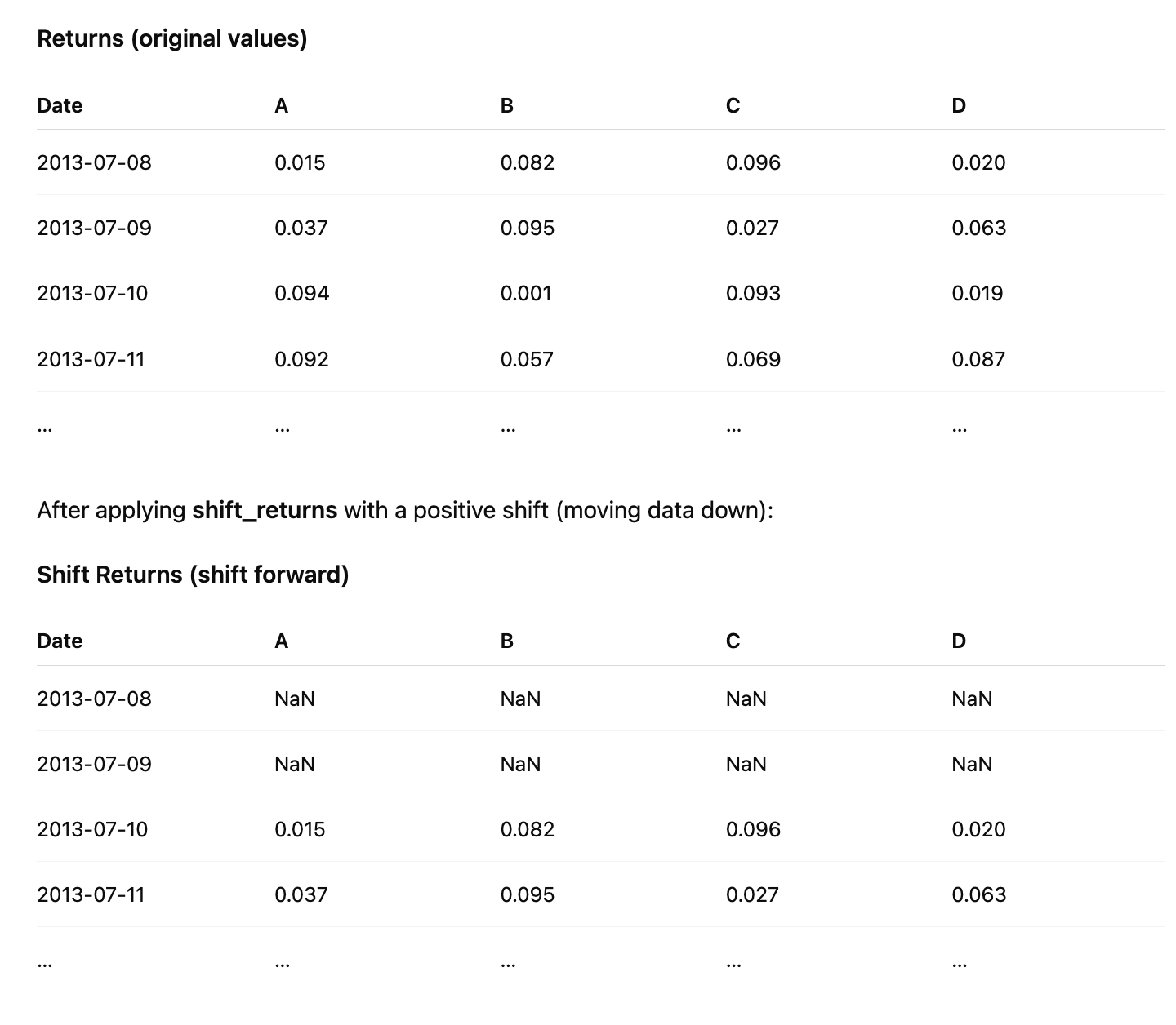
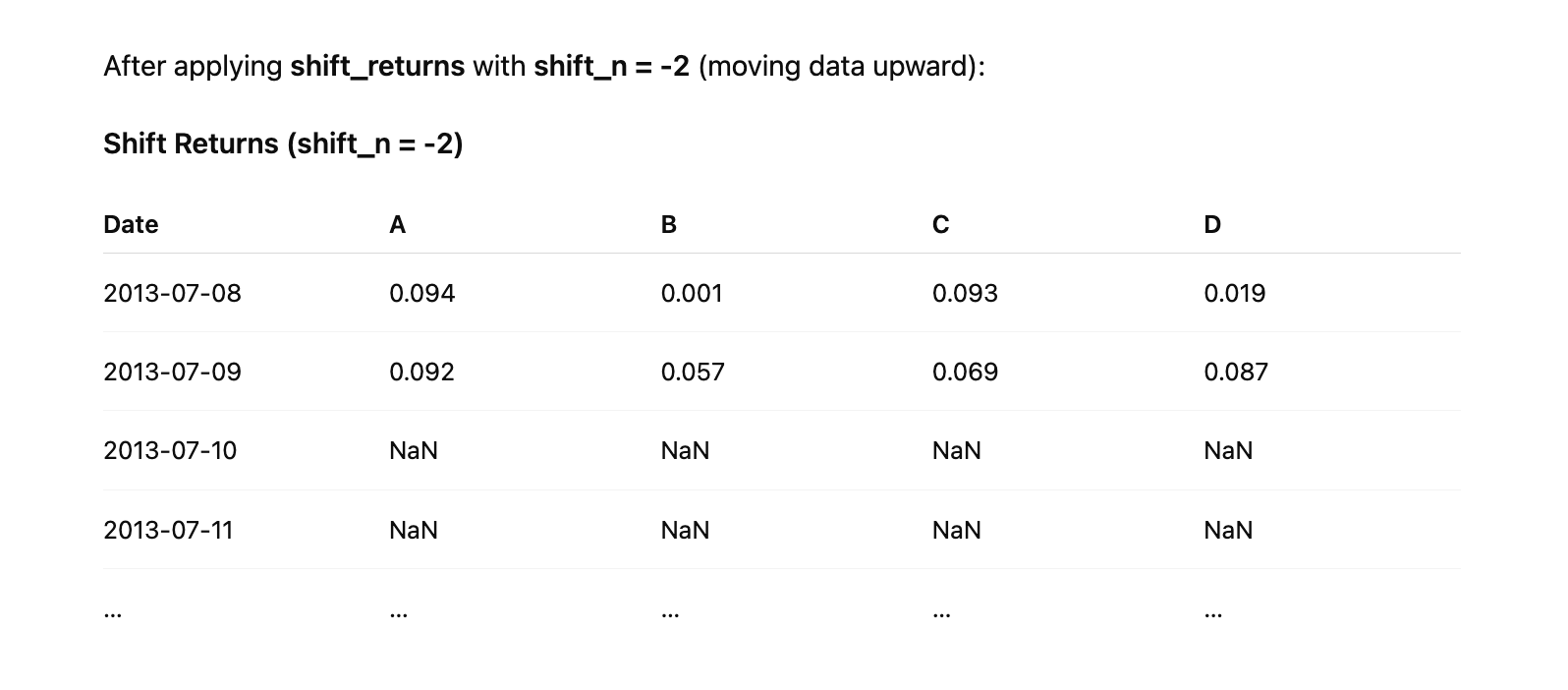
A positive shift moves the values downward in time and fills the top rows with NaN, while a negative shift moves the values upward and fills the bottom rows with NaN.
def shift_returns(returns, shift_n):
    “”“
    Generate shifted returns

    Parameters
    ----------
    returns : DataFrame
        Returns for each ticker and date
    shift_n : int
        Number of periods to move, can be positive or negative

    Returns
    -------
    shifted_returns : DataFrame
        Shifted returns for each ticker and date
    “”“
    if shift_n == 0:
        return returns.copy()
    output_df = pd.DataFrame(index=returns.index, columns=returns.columns)
    if shift_n > 0:
        output_df.iloc[shift_n:] = returns.iloc[:-shift_n]
    else:
        output_df.iloc[:shift_n] = returns.iloc[-shift_n:]
    return output_df
project_tests.test_shift_returns(shift_returns)
The shift_returns function is designed to shift the returns data in a DataFrame by a specified number of periods, which is essential in momentum trading strategies where historical returns need to be aligned with future periods to identify momentum signals — such as using past performance to forecast subsequent price movements. It begins by checking if shift_n is zero; in this case, no shift is required, so it returns a copy of the input returns DataFrame to preserve the original data without modification, ensuring that the function handles the trivial case efficiently while avoiding unnecessary operations.
For non-zero shifts, the function creates an empty output DataFrame with the same index and columns as the input returns, initializing it with NaN values by default. This setup maintains the structural integrity of the data — keeping the same tickers as columns and dates as rows — while preparing space to insert the shifted values, which is crucial for time-series analysis in momentum trading where the temporal alignment must remain consistent across assets.
If shift_n is positive, indicating a forward shift (e.g., to lag returns for predictive features), the function assigns the first portion of the original returns — specifically, returns.iloc[:-shift_n] — to the later rows of the output DataFrame starting from index shift_n. This effectively moves the data downward by shift_n periods, filling the initial rows with NaN to represent unavailable historical data, allowing momentum models to incorporate lagged returns without disrupting the overall DataFrame shape.
Conversely, if shift_n is negative, denoting a backward shift (e.g., to lead returns for outcome simulation), the function assigns the last portion of the original returns — returns.iloc[-shift_n:] — to the earlier rows of the output DataFrame up to index shift_n. This shifts the data upward by the absolute value of shift_n periods, populating the top rows with future returns while leaving the trailing rows as NaN, which supports evaluating momentum strategies by comparing shifted historical signals against actual subsequent performance.
In both shifting cases, the use of integer-location indexing (iloc) ensures precise row-level manipulation without altering the index labels, preserving the date-time integrity vital for momentum trading backtests. The resulting output_df thus provides a transformed view of returns that facilitates feature engineering, such as creating momentum indicators based on prior period gains or losses.
View Data
Retrieve the returns for the previous and next months.
apple_series = monthly_close_returns[apple_ticker]
project_helper.plot_shifted_returns(
    apple_series.shift(1),
    apple_series,
    f’Previous Returns of {apple_ticker} Stock’)
project_helper.plot_shifted_returns(
    apple_series.shift(-1),
    apple_series,
    f’Lookahead Returns of {apple_ticker} Stock’)
where historical price momentum is used to forecast future returns and inform buy or sell decisions, this code segment begins by isolating the time series of monthly closing returns for the Apple stock, specified by the apple_ticker variable, from a broader dataset stored in monthly_close_returns. This extraction creates a focused pandas Series, apple_series, containing the sequential monthly return values for Apple, enabling targeted analysis of its momentum characteristics without interference from other assets.
Next, the code invokes the plot_shifted_returns function from the project_helper module to visualize the relationship between lagged returns and the current returns, which is crucial for assessing how past performance influences present momentum in trading strategies. Specifically, it passes apple_series.shift(1) — which displaces the return series forward by one period, aligning each current return with the immediately preceding month’s return — as the first argument, alongside the unshifted apple_series as the second argument for comparison. The title, formatted as ‘Previous Returns of {apple_ticker} Stock’, labels the plot to highlight this backward-looking perspective. This setup allows the plot to illustrate the correlation between prior-period returns and subsequent ones, revealing momentum persistence where strong past gains (or losses) tend to continue, a core principle for timing entries and exits in momentum-based trades.
Finally, the code calls plot_shifted_returns again, but with apple_series.shift(-1) — which shifts the series backward by one period, effectively aligning each current return with the next month’s return — as the first argument, again paired with the original apple_series. Titled ‘Lookahead Returns of {apple_ticker} Stock’, this visualization demonstrates the hypothetical forward relationship between current and future returns. In momentum trading development, such a plot serves to explore potential predictive power by showing how today’s momentum might anticipate tomorrow’s performance, though in practice, it underscores the importance of avoiding lookahead bias in model training to ensure realistic backtesting and live strategy deployment. Through these sequential plots, the code facilitates a visual diagnostic of Apple’s return dynamics, aiding in the refinement of momentum signals for the overall trading system.
Generate Trading Signal
A trading signal consists of a sequence of trading actions or results that guide trading decisions. A common approach generates long and short portfolios of stocks at regular intervals, such as the end of each month, based on your desired trading frequency. You can interpret this signal as a directive to rebalance your portfolio on those dates, entering long (buy) and short (sell) positions as specified.
The following strategy ranks stocks by their previous returns at the end of each month, from highest to lowest. It selects the top performers for the long portfolio and the bottom performers for the short portfolio.
For each month-end observation period, rank the stocks by previous returns, from highest to lowest. Select the top-performing stocks for the long portfolio and the bottom-performing stocks for the short portfolio.
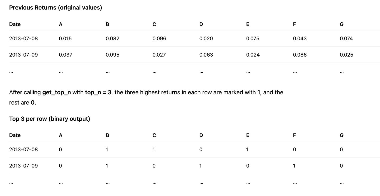
Implement the get_top_n function to identify the top-performing stocks for each month. For the top n stocks in prev_returns, assign a value of 1; assign 0 to all others. For example, given the following prev_returns:
def get_top_n(prev_returns, top_n):
    “”“
    Select the top performing stocks

    Parameters
    ----------
    prev_returns : DataFrame
        Previous shifted returns for each ticker and date
    top_n : int
        The number of top performing stocks to get

    Returns
    -------
    top_stocks : DataFrame
        Top stocks for each ticker and date marked with a 1
    “”“
    indicator_matrix = pd.DataFrame(0, index=prev_returns.index, columns=prev_returns.columns)

    print(indicator_matrix.head())

    yield_mapping = prev_returns.to_dict(’index’)

    for timestamp, performance_dict in yield_mapping.items():
        leading_performers = sorted(performance_dict.items(), key=lambda item: item[1], reverse=True)[:top_n]
        for symbol, _ in leading_performers:
            indicator_matrix.loc[timestamp, symbol] = 1

    print(indicator_matrix)
return indicator_matrixproject_tests.test_get_top_n(get_top_n)the get_top_n function plays a crucial role by identifying the highest-performing stocks from historical returns data, allowing us to focus investment decisions on assets exhibiting strong upward momentum. This selection process ensures that our portfolio prioritizes stocks with the best recent performance, which is a core principle of momentum trading to capitalize on trends continuing in the short term.
The function begins by initializing an indicator matrix as a DataFrame filled with zeros, using the same index (typically timestamps) and columns (stock symbols) as the input prev_returns DataFrame. This matrix serves as a binary selector: positions will remain zero for underperforming stocks and flip to one for the top performers, enabling downstream logic to easily filter and weight allocations toward momentum leaders. By starting with zeros across all entries, we create a clean slate that systematically marks only the qualifying stocks, avoiding any bias from prior computations.
Next, the function converts the prev_returns DataFrame into a dictionary where each key is a timestamp from the index, and the value is a dictionary of stock symbols mapped to their respective returns at that time. This restructuring facilitates efficient per-timestamp processing, as momentum evaluation in trading strategies often requires isolating performance snapshots to rank stocks independently for each period, ensuring that selections reflect contemporaneous market conditions rather than cross-temporal influences.
For each timestamp in the dictionary, the code sorts the inner performance dictionary’s items — pairs of stock symbols and their returns — in descending order based on the return values. It then slices the top top_n entries from this sorted list, capturing the leading performers whose positive momentum justifies inclusion in our trading signals. This sorting and selection step is essential because it quantifies momentum by directly comparing returns, allowing the strategy to dynamically adapt to varying market leadership without fixed thresholds, which could miss nuanced shifts in performance hierarchies.
For each selected stock symbol from the top performers at that timestamp, the function updates the corresponding position in the indicator matrix to 1 using row-column indexing. This targeted assignment creates a sparse yet precise representation of our momentum picks: only the highest-returning stocks per period are flagged, which streamlines portfolio construction by providing a ready-made mask for weighting or filtering in subsequent trading steps, such as position sizing or rebalancing.
Finally, the function prints the full indicator matrix for verification during development or debugging, offering a quick visual confirmation of the selection logic’s output, and returns the matrix itself. This output integrates seamlessly into the broader momentum trading pipeline, where it can be used to generate buy signals or allocate capital exclusively to these top-ranked stocks, thereby enforcing the strategy’s discipline in pursuing sustained price trends.
View Data
To identify the best and worst performing stocks, use the get_top_n function.
For the best performing stocks, pass prev_returns to the function.
For the worst performing stocks, pass -1 * prev_returns instead. This negation converts positive returns to negative values and negative returns to positive values, so get_top_n selects the stocks with the lowest original returns.
selection_count = 50
inverted_prev = prev_returns * -1
long_selection = get_top_n(prev_returns, selection_count)
short_selection = get_top_n(inverted_prev, selection_count)
for portfolio_type, data_frame in [(’Longed Stocks’, long_selection), (’Shorted Stocks’, short_selection)]:
    project_helper.print_top(data_frame, portfolio_type)
this code block focuses on selecting and displaying candidate stocks for long and short positions based on historical returns, aiming to capitalize on the persistence of price trends by identifying top performers and underperformers from prior periods. The process begins by defining a selection threshold of 50 stocks, which determines the size of each portfolio subset to ensure a focused yet diversified set of momentum signals without overwhelming computational resources. To prepare for short position selection, the previous returns data — assumed to be a DataFrame or array of stock performance metrics — is inverted by multiplying by -1; this transformation flips the return values so that the strongest negative performers (potential shorts) become the highest positive values, enabling a uniform top-selection mechanism across both strategies.
Next, the code applies a helper function, get_top_n, to extract the top 50 entries from the original previous returns, forming the long_selection. This step identifies stocks with the highest past returns, as momentum trading posits that these winners are likely to continue outperforming due to sustained investor interest and market inertia. Similarly, get_top_n is called on the inverted returns to produce the short_selection, which effectively captures the 50 stocks with the most negative original returns; by leveraging the inversion, the function ranks the biggest losers as “top” in the modified dataset, aligning with the strategy’s goal of shorting assets expected to decline further based on recent downward momentum.
Finally, the code iterates over a list of tuples pairing descriptive portfolio types with their respective selections — ‘Longed Stocks’ with long_selection and ‘Shorted Stocks’ with short_selection. For each pair, it invokes project_helper.print_top to output the ranked data, providing a clear visualization of the momentum-based picks. This printing step facilitates quick review and validation of the selections, ensuring the trading signals derived from past returns are transparently communicated for downstream decision-making in the momentum strategy.
Projected Returns
Now, evaluate whether your trading signal has the potential to generate profits.
Begin by calculating the net returns for this portfolio. For simplicity, assume an equal dollar investment in each stock. This approach allows you to compute the portfolio returns as the arithmetic average of the individual stock returns.
Implement the portfolio_returns function to calculate the expected portfolio returns. Use df_long to identify stocks for long positions and df_short for short positions, and compute the returns based on lookahead_returns. The variable n_stocks indicates the number of stocks invested in for a given period, which will assist with the calculations.
def portfolio_returns(df_long, df_short, lookahead_returns, n_stocks):
    “”“
    Compute expected returns for the portfolio, assuming equal investment in each long/short stock.

    Parameters
    ----------
    df_long : DataFrame
        Top stocks for each ticker and date marked with a 1
    df_short : DataFrame
        Bottom stocks for each ticker and date marked with a 1
    lookahead_returns : DataFrame
        Lookahead returns for each ticker and date
    n_stocks: int
        The number number of stocks chosen for each month

    Returns
    -------
    portfolio_returns : DataFrame
        Expected portfolio returns for each ticker and date
    “”“
    # TODO: Implement Function
    def calculate_net(row_l, row_s, row_f, count):
        multiplied_l = row_l * row_f
        multiplied_s = row_s * row_f
        difference = multiplied_l - multiplied_s
        return difference / count

    result_df = df_long.apply(
        lambda idx: calculate_net(
            df_long.loc[idx],
            df_short.loc[idx],
            lookahead_returns.loc[idx],
            n_stocks
        ),
        axis=1
    )

    return result_df
project_tests.test_portfolio_returns(portfolio_returns)
where the strategy involves going long on top-performing stocks (expected to continue outperforming) and short on underperforming ones (expected to continue lagging), this function computes the expected portfolio returns by simulating an equal-weighted position across the selected long and short stocks for each date and ticker. The process begins by defining an inner helper function, calculate_net, which takes row slices from the long selection DataFrame (df_long), short selection DataFrame (df_short), and lookahead returns DataFrame (lookahead_returns), along with the number of stocks selected per side (n_stocks). For a given row index — representing a specific date and ticker — the function first computes the element-wise product of the long row (a binary mask of 1s for selected long stocks and 0s elsewhere) with the corresponding lookahead returns row; this isolates and sums the forward-looking returns only for the long positions, effectively capturing the total return from longs under the assumption of equal investment. Similarly, it computes the element-wise product for the short row, summing the returns for short positions. The difference between these summed long and short returns represents the net directional exposure of the momentum portfolio — positive if longs outperform shorts, as anticipated in momentum strategies — before dividing by n_stocks to normalize for the equal weighting across the selected stocks on each side, yielding the average net return per stock position. This calculation ensures the portfolio return reflects the strategy’s core bet on momentum persistence without overweighting any individual stock.
The outer logic then applies this calculate_net function across all rows of df_long using pandas’ apply method with axis=1, which iterates sequentially over each row index (date-ticker combination) in df_long. For each such index, it retrieves the aligned row slices from df_long, df_short, and lookahead_returns via loc[idx], ensuring that the masks and returns are synchronized by date and ticker to avoid misalignment in the momentum signal. By applying the function row-wise, the code processes the entire dataset in a vectorized manner per row, producing a result Series (named result_df) indexed by the original row indices, where each value is the computed net portfolio return for that date-ticker pair. This output directly supports momentum trading evaluation by providing a time-series of expected portfolio performance, allowing backtesting or analysis of how the long-short spread captures momentum effects across periods. The function’s design assumes df_long and df_short have exactly n_stocks 1s per relevant row to maintain the equal-weighting premise, with the division by n_stocks ensuring the return is scaled appropriately for portfolio-level interpretation.
View Data
Examine the data to assess the portfolio’s performance.
portfolio_length = top_bottom_n * 2
prospective_investment_yields = portfolio_returns(df_long, df_short, lookahead_returns, portfolio_length)
consolidated_yields = prospective_investment_yields.sum(axis=1)
project_helper.plot_returns(consolidated_yields, ‘Portfolio Returns’)
this code block constructs and visualizes the overall portfolio returns by combining long and short positions to exploit price momentum trends. It begins by determining the total portfolio length as top_bottom_n * 2, where top_bottom_n represents the number of top-performing assets selected for long positions and an equal number of bottom-performing assets for short positions; this doubling ensures the portfolio balances equal-weighted exposure on both sides, capturing the full momentum signal across the selected extremes without overweighting one direction.
Next, the code invokes the portfolio_returns function, passing the long-position dataframe (df_long), short-position dataframe (df_short), lookahead returns (lookahead_returns), and the computed portfolio_length. This function calculates prospective investment yields by simulating the strategy’s performance: it evaluates how the momentum-selected long assets (expected to continue rising) and short assets (expected to continue falling) would contribute to returns over the lookahead period, aggregating these yields into a structured array where rows correspond to time steps and columns to individual positions, thereby quantifying the strategy’s potential profitability based on historical momentum patterns.
The resulting prospective_investment_yields array is then consolidated by summing along the axis=1 dimension, which aggregates the yields across all positions (both long and short) for each time step; this step derives the net portfolio return series, effectively netting out the opposing bets to isolate the pure momentum-driven alpha, as the strategy profits from the divergence between winners and losers rather than directional market moves.
Finally, the consolidated yields are passed to project_helper.plot_returns along with the label ‘Portfolio Returns’, generating a visualization that charts the cumulative or periodic returns over time; this plot serves to inspect the strategy’s historical backtested performance, highlighting periods of momentum persistence or reversal to validate the approach in our momentum trading framework.
Statistical Tests
Annualized Rate of Return
total_periodic_yields = expected_portfolio_returns.sum(axis=0).dropna()
yield_array = total_periodic_yields.values
central_tendency = np.mean(yield_array)
dispersion_measure = np.std(yield_array, ddof=1)
sample_size = len(yield_array)
error_estimate = dispersion_measure / np.sqrt(sample_size)
compounded_yearly = (np.exp(central_tendency * 12) - 1) * 100
print(”“”
Mean:                       {:.6f}
Standard Error:             {:.6f}
Annualized Rate of Return:  {:.2f}%
“”“.format(central_tendency, error_estimate, compounded_yearly))
this code block evaluates the performance of an expected portfolio by deriving essential statistical metrics from periodic yield data, enabling traders to gauge the strategy’s average profitability, variability, and precision over time. The process begins by aggregating the yields across the portfolio’s components: it sums the values in expected_portfolio_returns along the asset dimension (axis=0), which assumes the input is structured with rows representing assets and columns representing time periods, resulting in a series of total portfolio yields per period. Any missing values are then removed via dropna() to ensure the subsequent calculations operate on complete, reliable data, preventing distortions in the momentum strategy’s performance assessment.
Next, the aggregated yields are converted into a NumPy array (yield_array) for efficient numerical processing, as this format supports the vectorized operations needed for statistical computations. The central tendency of these periodic yields is calculated as the arithmetic mean (central_tendency), providing a summary measure of the average return generated by the momentum-based portfolio over the observed periods; this is crucial for understanding the baseline profitability that momentum signals aim to capture by buying assets with upward trends and selling those with downward ones.
To quantify the variability inherent in the momentum strategy’s returns — which can arise from market volatility or the timing of momentum reversals — the code computes the sample standard deviation (dispersion_measure) using ddof=1 to apply Bessel’s correction, yielding an unbiased estimate of the population standard deviation from the finite sample of periods. The sample size (sample_size) is then determined as the length of the yield array, which directly informs the reliability of these estimates in a trading context where historical periods represent the available evidence for strategy validation.
Building on this, the standard error (error_estimate) is derived by dividing the dispersion measure by the square root of the sample size, offering a measure of how precisely the mean return estimates the true underlying return of the momentum portfolio; a smaller error indicates greater confidence in the strategy’s consistent performance across periods, which is vital for risk-adjusted decision-making in momentum trading.
Finally, to contextualize the results for practical trading evaluation, the code annualizes the mean periodic return assuming monthly intervals: it applies continuous compounding via the exponential function on central_tendency multiplied by 12 (to scale to yearly), subtracts 1 to express it as a simple return, and multiplies by 100 for percentage formatting (compounded_yearly). This transformation allows traders to compare the momentum strategy’s projected yearly performance against benchmarks or risk thresholds. The metrics are then output in a formatted print statement, displaying the mean, standard error, and annualized rate to six or two decimal places as appropriate, facilitating quick interpretation of the portfolio’s expected behavior under momentum-driven allocations.
The annualized rate of return enables you to compare this strategy’s return rate with other rates, which are typically quoted on an annual basis.
T-Test
The null hypothesis (H0H0) states that the actual mean return from the signal is zero. To test this, perform a one-sample, one-sided t-test on the observed mean return and determine whether to reject H0H0.
First, compute the t-statistic and then determine its corresponding p-value. The p-value represents the probability of observing a t-statistic that is equally or more extreme than the one calculated, assuming the null hypothesis is true. A small p-value indicates a low probability of observing the calculated t-statistic under the null hypothesis, which casts doubt on H0H0. As a best practice, set the desired significance level, or αα, before computing the p-value, and then reject the null hypothesis if p<αp<α.
For this project, use α=0.05α=0.05, a common significance level.
Implement the analyze_alpha function to perform a t-test on the sample of portfolio returns. The scipy.stats module has been imported for this purpose.
from scipy import stats
from scipy.stats import t
def analyze_alpha(expected_portfolio_returns_by_date):
    “”“
    Perform a t-test with the null hypothesis being that the expected mean return is zero.

    Parameters
    ----------
    expected_portfolio_returns_by_date : Pandas Series
        Expected portfolio returns for each date

    Returns
    -------
    t_value
        T-statistic from t-test
    p_value
        Corresponding p-value
    “”“
    sample_size = len(expected_portfolio_returns_by_date)
    avg_return = expected_portfolio_returns_by_date.mean()
    sample_std = expected_portfolio_returns_by_date.std()
    hypothesized_mean = 0.0
    standard_error = sample_std / (sample_size ** 0.5)
    test_statistic = (avg_return - hypothesized_mean) / standard_error
    degrees_freedom = sample_size - 1
    two_tailed_p = 2 * t.cdf(-abs(test_statistic), degrees_freedom)
    one_tailed_p = two_tailed_p / 2
    return test_statistic, one_tailed_p
project_tests.test_analyze_alpha(analyze_alpha)
where the goal is to identify and capitalize on persistent price trends to generate excess returns (alpha) over a benchmark, the analyze_alpha function evaluates the statistical significance of a portfolio’s expected returns. It performs a one-sample t-test to assess whether the mean of these returns is significantly different from zero, which helps determine if the momentum strategy is producing reliable alpha rather than random noise. The function takes a Pandas Series of expected portfolio returns indexed by date as input, ensuring the analysis is grounded in time-series data typical of trading strategies.
The process begins by extracting key descriptive statistics from the input series to set up the t-test. The sample size is computed as the length of the series, providing the basis for degrees of freedom and error estimation. The average return is calculated as the mean of the series, representing the observed central tendency of the portfolio’s performance. The sample standard deviation is then derived, quantifying the variability in returns, which is crucial for understanding the uncertainty in the estimate of the mean. These steps prepare the data for hypothesis testing by summarizing its distribution, allowing us to evaluate if the observed average return deviates meaningfully from the null hypothesis of zero mean return — a benchmark implying no alpha generation in the momentum strategy.
Next, the function computes the standard error of the mean, defined as the sample standard deviation divided by the square root of the sample size. This measure scales the variability to the precision of the mean estimate, becoming smaller with larger samples to reflect increased confidence in the average return’s reliability for momentum trading decisions. The t-statistic is then calculated as the difference between the average return and the hypothesized mean of zero, divided by the standard error. This standardized score quantifies how many standard errors the observed mean is away from zero, enabling a direct assessment of the strategy’s performance strength relative to sampling variability.
To derive the p-value, the degrees of freedom are set to the sample size minus one, accounting for the estimation of the standard deviation from the data and ensuring the t-distribution used is appropriate for the sample’s finite size. The two-tailed p-value is computed using the cumulative distribution function (CDF) of the t-distribution: specifically, twice the CDF evaluated at the negative absolute value of the t-statistic with the given degrees of freedom. This approach captures the probability of observing a t-statistic as extreme or more extreme in both directions under the null hypothesis, providing a symmetric test for significance. Finally, the one-tailed p-value is obtained by halving the two-tailed value, focusing on the direction of positive alpha relevant to momentum trading, where we are primarily interested in whether returns exceed zero.
The function returns the t-statistic and the one-tailed p-value, offering concise outputs that can be used downstream to interpret the strategy’s effectiveness — for instance, a low p-value alongside a positive t-statistic would indicate strong evidence against the null, supporting the momentum approach’s ability to deliver statistically significant alpha.
View Data
Review the values generated by your portfolio. After running this, ensure you address the question that follows.
metrics = analyze_alpha(expected_portfolio_returns_by_date)
stat_t, prob_p = metrics
print(f”“”
Alpha analysis:
 t-value:        {stat_t:.3f}
 p-value:        {prob_p:.6f}
“”“)
The provided code snippet performs a focused statistical analysis on the alpha component of the portfolio returns, which is essential in momentum trading to quantify whether the strategy generates excess returns beyond what would be expected from market exposure alone. It begins by invoking the analyze_alpha function with the expected_portfolio_returns_by_date data structure, which contains time-series returns for the portfolio derived from momentum signals. This function executes a statistical test — typically a regression-based approach, such as regressing the portfolio returns against a benchmark like the market return — to estimate the alpha (intercept term representing abnormal performance) and compute its significance through a t-statistic and associated p-value. The t-statistic measures how many standard errors the estimated alpha deviates from zero, helping to assess the reliability of the alpha estimate, while the p-value indicates the probability that the observed alpha resulted from random chance rather than true skill in the momentum strategy.
The results from analyze_alpha are returned as a tuple and unpacked into stat_t for the t-value and prob_p for the p-value, enabling a direct evaluation of the strategy’s alpha significance without intermediate storage of the full metrics object. This unpacking ensures that only the key outputs needed for interpretation are isolated, streamlining the flow toward reporting in the context of momentum trading, where a high t-value and low p-value would signal a robust, non-zero alpha that justifies continuing or scaling the momentum-based positions.
Finally, the code outputs a formatted print statement displaying the t-value to three decimal places and the p-value to six decimal places, providing a concise summary of the alpha analysis. This presentation choice emphasizes precision for the p-value, as small values (e.g., below 0.05) are critical thresholds in hypothesis testing to reject the null hypothesis of zero alpha, thereby confirming the momentum strategy’s value in generating superior risk-adjusted returns over the analyzed period.
