


Navigating the Complexities of Algorithmic Trading: A Kaggle Challenge Analysis
Navigating the Complexities of Algorithmic Trading: A Kaggle Challenge Analysis
Insights and Innovations in Predicting Market Reactions to Liquidity Shocks"

In the intricate world of financial markets, predicting the impact of liquidity shocks on limit-order books stands as a formidable challenge. This article delves into an in-depth analysis of a 2011 Kaggle competition, where the goal was to develop sophisticated models capable of anticipating short-term market responses to these shocks. Utilizing a range of computational techniques, from Linear Regression to Random Forest Regression, the study explores various strategies to decode the elusive patterns of market movements. By dissecting the performance and intricacies of each model, this analysis not only offers valuable insights into algorithmic trading but also serves as a testament to the evolving landscape of financial data analysis.
The Link to the source code is at the end of this article.
In this analysis, the focus was on a Kaggle competition from 2011, now concluded, where the challenge was to create a model predicting the short-term effects of a liquidity shock on a limit-order book. A liquidity shock occurs when a trade alters the best bid or ask price. Liquidity in finance, often discussed but seldom defined, pertains to the capacity to swiftly trade large asset quantities at a low cost. It encompasses three aspects: spread, depth, and resiliency. The spread is the transaction cost for traders, depth indicates the market’s ability to handle large orders with minimal price impact, and resiliency, the temporal aspect, refers to how quickly a market’s spread and depth recover following a liquidity shock, which happens when a large trade consumes all available volume at one of the best prices. For further reference on this topic, see existing literature such as the work found in this academic paper.
The Kaggle competition centered on empirically modeling the book’s resiliency.
The analysis was conducted using AWS, utilizing S3 for data storage and SageMaker for processing. To start, dependencies must be set up, and the S3 bucket associated with the notebook instance must be specified. S3 serves for permanent data storage, while the local instance is for temporary storage. Regular cleanup of the local instance is advisable due to its limited memory.
Data output from the notebook is initially saved locally, then transferred to S3. Similarly, data input begins with fetching from S3 to the local instance before being loaded into the notebook.
Before proceeding, the following folder structure should be established in the S3 bucket, which will also be mirrored locally:
/data: This directory holds training and testing data, along with various model encodings. The competition dataset, renamed as kaggle_data.csv, should be stored here.
/models: This is where serialized models are kept, named in the format modelName_predict.model.
/predictions: This folder contains prediction templates and model predictions, named as modelName_predict.csv.
/testing: Here, individual price errors from each prediction are stored for analysis, in the format errors_modelName_predict.csv.
#Run this cell to setup dependencies
#MUST FILL IN BUCKETNAME BELOW

import boto3
import pickle
import pandas as pd
import numpy as np
import matplotlib.pyplot as plt
import matplotlib.dates as mdates
from sklearn import linear_model as lm
from sklearn import ensemble
from sklearn.model_selection import train_test_split
from datetime import datetime
from IPython.display import display

bucketName = "YOUR-BUCKET-NAME"
plt.style.use(['bmh'])
global dataPath_
dataPath_ = "data/"
global predictPath_
predictPath_ = "predictions/"
global modelsPath_
modelsPath_ = "models/"
global testingPath_
testingPath_ = "testing/"
global csvExt_
csvExt_ = ".csv"
global modelExt_
modelExt_ = ".model"

#assumes files are stored the same in s3 bucket as in local instance: same name and directory
def writeLocalToS3(path):
    with open(path,'rb') as f:
        return boto3.Session().resource("s3").Bucket(bucketName).Object(path).upload_fileobj(f)

def loadS3ToLocal(path):
    with open(path,'wb') as f:
        return boto3.Session().resource("s3").Bucket(bucketName).Object(path).download_fileobj(f)
This code first imports several dependencies that will later be used. The libraries depend on include libraries for data analysis and visualization, machine learning algorithms, and working with S3 buckets on AWS. The second is. After initializing a few global variables, we will define file paths, file extensions, and bucket names. The third. The writeLocalToS3 function takes a path to a local file, uses Boto3, a Python library for working with Amazon Web Services, to upload the file to AWS S3. The fourth step. A loadS3ToLocal function is also defined, which takes in a path for a local file and uses Boto3 to download the file from AWS S3. I. Please read: Later on in the code, this code will make use of these functions to transfer files between the local instance and the S3 bucket. In addition, In addition to explaining what each function does, the code also assumes that the files being stored in the S3 bucket have the same names and directory structures as the local files it references.
Dataset Overview
The dataset includes 754,018 instances of liquidity shocks across 102 securities traded on the London Stock Exchange. In the initial Kaggle competition, this dataset was exclusively used for training purposes, complemented by a distinct testing set for evaluating model submissions. However, the testing set is currently unavailable, necessitating the division of the original training dataset into two parts: one serving as test_data and the other as train_data.
kaggleData = "kaggle_data"
kaggleDataPath = dataPath_ + kaggleData + csvExt_

# loadS3ToLocal(kaggleDataPath)
full_data = pd.read_csv(kaggleDataPath)

unique_ids = full_data['security_id'].unique()
print("There are {} liquidity shocks across {} different securities".format(full_data.shape[0], len(unique_ids)))

full_data.head()
First, kaggleData is created and set equal to the text kaggle_data. A new variable kaggleDataPath is created by combining the variables dataPath_ and .csv in earlier code, kaggleData and .csv. By doing so, one is able to create a file path that points to a specific location where data is kept. The following line calls a function called loadS3ToLocal with the path created earlier as an argument. The function loads data from the specified location into the current environment. Data is read from the file path specified in kaggleDataPath and stored in the full_data variable using the pandas library. In the next line of code, we create an array of unique values from the security_id column in the full_data dataframe. After this array is created, unique_ids is assigned to it. As a final step, this code writes a message using the .format function to fill in the blanks with how many rows and unique values the full_data dataframe contains. In the full_data dataframe, the first five rows are displayed using the .head function.
Data Structure and Analysis Goal
Each dataset row represents a liquidity shock, comprising 100 events. These events are categorized as trades (where securities are bought or sold, momentarily collapsing the bid-ask spread to zero) or quotes (updates to the best bid or ask price). Although multiple quote events, and thus numerous liquidity shocks, are present in each row, the primary focus is on the trade occurring at event 49, which constitutes the central liquidity shock. Event 50 is a quote, showcasing the immediate market response to the shock.
The first 50 events in each row include four data points: best bid, best ask, timestamp, and transaction type (Trade or Quote). The latter 50 events (51–100) record only the best bid and best ask values. Additionally, each row is enriched with six other data elements:
security_id: A unique identifier for the security.
p_tcount: The total number of on-market trades for this security on the previous day.
p_value: The previous day’s total on-market notional value traded for this security, in pounds.
trade_vwap: The volume-weighted average price of the trade triggering the liquidity shock, in pence.
trade_volume: The size of the trade that caused the liquidity shock, quantified in the number of securities.
initiator: Indicator of whether the shock was initiated by a buyer (B) or seller (S).
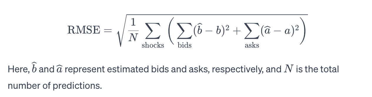
The analytical objective is to predict post-shock events (51–100) using the preceding information. The original competition assessed models based on the Root Mean Square Error (RMSE), calculated as follows:
fig, ax = plt.subplots(1)
full_data['security_id'].hist(bins=102)
fig.suptitle("Distribution of security_id field in the data", fontsize=16)
plt.show()
numSecurities = 3
topSecurities = (np.array(full_data['security_id']
.value_counts()
.sort_values(ascending=False)
.head(numSecurities).axes)).reshape(numSecurities)
print("Top {} securities: {}".format(numSecurities, topSecurities))
subset_data = full_data[full_data['security_id'].isin(topSecurities)]
unique_ids = subset_data['security_id'].unique()
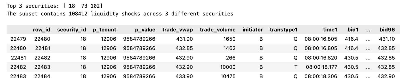
print("The subset contains {} liquidity shocks across {} different securities".format(subset_data.shape[0], len(unique_ids)))
subset_data.head()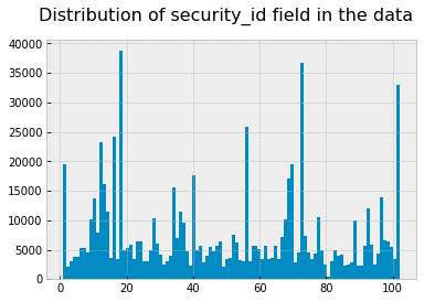
An snippet of code that visualizes and manipulates data. A breakdown of each line is as follows: — The first line creates a figure fig with a single subplot ax using the matplotlib library. Based on the full_data dataframe and 102 bins, the second line plots a histogram of the security_id column using the pandas library. A figure’s title appears on the third line. Figure 4 is shown on the fourth line. In the fifth line, we use the numpy library to create an array of the 3 most common security_id values. It prints a statement displaying the three top securities. A new subset_data is created with only rows in it whose security_id column matches one of the top three securities in the dataframe. A subset_data dataframe is created in line eight to contain unique security_id values. This statement prints the number of rows and unique securities in the dataframe subset_data on the ninth line. Data from the first five rows of subset_data are displayed in the tenth line.
The histogram presented illustrates a disparity in the representation of the 102 different securities within the dataset. To streamline the dataset for more efficient exploration, the analysis will be narrowed down to the three most frequently occurring securities. This approach still provides a substantial dataset, encompassing 108,412 instances of liquidity shocks for examination.
It’s important to note that the competition’s data collection process had a flaw resulting in the duplication of data for events 50 and 51 (where bid and ask prices for event 50 were identical to those of event 51). Consequently, to address this issue, the columns corresponding to event 51 will be excluded from the dataset. This adjustment means the analysis now focuses on predicting the outcomes of 49 events, specifically events 52 through 100.
subset_data = subset_data.drop('bid51', 1)
subset_data = subset_data.drop('ask51', 1)

subset_data.head()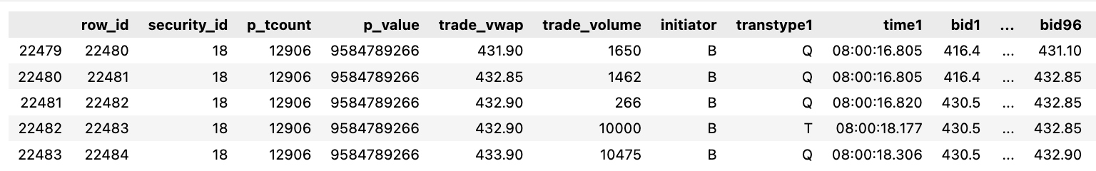
Subset_data is a DataFrame that has two columns, bid51 and ask51. This code removes them from the DataFrame. In the first line, the bid51 column is removed and in the second line, the ask51 column is removed. The number 1 indicates the axis along which the column should be removed. Column axis is the one in this case. DataFrame’s first five rows are simply printed in the last line.
The dataset will undergo a partitioning process where it is divided into training and testing subsets, following an 80%-20% split. To maintain a balanced representation of securities across both subsets, the sampling will be stratified based on the security_id. This ensures a consistent distribution of different securities in both the training and testing datasets. Additionally, to preserve the integrity of the testing data and avoid data leakage, the events designated for prediction in the testing set (events 52–100) will be omitted from it.
This strategy is crucial to ensure that a model is trained exclusively on the *train_data* and uses the *predict_data* for predictions, but is never exposed to the *test_data*. The test data, containing the actual outcomes, is reserved for a separate evaluation process to assess the model’s performance accurately.
trainDataPath = dataPath_ + "train_data" + csvExt_
testDataPath = dataPath_ + "test_data" + csvExt_
predictDataPath = predictPath_ + "predict_data" + csvExt_

stratifyLabel = subset_data['security_id'].values
train_data, test_data = train_test_split(subset_data, test_size=0.2, stratify=stratifyLabel)

train_data.to_csv(trainDataPath, index=False)
writeLocalToS3(trainDataPath)

test_data.to_csv(testDataPath, index=False)
writeLocalToS3(testDataPath)

print("The training data contains {} liquidity shocks".format(train_data.shape[0]))
print("The testing data contains {} liquidity shocks".format(test_data.shape[0]))

columnsToClear = []

for i in range(52,101):
    for column in test_data.columns.values:
        if column.endswith(str(i)) and (column.startswith("bid") or column.startswith("ask")):
            columnsToClear.append(column)

empty_predictions = pd.DataFrame( np.zeros((test_data.shape[0], len(columnsToClear))), index=test_data.index, columns=columnsToClear)
test_data.update(empty_predictions)

test_data.to_csv(predictDataPath, index=False)
writeLocalToS3(predictDataPath)

test_data.head()
In the first three lines, the file paths for training data, testing data, and prediction data are created by concatenating the file path with the corresponding file name. StratifyLabel is created by taking the security_id values from subset_data. A test size of 0.2 is used in the train_test_split function to split subset_data into train_data and test_data. This parameter ensures the data is split based on the same proportion of security_id values using the stratifyLabel variable. In addition to saving train_data and test_data as CSV files, the writeLocalToS3 function is also used for writing these files to the specified locations. The following two lines provide a count of rows in the train_data and test_data files, which correspond to the number of liquidity shocks. Another for loop iterates through the columns in test_data file within the for loop as it traverses 52 to 101 values. This means that if the column name ends with the outer loop value, then the loop value will be used. Columns whose names start with either bid or ask are added to the columnsToClear list. As a result, this list contains the column names of all bids and asks for the specified range of values. A new dataframe is created, empty_predictions, with the same number of rows as the test_data file and the same columns as columnsToClear. Dataframe filled with zeros for updating test_data file. A csv file of the updated test_data is saved at the specified path using the to_csv and writeLocalToS3 functions. Finally, the head method is used to print the first few rows of the test_data file.
Data Exploration Phase
The next step involves delving into the training data to gain insights into potential features that could effectively predict the state of the order book following a liquidity shock. The upcoming analysis will use code modified from a previous source, designed specifically to visualize and understand the dynamics of the order book.
def PlotShock(dataPath, row_id):

    loadS3ToLocal(dataPath)
    data = pd.read_csv(dataPath)

    bid_column_names = []
    ask_column_names = []
    for column in data.columns.values:
        if column.startswith('bid'):
            bid_column_names.append(column)
        elif column.startswith('ask'):
            ask_column_names.append(column)

    event_stamps = range(1,100)
    row = data.loc[ data['row_id']==row_id, : ]
    bid_values = np.array(row[bid_column_names]).flatten('F')
    ask_values = np.array(row[ask_column_names]).flatten('F')

    plt.figure(figsize=(10,8))

    plt.plot(event_stamps, ask_values, label='ask', color='b')
    plt.plot(event_stamps, bid_values, label='bid', color='g')

    x0, x1, y0, y1 = plt.axis()
    plt.axis((x0 - 0.25,
              x1 + 0.25,
              y0 - 0.25,
              y1 + 0.25))

    plt.axvline(x=49, color='r', linestyle='--')

    plt.fill_between(event_stamps, ask_values, ask_values*10, interpolate=True, color='b', alpha=0.3)
    plt.fill_between(event_stamps, 0, bid_values, interpolate=True, color='g', alpha=0.3)

    plt.xlabel("Event No")
    plt.ylabel("Best Prices")

    plt.legend()
    plt.title("Limit Order Book")
    plt.show()

    display(row)
PlotShock is a function defined in line one of the code that takes two parameters, dataPath and row_id. CSV files can be plotted using this function. This line calls the function loadS3ToLocal, which loads the data from S3 to the local system. Thirdly, the read_csv function from the pandas library is used to read the data from the specified dataPath into a dataframe. As a result, the following two lines create empty lists named bid_column_names and ask_column_names. It is intended to store the column names beginning with bid and ask in these lists. Line 8 uses the startswith function to determine if the column name begins with bid or ask as it iterates through the columns in the dataframe. Names are added to the appropriate list if they match. On the following line, a variable event_stamps is created and assigned values from 1 to 100. In line 11, the loc function is used to select the row of data based on the specified row_id. Assigned to variable row is this row. The following two lines create new variables bid_values and ask_values by matching the names of the columns in bid_column_names and ask_column_names with loc. In the next step, these values are flattened using the numpy library’s flatten function. By using the figure function of matplotlib’s library, the code creates a new figure with a size of 10x8 inches. This code plots the ask_values and bid_values on the figure as blue and green lines, respectively. By adjusting lines 16–17, the axis limits of the figure are better matched to the data. A red dashed line style is added to the vertical line at x=49 using the axvline function on line 18. Lines 19–20 use the fill_between function to fill the area between the ask_values and ask_values*10 and between 0 and bid_values with a translucent blue and green color respectively. A legend, axis labels, and a title are added to the figure before it is displayed using the show command. This last line displays the selected row of data that was plotted in the figure using the display function.
trainDataPath = dataPath_ + "train_data" + csvExt_
PlotShock(trainDataPath, 226374)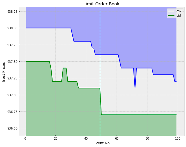

In the first line, trainDataPath is created and given a value that consists of dataPath_, train_data, and csvExt_. Strings can be concatenated together with the + operator. A second line calls PlotShock with two arguments: trainDataPath created in the first line and 226374. With this code snippet, a shock will be plotted from a CSV file at the specified path, which is constructed using the dataPath_ and csvExt_ variables. For a better understanding of how this code snippet works, it must be examined in detail.
The graph displays the dynamics of the order book for a specific liquidity shock (identified by row_id = 226374) involving security number 102. The shock was triggered by a sell trade, which absorbed all available volume at the best bid price, approximately 937.10. This transaction resulted in a decrease in the best bid price to around 936.70, causing a significant increase in the spread. In the subsequent events, the best bid price remained stable, while the best ask price gradually decreased until the spread almost reverted to its value before the shock.
It’s important to note that this pattern of mean reversion in the spread post-shock is not a consistent occurrence. Sometimes, a liquidity shock can lead the order book to settle into a new equilibrium state. Additionally, even in cases where the spread does revert to its original range, it is not always through the movement of the opposite best price. In this instance, the best ask price decreased to close the gap. However, in other scenarios, the best bid might increase, or both the best bid and ask could adjust in tandem to restore the spread to its previous state.
Benchmark Model
The simplest model is to predict constant bid and ask values that are equal to their values just after the shock (bid50 and ask50). We can use this as a benchmark on which to build more complexity.
def BenchmarkPredict():

    predictTemplatePath = predictPath_ + "prediction_data" + csvExt_
    modelPredictPath = predictPath_ + "benchmark_predict" + csvExt_

    loadS3ToLocal(predictTemplatePath)
    prediction_data = pd.read_csv(predictTemplatePath)

    bidColumnsToUpdate = []
    askColumnsToUpdate = []

    for i in range(52,101):
        for column in prediction_data.columns.values:
            if column.endswith(str(i)):
                if column.startswith('bid'):
                    bidColumnsToUpdate.append(column)
                if column.startswith('ask'):
                    askColumnsToUpdate.append(column)

    #for each liquidity shock
    for ix, row in prediction_data.iterrows():

        constBid = row['bid50']
        constAsk = row['ask50']

        #for each post-liquidity prediction
        for bidColumn in bidColumnsToUpdate:
            prediction_data.set_value(ix, bidColumn, constBid)
        for askColumn in askColumnsToUpdate:
            prediction_data.set_value(ix, askColumn, constAsk)

    prediction_data.to_csv(modelPredictPath, index=False)
    writeLocalToS3(modelPredictPath)

    display(prediction_data.head())
In this code snippet, BenchmarkPredict is defined. It creates two variables, predictTemplatePath and modelPredictPath, which contain path names of specific files. After that, the function calls loadS3ToLocal with predictTemplatePath as an argument. There is a good chance that this function loads data from a remote server S3 to a local machine. A variable named prediction_data is created by reading data from the predictTemplatePath file using the pandas library. We create two empty lists next, bidColumnsToUpdate and askColumnsToUpdate. Using a for loop, the prediction_data dataframe is iterated through each column name from 52 to 100. Whenever the column name ends with loop number i, it checks whether it starts with bid or ask, and if it does, it adds it to the appropriate list, bidColumnsToUpdate or askColumnsToUpdate. Afterward, a new for loop is added that repeats each row and index within prediction_data. This loop stores the current bid price in the bid50 column in the constBid variable and the current ask price in the constAsk variable. Iterate through the bidColumnsToUpdate and askColumnsToUpdate lists, setting each column’s value to the constant for the current row ix in two nested for loops. The constant values for each row are updated with the bid and ask columns. By using the writeLocalToS3 function, the updated prediction_data dataframe is also written to the remote server using the modelPredictPath file. The function displays the first five rows of the updated prediction_data dataframe. With this code snippet, we are creating a function to load data from a remote server, update certain columns with consistent values, and save the updated data to a new file which we write back to the remote server as well.
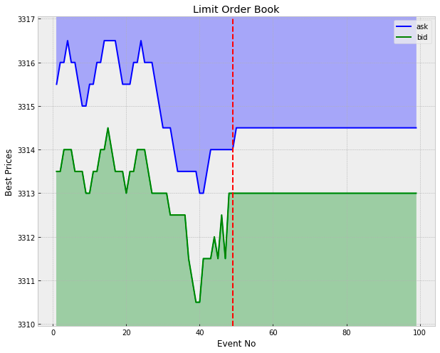
The plot above illustrates this simple model for a particular liquidity shock.
def RMSE( predictionData ):

    predictionDataPath = predictPath_ + predictionData
    testDataPath = dataPath_ + "test_data" + csvExt_
    predictTemplatePath = predictPath_ + "prediction_data" + csvExt_
    errorsPath = testingPath_ + "errors_" + predictionData

    loadS3ToLocal(predictionDataPath)
    prediction_data = pd.read_csv(predictionDataPath)

    loadS3ToLocal(testDataPath)
    results_data = pd.read_csv(testDataPath)

    loadS3ToLocal(predictTemplatePath)
    square_errors_data = pd.read_csv(predictTemplatePath)

    columnsToTest = []

    for i in range(52,101):
        for column in prediction_data.columns.values:
            if (column.endswith(str(i)) and (column.startswith("bid") or column.startswith("ask"))):
                columnsToTest.append(column)

    numPredictionsPerShock = len(columnsToTest)
    totalPredictions = numPredictionsPerShock * prediction_data.shape[0]
    sumSquaredErrors = 0.0

    #for each liquidity shock
    for ix, row in prediction_data.iterrows():

        print("Evaluating row: {}/{}".format(ix+1, prediction_data.shape[0]))

        row_id = row['row_id']

        predictedRow = prediction_data.loc[ prediction_data['row_id']==row_id, columnsToTest ]
        actualRow = results_data.loc[ results_data['row_id']==row_id, columnsToTest ]
        squareErrors = (predictedRow - actualRow)**2
        square_errors_data.loc[results_data['row_id']==row_id, columnsToTest] = squareErrors
        sumSquaredErrors += squareErrors.sum(axis=1).values[0]

    RMSE = np.sqrt( sumSquaredErrors / totalPredictions )

    square_errors_data.to_csv(errorsPath, index=False)
    writeLocalToS3(errorsPath)

    print("RMSE: {}".format(RMSE))
This code defines a function called RMSE that takes in an input called predictionData. Prediction data paths, test data paths, prediction template paths, and error paths are created using the defined variables: predictPath_, csvExt_, testingPath_, and dataPath_. The function then calls three functions: loadS3ToLocal with the predictionDataPath as an argument, pd.read_csv with the predictionDataPath as an argument, and square_errors_data with the predictTemplatePath. To load and read data from the given paths, these functions are used. Following that, the code creates a list called columnsToTest and uses a for loop to iterate over the range of numbers 52–101. This loop includes another for loop that iterates over the columns in the prediction data to determine if each column ends with the current number in the outer loop and begins with bid or ask. An appended column is added to the columnsToTest list if the condition is met. Using the columnsToTest list, the code calculates the number of predictions per shock by multiplying the column length by the number of rows in the prediction data. A variable called sumSquaredErrors, which stores the sum of squared errors, is initialized to 0.0 next. The next step is to iterate over the prediction data using the iterrows function. The code prints a progress message and assigns the row_id value to a new variable called actualRow for each row. In order to extract the predicted and actual rows from the prediction and results data, this actualRow variable must be set to the actualRow value. A squared error is calculated by subtracting the predicted row from the actual row and squaring the result. A square_errors_data dataframe is created to store these squared errors. RMSE is calculated by taking the square root of the sumSquaredErrors variable, dividing it by the total number of predictions, and then adding them together. In the square_errors_data dataframe, the RMSE value is then printed and saved. A CSV file is created in the square_errors_data dataframe, and the writeLocalToS3 function is used to upload the file to S3. The code snippet reads, manipulates, and calculates an RMSE for a given set of data by first defining a function and then using a series of functions and loops.
def PlotErrorsAgainstEvent( errorsData ):

    errorDataPath = testingPath_ + errorsData

    loadS3ToLocal(errorDataPath)
    errors_data = pd.read_csv( errorDataPath )

    bidColumns = []
    askColumns = []
    bidMeanSquareErrors = []
    askMeanSquareErrors = []

    for i in range(52,101):
        for column in errors_data.columns.values:
            if column.endswith(str(i)):
                if column.startswith('bid'):
                    bidColumns.append(column)
                if column.startswith('ask'):
                    askColumns.append(column)

    for column in bidColumns:
        bidMeanSquareErrors.append( errors_data.loc[:, column].mean() )

    for column in askColumns:
        askMeanSquareErrors.append( errors_data.loc[:, column].mean() )

    meanSquareErrors = np.array(bidMeanSquareErrors) + np.array(askMeanSquareErrors)

    predictionEvents = range(52, 101)
    plt.plot(predictionEvents, meanSquareErrors)

    plt.xlabel("Event No")
    plt.ylabel("Average Square Error")

    plt.title("A plot showing average square error as a function of time after the liquidity shock")
    plt.show()
A liquidity shock is shown as a function of time with the following code snippet. It works as follows: 1. An errorsData parameter is defined for the function. The path to the plotted errors data is specified by this parameter. The second is. Using errorsData as a parameter, the errorDataPath variable is created by concatenating the path to testing data with the testingPath_ variable. In addition, Loading data into a local file is performed by the loadS3ToLocal function. The fourth point. By reading the data from the local file into a pandas dataframe, the errors_data variable is created. I. Conclusion Next, four lines of code initialize lists that store column names and mean square errors. I. 6.5. For loops are used to iterate through the numbers 52 to 101, representing the predictions. The seventh. In the errors_data dataframe, another for loop is used to iterate through the column names. The eighth point. If the current column begins with either bid or ask, then the if statement checks if it ends with the prediction event number. The column name is added to the corresponding list bidColumns or askColumns if both conditions are met. In Number 9, In the second for loop, the mean function of the pandas dataframe is used to calculate mean square error for each column in the bidColumns list. Approximately ten. In the askColumns list, the same applies. 10.5 In Numpy, the bidMeanSquareErrors and askMeanSquareErrors lists are turned into arrays using the np.array function. In 2012 By adding these two arrays together, you obtain the meanSquareErrors array. The thirteenth. In order to create the predictionEvents variable, the range function is used to generate a list from 52 to 101. p.16. With plt.plot, the prediction events are plotted against the mean square errors. The 15th. Plot.show is used to display the plot’s labels and title, as well as add a label to the plot.
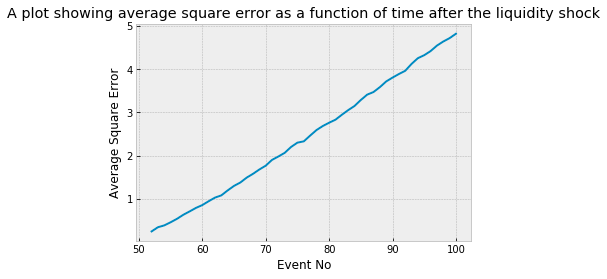
Though perhaps intuitive, the plot above highlights that the predictive power of our model decreases the further we move from the liquidity shock. The near perfect linearity is a surprise though. The average square error can be thought of as the variance of the security price after the shock, hence the standard deviation grows approximately like the square-root-of time: evidence of an underlying Geometric Brownian process.
def PlotErrorsAgainstPrice( errorsData ):

    errorDataPath = testingPath_ + errorsData

    loadS3ToLocal(errorDataPath)
    errors_data = pd.read_csv( errorDataPath )

    securityToFairPrices = {18:[], 73:[], 102:[]}
    securityToMeanSquareErrors = {18:[], 73:[], 102:[]}
    securityToColor = {18:'red', 73:'green', 102:'blue'}

    columnsToTest = []
    for i in range(52,101):
        for column in errors_data.columns.values:
            if (column.endswith(str(i)) and (column.startswith("bid") or column.startswith("ask"))):
                columnsToTest.append(column)

    for ix, row in errors_data.iterrows():
        security = row['security_id']
        fairPrice = (row['bid1'] + row['ask1'])/2
        securityToFairPrices[security].append(fairPrice)
        squareErrors = row.loc[columnsToTest]
        securityToMeanSquareErrors[security].append( squareErrors.mean() )

    fig, ax = plt.subplots()

    for security, fairPrices in securityToFairPrices.items():
        ax.scatter(fairPrices, securityToMeanSquareErrors[security], c=securityToColor[security], label=security)

    ax.legend()
    ax.set_xlabel("Initial Fair Price")
    ax.set_ylabel("Average Square Error")
    plt.title("A plot showing average square error as a function of initial fair price for each security considered.")
    plt.show()
In this code snippet, there is a function named PlotErrorsAgainstPrice, which takes in a parameter known as errorsData. During the first line of the function, a variable named errorDataPath will be created, which is defined as testingPath_ concatenated with errorsData. After calling loadS3ToLocal, the errorDataPath variable is passed into the function. Using this function, you can pull data from S3 and store it on your computer. On the following line, an errorDataPath variable is created and the output of the pd.read_csv function is assigned to errors_data. It reads data from a CSV file and creates a Pandas dataframe from it. Next, three dictionaries are created, namely securityToFairPrices, securityToMeanSquareErrors, and securityToColor. Using these, we will be able to store data related to each security. Using the next line, we create an empty list named columnsToTest. In this list, specific columns from error_data data frame will be stored. Iteration 52 to 101 is included in the first for loop. There are a number of columns in the errors_data dataframe that are accessed by this loop. Nested for loops iterate over the errors_data dataframe and check whether a column is named bid or ask and ends with i. It is added to the columnsToTest list if these conditions are met. In the following code, the iterrows function is used to loop through each row of the errors_data dataframe. A security_id and a fairPrice value are extracted from each row and stored in variables named security and fairPrice. Next, an error_data dataframe is created with the columnToTest list and a variable named squareErrors is created by using the loc function. The result is then added to the securityToMeanSquareErrors dictionary under the corresponding security value. In the final part of the code, a scatter plot is created using matplotlib on the created data. In the first line, a figure and axis are created using the subplots function. A for loop is then used to iterate over each security in securityToFairPrices. A scatter plot is created for each security based on its fairPrices and mean square errors. Each security’s color is determined by the securityToColor dictionary. Plot.show is used to display the plot using the x and y axes labels, the plot title, and the plot.show function.
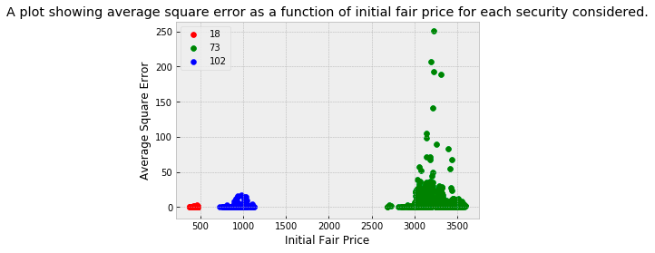
The three securities under examination each operate within distinct price brackets, with security 18 at the lower end and security 73 at the higher end of the range. The displayed plot reveals that the prediction error tends to be greater for securities trading at higher prices. This trend is somewhat expected given the nature of the Root Mean Square Error (RMSE) as the chosen error metric. Notably, a significant portion of the overall error can be attributed to a few liquidity shocks involving security 73. Adopting an error metric that considers errors as a fraction of the fair price could potentially mitigate this effect, leading to a more balanced error assessment across securities with varying price levels.
def PlotErrorsAgainstTime( errorsData ):

    errorDataPath = testingPath_ + errorsData

    loadS3ToLocal(errorDataPath)
    errors_data = pd.read_csv( errorDataPath )

    securityToShockTimes = {73:[], 102:[], 18:[]}
    securityToMeanSquareErrors = {73:[], 102:[], 18:[]}
    securityToColor = {18:'red', 73:'green', 102:'blue'}
    timeFormat = "%H:%M:%S.%f"
    marketOpen = "08:00:00.0"
    openDateTime = datetime.strptime(marketOpen, timeFormat)
    marketClose = "16:30:00.0"
    closeDateTime = datetime.strptime(marketClose, timeFormat)
    hours = mdates.HourLocator(interval = 1)
    h_fmt = mdates.DateFormatter('%H')

    columnsToTest = []
    for i in range(52,101):
        for column in errors_data.columns.values:
            if (column.endswith(str(i)) and (column.startswith("bid") or column.startswith("ask"))):
                columnsToTest.append(column)

    for ix, row in errors_data.iterrows():
        security = row['security_id']
        shockTime = datetime.strptime(row['time50'], timeFormat)
        securityToShockTimes[security].append( shockTime )
        squareErrors = row.loc[columnsToTest]
        securityToMeanSquareErrors[security].append( squareErrors.mean() )

    fig, ax = plt.subplots()

    for security, shockTimes in securityToShockTimes.items():
        ax.scatter(shockTimes, securityToMeanSquareErrors[security],
                   c=securityToColor[security], label=security, alpha=0.3)

    ax.legend()
    ax.set_xlim(openDateTime, closeDateTime)
    ax.xaxis.set_major_locator(hours)
    ax.xaxis.set_major_formatter(h_fmt)
    ax.set_xlabel("Time of Liquidity Shock")
    ax.set_ylabel("Average Square Error")
    plt.title("A plot showing average square error as a function of shock time.")
    plt.show()
The code snippet creates a function called PlotErrorsAgainstTime that receives a parameter called errorsData and initializes three dictionaries for storing errors, shock times, mean square errors, and security colors. Next, it creates datetime objects for the opening and closing times of the market. As a next step, it iterates through the error dataframe to add column names that are applicable to the test. Afterward, it iterates through each row in the dataframe and adds shock time and mean square error data. Lastly, it creates a scatter plot for each security showing shock times and mean square errors. Before the plot is displayed to the user, it is formatted with labels and titles.
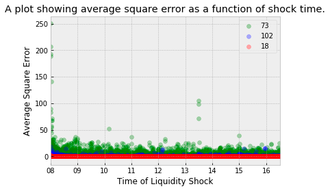
The plot demonstrates that prediction errors are not evenly distributed throughout the trading day. Notably, the market opening time is marked by high volatility, which adversely affects the performance of our model. Additionally, there’s a notable increase in errors around 13:30 UK time, coinciding with the 08:30 opening of the New York Stock Exchange (NYC time).
When this observation is combined with insights from the previous plot, it becomes evident that a significant portion of the total error is due to a few liquidity shocks in security 73, predominantly occurring around the market opening. This pattern can be attributed to two main factors: the RMSE metric, which tends to penalize higher-priced securities more heavily, and the model’s suboptimal performance during periods of high market volatility.