

Neural Network From Scratch To Mater
Units (also called nodes or neurons) are at the heart of neural networks.

A unit takes one or more inputs, multiplies each input by a parameter (also called a weight), sums the weighted inputs plus a bias value (typically 0), then feeds the value into an activation function. In the case of a neural network with other neurons (if there are any), the output is then sent to them.
Multilayer perceptrons, also known as feedforward neural networks, are the simplest artificial neural networks used in real-world settings. A neural network is composed of a series of interconnected layers that connect the feature values of an observation to the target value (for example, the observation’s class). The name feedforward comes from the fact that the feature values of an observation are fed “forward” through the network, with each layer transforming the feature values until the final output equals that of the target.
There are three types of layers in feedforward neural networks. Each unit in the neural network contains the value of an observation for a single feature in the input layer. An observation with 100 features has 100 nodes in the input layer. Output layers transform the hidden layers’ output into useful values at the end of a neural network. A sigmoid function can be used in our output layer to scale its own output to a predicted class probability of 0 or 1, for example, if our goal is binary classification. The “hidden” layers (which aren’t really hidden) sit between the input and output layers. Once the output layer processes the feature values from the input layer, the output layer transforms them into something that resembles the target class. The application of deep learning uses neural networks with multiple hidden layers (e.g., 10, 100, 1,000).
The parameters of a neural network are typically initialized as small random values from a Gaussian or normal uniform distribution. A loss function is used to compare the outputted value of the network with the observation’s true value after an observation (or more often a batch) has been fed through the network. Forward propagation is the process of doing this. As a next step, an algorithm goes “backward” through the network, identifying which parameters contributed most to the difference between the predicted and true values. Each weight is adjusted according to how much the optimization algorithm determines for each parameter.
For each observation in the training data, neural networks repeat the process of forward propagation and backpropagation multiple times in order to learn (epochs are the number of times all observations are sent through a network, and training typically consists of multiple epochs), adjusting the parameters iteratively.
To build, train, and evaluate neural networks, we will use the popular Python library Keras. It uses other libraries such as TensorFlow and Theano as its “engine.” For us, Keras has the advantage of allowing us to focus on training and network design rather than tensor operations.
CPUs (such as your laptop) and GPUs (such as specialized deep learning computers) can be used to train neural networks created using Keras code. For real-world use, neural networks should be trained on GPUs; however, the neural networks in this article can be trained on your laptop in just a few minutes for the sake of learning. Using CPUs is significantly slower than using GPUs when we have larger networks and more training data.
Using neural networks to preprocess data
In order to use a neural network, you need to preprocess data.
The following steps can be followed to standardize each feature using the scikit-learn StandardScaler:

Output:array([[-1.12541308, 1.96429418],[-1.15329466, -0.50068741],[ 0.29529406, -0.22809346],[ 0.57385917, -0.42335076],[ 1.40955451, -0.81216255]])While this snippet is very similar to snippet 4.3, its importance for neural networks makes it worth repeating. Small random numbers are typically used as initialization parameters for neural networks. When feature values are much larger than parameter values, neural networks tend to behave poorly. The scale of all features must also be the same since an observation’s features are combined as they pass through individual units.
Thus, standardizing each feature such that it has a mean of 0 and a standard deviation of 1 is best practice (although not always necessary). A simple way to do this is to use scikit-learn’s StandardScaler.
By checking our first feature’s mean and standard deviation, you can see the effect of standardization:

Output:Mean: 0.0Standard deviation: 1.0Designing a Neural Network
You want to design a neural network? Let’s do it!
Use Keras’ Sequential model:

There are layers of units in neural networks. To form a network’s architecture, layers are combined in many different ways. It is the truth, however, that selecting the right architecture is mostly an art and is the subject of a great deal of research, despite there being commonly used architecture patterns (which we will cover in this chapter).
In Keras, we must choose both the network architecture and the training process before we can build a feedforward neural network. The hidden layers consist of the following units:
Several inputs are received.
A parameter value is used to weight each input.
The weighted inputs are added together with a bias (typically 0).
It is most often followed by the application of some function (called an activation function).
Units in the next layer receive the output.
First, we must define the number of units to include in each hidden and output layer, as well as the activation function for each layer. Our network is able to learn complex patterns more efficiently with more units in a layer. Our network might overfit the training data in a way that will adversely affect its performance on the test data if we add more units.
For hidden layers, a popular activation function is the rectified linear unit (ReLU):
f(z)=max(0,z)The weighted inputs and bias are added to form z. The activation function returns z if z is greater than 0; if z is less than 0, it returns 0. There are a number of desirable properties of this simple activation function, which makes it a popular choice in neural networks. Although dozens of activation functions exist, we should be aware of them.
We also need to determine how many hidden layers should be used. In addition to learning more complex relationships, a network can be constructed with more layers, however, this incurs a computational cost.
Our third step is to define the structure of the output layer’s activation function. Network goals often determine the nature of the output function. Typical output layer patterns are as follows:
Binary classification
An activation unit with a sigmoid function.
Multiclass classification
k, An activation function that utilizes softmax (where k is the number of target classes).
Regression
There is one unit without an activation button.
In addition, we need to define a loss function (the function used to compare predicted values to true values); this is again determined by the type of problem:
Classification in binary form
Entropy of binary cross-sections.
2. Classification by multiple classes
Entropy of categorical cross-sections.
3. The regression process
Error in mean squared.
To identify the parameter values that produce the lowest error, we have to define an optimizer, which can be thought of as our strategy for “walking around” the loss function. The most common optimizers are stochastic gradient descent, stochastic gradient descent with momentum, root mean square propagation, and adaptive moment estimation.
In the sixth step, we can choose a metric for evaluating the performance, for instance, accuracy.
In Keras, neural networks can be created in two ways. Layers are stacked together in Keras’ sequential model to create neural networks. Functional APIs are another way to create neural networks, but they are more appropriate for researchers than for practitioners.
We created a two-layer neural network using Keras’ sequential model (we don’t count the input layer because it doesn’t have any parameters to learn). Layers are dense (also called fully connected), meaning that all neural units in one layer are connected to neural units in the next layer. The first hidden layer contains 16 ReLU units with activation = ‘relu’ in the first hidden layer. Each Keras network requires an input_shape parameter for its first hidden layer, which is the shape of the features. In this case, (10,) tells the first layer to expect 10 feature values per observation. Unlike the first layer, the second layer does not require input_shape. The output layer of this network includes only one unit with a sigmoid activation function, constraining the output to 0–1 (representing the probability that an observation is in class 1).
Our network needs to be told how to learn before we can train it. We do this using the compile method, with our optimization algorithm (RMSProp), loss function (binary_crossentropy), and one or more performance metrics.
Training a Binary Classifier
You want to train a binary classifier neural network.
Use Keras to construct a feedforward neural network and train it using the fit method:


In snippet 20.2, we discussed Keras’ sequential model for building neural networks. A neural network is trained using real data in this snippet. A total of 50,000 movie reviews are analyzed (25,000 as training data and 25,000 as testing data). Review text is converted into 1,000 binary features indicating the presence of one of 1,000 most frequent words. To predict whether a movie review is positive or negative, our neural networks will use 25,000 observations with 1,000 features each.
As explained in snippet 20.2 (see there for a detailed explanation), we are using a neural network. There is only one addition: we only created the neural network, not trained it.
Keras uses the fit method to train its neural network. We need to define six parameters. Feature vectors and target vectors are the first two parameters. Shape lets us view the shape of a feature matrix:
# View shape of feature matrix
features_train.shape(25000, 1000)
Data training epochs are determined by this parameter. With 0 being no output, 1 showing a progress bar, and 2 showing one log line per epoch, verbose determines how much information is outputted during training. Prior to updating parameters, batch_size specifies how many observations should propagate.
Last but not least, we tested the model on a set of data. Validation_data can use these test features and test target vector as arguments. To evaluate the training data, we could have used validation_split.
A trained model can be returned by scikit-learn’s fit method, but Keras’ fit method returns a History object containing loss values and performance metrics for every iteration.
Multiclass classification training
You want to train a neural network for multiclass classification?
The following steps can be used to construct a feedforward neural network that uses softmax activation functions as the output layer:

The neural network we created here is similar to the binary classifier we created in the last snippet, but with some notable differences. To begin with, we have 11,228 newswires from Reuters. There are 46 topics categorized in each newswire. By converting the newswires into binary features (which indicate the presence of a certain word in the newswires), we prepared our feature data. As a result of one-hot encoding the target data, we were able to obtain a target matrix that indicated to which class an observation belonged:
# View target matrix
target_train
Second, we added more units to each hidden layer to help the neural network better represent the 46 classes’ complex relationships.
The output layer contains 46 units (one for each class) and a softmax activation function since this is a multiclass classification problem. It returns 46 values which sum to 1 as a result of the softmax activation function. An observation’s probability of being a member of each of the 46 classes is represented by these 46 values.
Fourth, we used a loss function suited to multiclass classification, categorical_crossentropy, which is a cross-entropy loss function.
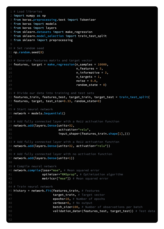
Developing a regression model
If you want to train regressions, you should do so.
The following instructions will show you how to create a feedforward neural network with a single output unit and no activation function using Keras:
As an alternative to class probabilities, neural networks are capable of predicting continuous values. Using our binary classifier (snippet 20.3) a single unit output layer was combined with a sigmoid activation curve to calculate the probability of an observation being in class 1. It is important to note that the sigmoid activation function constrained the output value to be between 0 and 1. Our output can be a continuous value if we remove that constraint by not having an activation function.
We should also use an appropriate loss function and evaluation metric, in our case the mean square error, since we are training a regression:
MSE=1n∑i=1n(yi^-yi)2where n is the number of observations; yi is the true value of the target we are trying to predict, y, for observation i; and ŷi is the model’s predicted value for yi.
Additionally, we did not have to standardize the features because we are using simulated data with scikit-learn, make_regression. However, standardization would be necessary in nearly all real-world cases.
Predicting the future
Making predictions using a neural network is what you want to do.
Using Keras, build a feedforward neural network, and then use predict to make predictions:

In Keras, it’s easy to make predictions. Our neural network can be trained using the predict method, which returns the predicted output for each observation once the features are passed as an argument. Using our solution, a neural network is set up to predict the probability of being classified as a class 1, so the predicted output is the probability of being classified as a class 1. The probability of an observation being class 1 is very high when its predicted value is very close to 1, while the probability of an observation being class 0 is very high when its predicted value is very close to 0. In our test feature matrix, the following is the predicted probability of the first observation being class 1:

array([ 0.83937484], dtype=float32)Visualize the history of training
When it comes to neural networks’ accuracy and loss scores, you want to find the “sweet spot.”
The following example shows how you can use Matplotlib to visualize the loss of the test set and training set over time:


The training and test accuracy can also be visualized using the same approach:
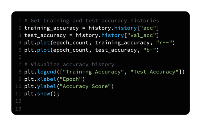

New neural networks perform poorly at first. Training data will lead to a decrease in the model’s error on both training and test sets as the neural network learns. At a certain point, the neural network begins “memorizing” the training data, leading to overfitting. A decrease in training error will result in an increase in test error once this starts happening. In many cases, there is a “sweet spot” at which the test error is at its lowest level (which is the error we are primarily interested in). When we visualize the training and test losses at each epoch in the solution, this effect is clearly visible. After epoch five, the training loss declines while the test loss increases, while the test error is lowest. Overfitting occurs at this point.
With weight regularization, overfitting can be reduced Regularization
A reduction in overfitting is what you want.
If you want to penalize the parameters of the network, also known as weight regularization, follow these steps:

In order to combat overfitting neural networks, parameters (i.e., weights) can be penalized so that they are driven to small values, creating a simpler model that is less prone to overfitting. Weight regularization or weight decay is the term used to describe this method. Weight regularization involves adding a penalty to the loss function, such as the L2 norm.
In Keras, we can include kernel_regularizer=regularizers.l2(0.01) in the layer’s parameters to add weight regularization. Using this example, 0.01 determines how much we penalize higher parameter values.
Using early stopping to reduce overfitting
A reduction in overfitting is what you want.
The following strategy is called early stopping and involves stopping training when the test loss stops decreasing:

As we discussed in snippet 20.7, In the first training epochs, both training and test errors will decrease, but as the network “memorizes” the data, the training error will continue to decrease even as the test error begins to rise. Consequently, monitoring the training process and stopping training when the test error increases is one of the most common and effective methods to counter overfitting. Early stopping is the name given to this strategy.
As a callback function in Keras, we can implement early stopping. During the training process, callbacks can be applied at various stages, such as at epoch ends. Specifically, we defined EarlyStopping(monitor=’val_loss’, patience=2) to monitor the test (validation) loss at every epoch and to interrupt training after two epochs if the test loss has not improved. Due to patience=2, we will instead get two epochs after the best model, which is not the best model. The ModelCheckpoint operation saves the model to a file after every checkpoint, allowing us to resume multiday training sessions if necessary. We would benefit from setting save_best_only=True, since it will only allow us to save the best models.
With dropouts, overfitting can be reduced
The goal is to reduce overfitting.
Make your network’s architecture noisy by using dropouts:

The dropout method is a powerful regularization method for neural networks. When a batch of observations is created for training, a proportion of the units in one or more classes are dropped out layers are multiplied by zero (i.e., dropped). Every batch is trained on the same network (i.e., the same parameters), but the network’s architecture differs slightly between batches.
Dropout works because it forces units to learn parameter values capable of performing under a wide variety of network architectures by continuously and randomly dropping units in each batch. That is, they learn to be robust to disruptions (i.e., noise) in the other hidden units, and this prevents the network from simply memorizing the training data.
Input and hidden layers can be dropped out. Dropping an input layer prevents its feature value from being introduced into the network for that batch. Input units can be dropped in portions of 0.2, and hidden units can be dropped in portions of 0.5.
Dropout can be implemented in Keras by adding Dropout layers to our network architecture. In each batch, a user-defined hyperparameter will be dropped from the previous layer. Keras assumes the input layer to be the first layer and does not add it using add. Dropout can therefore be added to the input layer by adding a dropout layer to the network architecture. Input_shape defines the shape of the observation data, as well as the proportion of the input layer’s units to drop 0.2. Following the hidden layers, a dropout layer with 0.5 is added.
Saving Model Training Progress
In case the training process is interrupted during the training of a neural network, you should save your progress.
You can save the model after every epoch by using the callback function ModelCheckpoint:

As soon as the test error stopped improving, we called the callback function ModelCheckpoint in conjunction with EarlyStopping. Another, more mundane reason for using ModelCheckpoint exists. Neural networks typically train for hours or days in the real world. There are many things that can go wrong during that time, including computers losing power, servers crashing, or inconsiderate graduate students closing your laptop.
Every epoch, ModelCheckpoint saves the model to alleviate this problem. The filepath parameter specifies the location where ModelCheckpoint saves the model after every epoch. A filename (e.g., models.hdf5) will be overwritten with the latest model every epoch if we include only the filename. In order to prevent overriding a file if the new model has a worse test loss than the previous one, we can set save_best_only=True and monitor=’val_loss’. The epoch number and test loss score can be included in the filename of every epoch’s model if we want to save it separately. Using the filepath model_[epoch:02d]_[val_loss:.2f].hdf5, the file containing the model saved after the 11th epoch with a test loss value of 0.33 would be model_10_0.35.hdf5 (note the epoch number is 0-indexed).