


Neural Networks and Neural Autoencoders as Dimensional Reduction Tools: Knime and Python
Neural Networks and Neural Autoencoders as Dimensional Reduction Tools: Knime and Python
Implemented with Knime and Tensor Flow in Python, analysing data in the middle of the diabolo.

In this section, I will follow a similar path, using a Neural Network with a Neural Autoencoder instead of the UMAP algorithm for dimension reduction. The work will be performed both in Knime, with Keras integration and in Python with TensorFlow. Once I've reduced the dimensions, I'll use DBSCAN to determine if the clusters created by the neural networks are identifiable. I'll share all code and workflows.
Neural Autoencoders
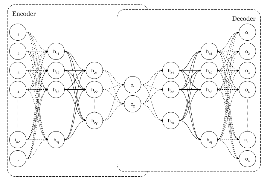
An example of a Simple Neural Autoencoder is shown in Fig. 1, where the input layer is the same size as the output, n, as per the image.
Using backpropagation to get an output equal to the input, autoencoders are trained as regular feedforward neural networks. As a result, they can reproduce the inputs that they were trained on. It is very likely that if we feed a trained network with inputs that are similar to those used during training, the output will be very close to the input. The input would not be considered usual or common if that didn't happen. Fraudulent credit card transactions are often detected using that capability. Since there are not many fraudulent card transaction data sets available, it makes sense to train the network on normal transaction data first, and if, at some point, the network cannot reproduce the input, we could declare fraud. Because of this, Autoencoders are considered unsupervised algorithms.
As you can see in Figure 1, there is a layer of minimum dimension in my original purpose of using autoencoders as a dimensional reduction technique. This is the centre of the diabolo.

As can be seen in the figure, n=2 is the dimension. Those layers are the codes. These are the latent spaces. The neural network will detect that we have various clusters of points based on the implicit classes in the input data at that point since we have codified the input. The neural network will display this in a two-dimensional graph in this case.
Structure and Sources
Using TensorFlow and Knime, we will perform this test.
There are some configurations you'll need in Knime to train a neural network with Keras.
This article is structured as follows:
Part 1. Dimensional reduction with Autoencoders
We will compare its implementation in Knime and Python step by step as we use simple dense autoencoders for dimensional reduction.
Part 2. Dimensional reduction with Dense Neural Networks
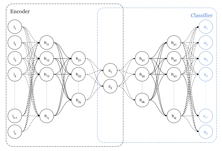
This will be followed by another interesting approach. We shall use an internal layer of 2 or 3 neurons within a dense neural network with an internal layer of 2 or 3 neurons, as the reference dataset for this test provides information about the class of each sample, rather than using an autoencoder. In Figure 3 we describe a network with a particular customised number of classes C=10, which corresponds to our dataset.
Similarly, we will analyse this implementation in Knime and Python step by step.
Knime workflows
Two different approaches are provided by Knime Workflow:
Part 1. Dimensional reduction with Autoencoders. The workflow will diverge in two different endings for 2D and 3D latent spaces. Alternatively,
Part 2. Dimensional reduction with Dense Neural Networks has also two different branches for 2D and 3D minimum dimension representation.
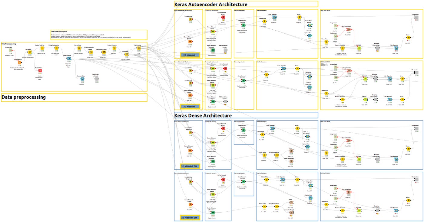
To help you understand the different branches, let me show you an overview of the entire workflow.
In Figure 3bis, yellow workflows correspond to autoencoder architecture in Part 1 for 2D and 3D and blue workflows correspond to dense architecture in Part 2.
Python codes
Two Python codes are available:
In KNIME_Replication_3D_Midpoint.py, the autoencoder method is used for training and inference, while KNIME_Replication_3D_Midpoint_DM.py utilizes a densely connected network for training and inference. Both codes assume a 3D latent space when executed without arguments. However, you can also pass an argument that indicates the desired latent space size, such as 3.
pyhton3 KNIME_Replication_3DMidpoint_DM.py 3Paid subscribers also have access to an auxiliary Python file, ml_functions.py, which defines and uses the class ModelGr and its methods in code.
Part 1. Dimensional reduction with Autoencoders
Data Preprocessing
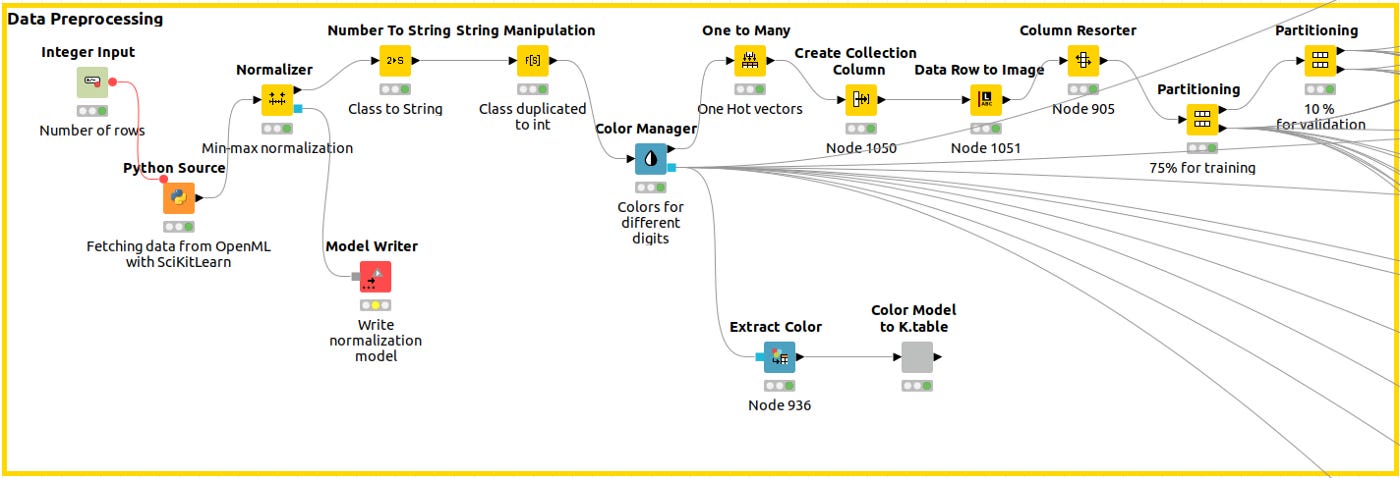
The Python Source Node captures the data, we normalize the data, and then, using the Color Manager node, we assign a unique color code to the class across the workflow so that every plot shows the same legend. A training partition and a validation partition are built next.
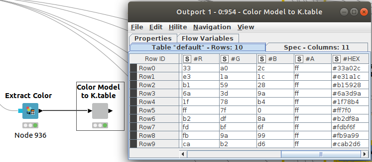
We can extract our color codes (in column #HEX) from previous nodes in Figure 5 so we can reuse them in Python. We can then compare the results more easily.
The first part of the Python code, which deals with fetching the data and partitioning it, can be found in Code 1.
# Dataset download
STORE_PATH = f"/home/isra/PycharmProjects/CodingTensorFlowV2/StoredResults/KNIME/3D_Midpoint_DM/{dt.datetime.now().strftime('%d%m%Y%H%M')}"
mnist = fetch_openml('mnist_784', version=1, as_frame=True)
df_data = mnist.data.iloc[:]
df_data = df_data.assign(digit_class=mnist.target.iloc[:].astype(int))
np_data = df_data.to_numpy()
np_data_images = np_data[:, 0:784]
np_data_images = np.reshape(np_data_images, (70000, 28, 28))
np_data_labels = np_data[:, 784]
#Partitioning, Test, Train, Validation
x_train,x_validation, y_train, y_validation = train_test_split(np_data_images,
np_data_labels, test_size=0.25,
random_state=42)
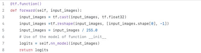
x_train,x_test, y_train, y_test = train_test_split(x_train, y_train,test_size=0.20, random_state=42)The forward method defined for the class ModelGr() performs normalization whenever forward inferences are performed. Look at lines 5 and 6 in code2.
Keras Neural Network Architecture
In Knime, neural architectures are represented by nodes that compose Keras Dense Layers. The figure below illustrates the definition in its global context.


The figure 7 shows a node that is special. It is a component that encapsulates several nodes and provides a configuration interface with functional parameters that determine the performance of its inner nodes. The sequence of layers is shown in figure 8, and the parameters of the component are shown in figure 9. The inner node definition will be entered by pressing CTRL+double clicking the Network Definition component as shown in Figure 8. A configuration window will open when you double click the network definition component. Here you can define layer sizes and activation functions.
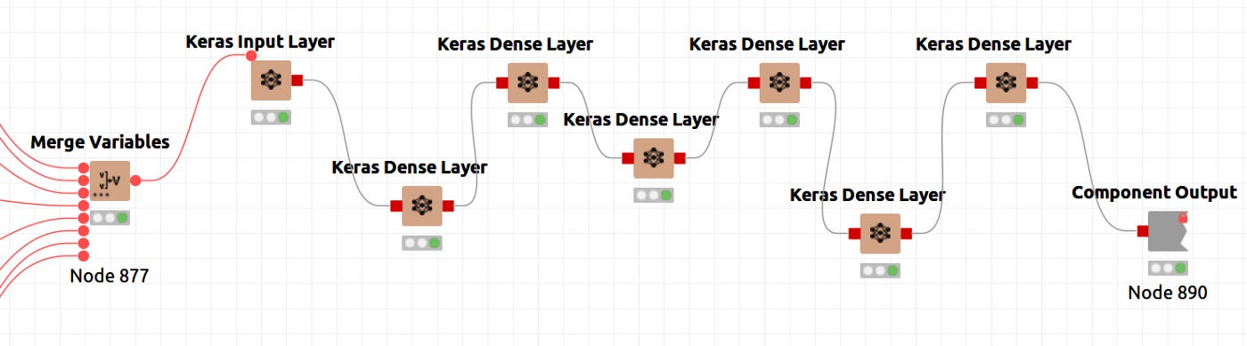

The input layer, five internal layers, and the output layer have been defined. As shown in Figure 9, the activation function is common to all layers, Hyperbolic Tangent. Beyond the parameters already mentioned, layer configuration parameters can be set up in each node's configuration, namely, the kernel and bias initializers, regularizers and constraints. The size is defined as 2 in the fourth layer of Figure 9 for the case of a 2D latent space. This alternative workflow is for 3D latent spaces.
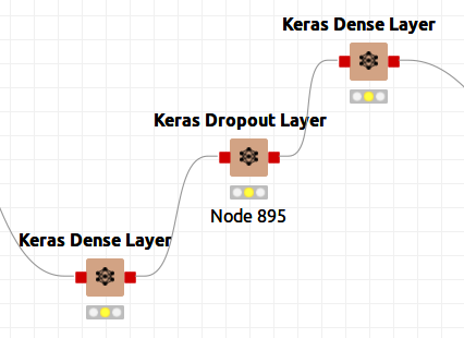
Figure 9bis shows that I could have used dropout layers to prevent overfitting even though I did not do so. Simply reconnect the nodes and add the dropout layer.
Python has defined a class ModelGr() that will be informed of the activation functions, layer sizes, and a number of layers when it is called. The model is defined as follows:
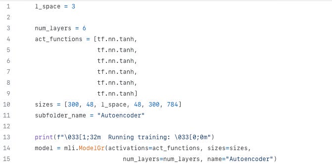
We define a sequential network (Line 15 of Code 4) and add recursively layers with size and activation functions included in the call (Lines 17+ of Code 4)
class ModelGr(object):
    # Dentro de la clase, se define la función __init__ que sirve en el momento de la instanciación.
    def __init__(self, activations, sizes, num_layers=6, name=None):

        assert len(activations) >= num_layers-1
        assert len(activations) <= num_layers
        assert len(sizes) == num_layers

        # Atención no se define el tamaño de la capa de recepción.
        # No estamos definiendo las matrices de transición sino las capas.

        self.num_layers = num_layers
        self.hidden_size = sizes

        self.nn_model = tf.keras.Sequential(name=f'sequential_{name}')

        for i in range(num_layers-1):
            self.nn_model.add(tf.keras.layers.Dense(units=sizes[i], activation=activations[i], name=f'Layer{i + 1}_{name}'))
            # Range solo va hasta el n-1. Es decir, no se crea la última capa
            # Entregamos los logits y ya hacemos como en el ejemplo anterior el softmax y la entropía

        if len(activations) < num_layers:
            self.nn_model.add(tf.keras.layers.Dense(units=sizes[num_layers-1], name=f'Model_{name}_Out_Layer'))
        elif len(activations) == num_layers:
            self.nn_model.add(tf.keras.layers.Dense(units=sizes[num_layers-1], activation=activations[num_layers-1], name=f'Layer{num_layers}_{name}'))
As can be seen in different Figures and codes, the networks have the following layers and sizes:
[784 (input), 300, 48, 2 or 3 (latent space), 48, 300, 784] and
the activation functions is hyperbolic tangent.
Training the network
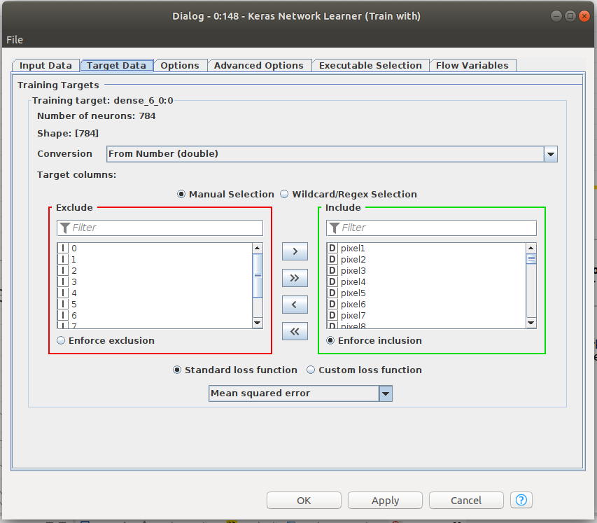
Knime makes it easy to train the network. Figure 6 shows that the Keras Network learner only needs training and validation data to function. Input data and target data for training need to be defined. To train an autoencoder, we need the same size input and target data, namely, the 784 pixels of the images from MNIST. A number of parameters are defined in that node, including the loss function that should be minimized in training. Please note that we have chosen MSE as our loss function. The input and the output vectors will be trained with the aim of minimizing the MSE since, ideally, they should be equal.
There is a training function in Python and TensorFlow. The RMSE, or Root Mean Square Error, is defined in Line 21 of Code 5, just as it is in Knime. ModelGr() defines the RMSE_loss() method in Code 5bis.
def run_training_enc(model_inst: mli.ModelGr, sub_folder: str, iterations: int = 2500,
                 batch_size: int = 32, log_freq: int = 200,
                 lim_loss: float = 0.05, graph_name: str = None):

    # Directorio para almacenar datos
    train_writer = tf.summary.create_file_writer(STORE_PATH + "/" + sub_folder)
    # Guardamos el grafo
    model_inst.plot_computational_graph(train_writer, x_train[:batch_size, :, :], graph_name)
    # Selección del optimizador
    optimizer = tf.keras.optimizers.Adam(learning_rate=0.001, beta_1=0.9, beta_2=0.999, epsilon=1e-08, amsgrad=False)  # Puede tener un argumento de learning rate
    # Vamos a la iteración de entrenamiento
    acc = 0
    for j in range(iterations):
        # Tomamos un batch
        image_batch, label_batch = mli.get_batch(x_train, y_train, batch_size)
        # image_batch = tf.Variable(image_batch) (Está en el libro pero no funciona)
        label_batch = tf.cast(tf.Variable(label_batch), tf.int32)
        # Calculamos los logits y la perdida
        with tf.GradientTape() as tape:
            logits = model_inst.forward(image_batch)
            loss = model_inst.RMSE_loss(logits, image_batch)
        gradients = tape.gradient(loss, model_inst.nn_model.trainable_variables)
        optimizer.apply_gradients(zip(gradients, model_inst.nn_model.trainable_variables))
        # Zona de Logs
        if j % log_freq == 0:
            max_idxs = tf.argmax(logits, axis=1)
            # El resultado de lo anterior e un tensor... Por eso necesitamos hacer un numpy()
            #acc = np.sum(max_idxs.numpy() == label_batch.numpy()) / len(label_batch.numpy())
            print(f"Iter: {j}, loss={loss:.3f}, (Scenario {graph_name})")
            with train_writer.as_default():
                tf.summary.scalar('loss', loss, step=j)
                #tf.summary.scalar('accuracy', acc, step=j)
                # log the gradients
            model_inst.log_gradients(gradients, train_writer, j)
        if loss <= lim_loss:
            print(f'\033[1;31m \nEnd for limit Loss={loss:.3f} \033[0;0m')
            break
Training functions for autoencoders
# Función de pérdidas RMSE
@staticmethod
def RMSE_loss(ypred, ylabel):
ylabel = tf.cast(ylabel, tf.float32)
ylabel = tf.reshape(ylabel, [ylabel.shape[0], -1])
ylabel = ylabel / 255.0
#loss = tf.reduce_mean(tf.square(ypred - ylabel))
mse = tf.keras.losses.MeanSquaredError()
loss = mse(ypred, ylabel)
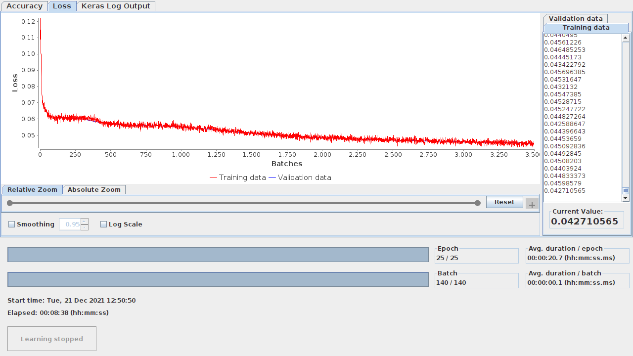
return lossAs for checking how the training evolved, you can do that in both approaches. Knime allows you to view the learning monitor by right clicking on the Keras Network Learner node. Figure 10.1 illustrates the learning monitor.
TensorBoard is a tool for analyzing TensorFlow networks.
TensorBoard provides the visualization and tooling needed for machine learning experimentation:
-Tracking and visualizing metrics such as loss and accuracy
-Visualizing the model graph (ops and layers)
-Viewing histograms of weights, biases, or other tensors as they change over time
-Projecting embeddings to a lower dimensional space…
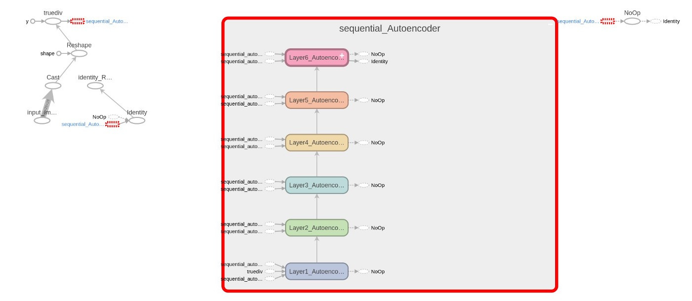
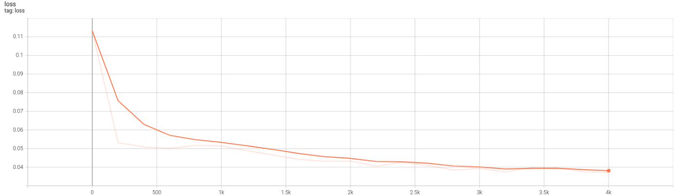
Several new lines of code are added to Code 5 (6,22,23,30+) to collect data on training and network graphs, weights, and losses. TensorBoard is launched automatically by the shared Python codes, both dense and autoencoder. Figures 10.2 and 10.3 show the graph and the evolution of losses.
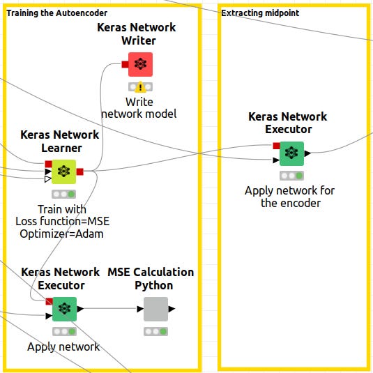
Extracting the midpoint
It is now time to get the output of the networks, which have been configured as Neural Autoencoders. Note that in Knime, there is a red output port for the Keras Network Learner. Those outputs are the model-trained networks. The network is then executed by connecting a node informed with the model and data to the Keras Network Executor. Caution is advised.
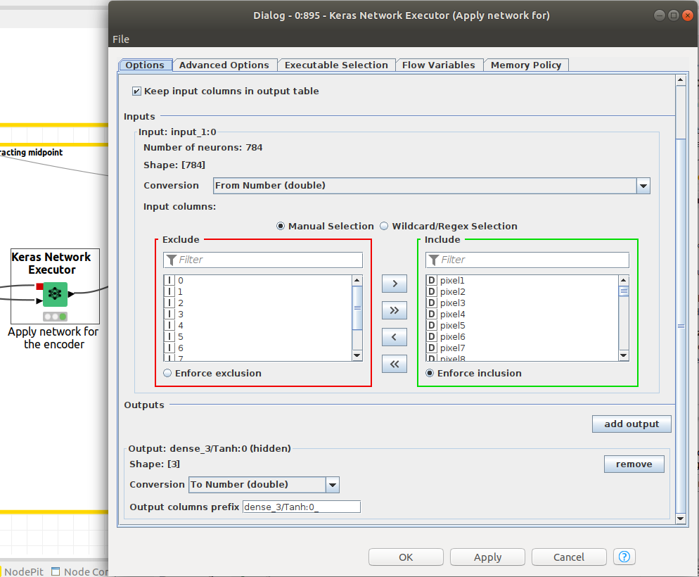
We need the Keras network execution node to deliver that paticular output since we want to extract the latent space from the autoencoder. This is done by defining the output layer as the layer that corresponds to the latent space. In Figure 12, the Network Executor node is configured to output the latent space.
To extract the midpoint from a sequential network, we had built a Python class called Encoder(). The __init__ method, when used to enumerate an object as encoder(), will add the layers of the network from the initial layers to the minimum sized layer, that is, the latent space, once the object is defined as encoder(). Code 6, Line 9 describes this condition.
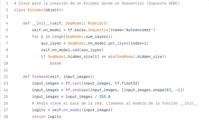
A forward method is defined for inferring the Encoder. It is shown in Code 7.
 def forward(self, input_images):
        input_images = tf.cast(input_images, tf.float32)
        input_images = tf.reshape(input_images, [input_images.shape[0], -1])
        input_images = input_images / 255.0
        # Ahora viene el paso de la red. Llamamos al modelo de la función __init__
        logits = self.nn_model(input_images)
        return logits
Encoder has been defined as the portion of the neural network from the initial layer to the minimum sized layer so the forward method will deliver the latent space.
Results for autoencoders networks
Graphical results for latent space will be shown.
2D Results and attempt to get clusters.
In Figure 12 and 13, the 2D latent space of the autoencoder is plotted for both environments, Knime and Python. It can be checked that some sort of order and coherence can be perceived by human eye but, applying DBSCAN algorithm on that data won’t lead to any cluster related to those that were defined in the latent space of the autoencoder.