

Optimizing Financial Analysis: A Deep Dive into Machine Learning and Neural Networks in Options Pricing
Exploring the Integration of Advanced Computational Techniques for Enhanced Market Predictions and Risk Assessment

computational techniques has become a cornerstone for both academic research and practical applications. The utilization of machine learning, particularly neural networks, offers a robust framework for delving into market dynamics and improving predictive accuracies. This paper explores the integration of advanced machine learning algorithms with traditional financial models like Black-Scholes to enhance the precision of options pricing and risk management strategies.
There is no source code for this article. All code is in the article itself.
Recent advancements in computational power and the availability of high-frequency trading data have enabled the deployment of more complex models that can learn from vast datasets and uncover patterns that were previously unidentifiable. Neural networks, with their deep learning capabilities, are at the forefront of this revolution, providing the flexibility and scalability required to model the nonlinear complexities of financial markets. By blending these computational techniques with established financial theories, this paper aims to bridge the gap between traditional models and modern requirements, offering insights that are critical for developing more resilient and efficient financial systems.
!pip3 install --upgrade tensorflow-gpu
import tensorflow as tf
tf.test.gpu_device_name()
Initially, the code utilizes the pip package manager to elevate the TensorFlow-GPU library to its most recent version. Subsequently, it proceeds to import the TensorFlow library. Following this, it calls upon the test.gpu_device_name() function within TensorFlow to ascertain the availability of a GPU device for computational purposes.
This script serves the purpose of updating the TensorFlow GPU library to the latest version and determining the usage of GPU for computational tasks within TensorFlow. Leveraging GPU support in TensorFlow can notably hasten the process of training machine learning models especially when handling extensive datasets and intricate neural network structures. By harnessing the GPU for computations, TensorFlow can exploit the parallel processing capabilities offered by the GPU, thereby accelerating training durations in contrast to sole reliance on the CPU.
import warnings; warnings.simplefilter('ignore')
import datetime as dt
import numpy as np
import matplotlib.pyplot as plt
import matplotlib.mlab as mlab
import pandas as pd
This piece of code imports the required modules and establishes a basic warning filter to disregard any warnings throughout the code’s operation.
Each segment of the code serves a distinct purpose:
- By bringing in ‘warnings’: it enables the handling of warnings through the warnings module.
- ‘warnings.simplefilter(‘ignore’)’: arranges a rudimentary warning filter to dismiss all warnings that arise while the code runs. This feature proves handy when you prefer not to view warnings on the console or disrupt the program’s outcome.
- ‘import datetime as dt’: introduces the datetime module as ‘dt’, facilitating work with dates and times in Python.
- ‘import numpy as np’: accesses the NumPy library as ‘np’, a robust tool for numerical operations in Python.
- ‘import matplotlib.pyplot as plt’: pulls in the pyplot module from the Matplotlib library as ‘plt’. Matplotlib serves as a visualization tool for generating plots in Python.
- ‘import matplotlib.mlab as mlab’: brings in the mlab module from Matplotlib, which incorporates a set of functions that have become outdated and relocated within Matplotlib.
- ‘import pandas as pd’: adds the pandas library as ‘pd’, offering substantial capabilities for data manipulation and analysis in Python.
Employing this code empowers you to engage with dates, conduct numerical computations, plot data, and handle information effectively without any disruption caused by warnings. It prepares the groundwork with essential resources and configurations for seamless execution of subsequent code.
import io
DF = pd.read_csv('/content/drive/MyDrive/Centrale Supelec/DeepLearningFinance/TD8/TP8_ES_options.csv.gz',compression='gzip',index_col=0)
DF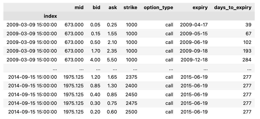
The following script imports data from a designated CSV file and allocates it to a pandas DataFrame labeled DF. The file is compressed using gzip, specified by defining the compression parameter as ‘gzip’. By setting index_col=0, the initial column of the CSV file becomes the DataFrame’s index.
This piece of code is vital for swiftly loading a compressed CSV file into a DataFrame in Python. Decompression occurs in real-time during loading, resulting in saved disk space and accelerated data processing. This code is frequently utilized for managing substantial datasets saved in compressed file types.
DF['mid_option'] = (DF.ask + DF.bid)/2 ; ## Mid Price de l'option
DF['spread'] = (DF.ask - DF.bid)/DF.mid ; ## Spread # Spread de l'option normalisé par S0
DF['Price_rescale'] = DF.mid_option/DF.mid ; ## Mid Price rescale
DF['Strike_rescale'] = DF.strike/DF.mid ## Strike rescale
DF['Time2Mat_year'] = DF.days_to_expiry/365 ## Maturité en Années
Within this code excerpt, a range of computations and data modifications are being executed utilizing columns sourced from a DataFrame named DF. Let’s delve into the purpose behind each operation:
Determining the mid price of an option through the calculation of the average between ask and bid prices is referred to as mid_option.
The spread operation finds the disparity of the option by dividing the variance between the ask and bid prices by the mid price. This adjustment ensures the spread is proportional to the underlying asset price.
Price_rescale involves adjusting the mid option price by dividing it by the mid price, facilitating a comparative analysis of the option price to the underlying asset price.
Scaling down the strike price of the option through Strike_rescale by dividing it by the mid price eases the comparison of the strike price concerning the underlying asset price.
Time2Mat_year lets you transform the option’s expiry days into years by dividing them by 365.
These calculations are prevalent in the financial sector, specifically within options pricing and risk management. Standardizing prices concerning the underlying asset price and converting time units serve as fundamental techniques to simplify comparisons and computations. This code snippet plays a pivotal role in preparing and refining the data for subsequent analysis or modeling within the financial realm.
Calls = DF[DF["option_type"] == "call"]
Puts = DF[DF["option_type"] == "put"]
The snippet of code you’re examining serves to sift through a DataFrame labeled DF, segmenting it into two distinct entities, Calls and Puts. This segmentation is achieved by cherry-picking rows from DF where the “option_type” field holds the value “call” for Calls and “put” for Puts.
This coding technique proves invaluable when tackling extensive data collections, allowing for a systematic segregation of information hinged on predetermined conditions. Here, it facilitates the bifurcation of data grounded on the “option_type” attributes, thereby simplifying the execution of tailored procedures on call and put data autonomously. These operations can span diverse activities like computations, assessments, or visual representations.
log_ret_calls = np.log(pd.DataFrame(Calls['mid'].groupby('index').first())).diff()
Calls["logret"] =  log_ret_calls
Calls.dropna(inplace=True)
Calls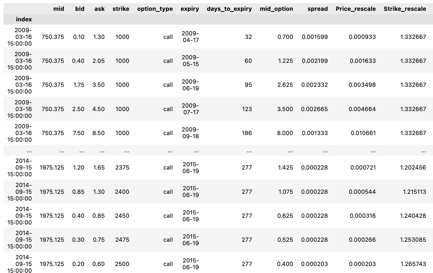
This particular script facilitates the computation of logarithmic returns within distinct groups of data labeled “Calls,” encapsulating stock details.
To streamline the process, here’s a rundown of the series of actions:
1. Employing the function: log_ret_calls = np.log(pd.DataFrame(Calls[‘mid’].groupby(‘index’).first())).diff(). This operation entails deriving the natural logarithm of the primary value within each cluster of the “mid” column in the “Calls” dataset and subsequently evaluating the variance between successive entries.
2. Integration of a new element: Calls[“logret”] = log_ret_calls. By executing this segment, a fresh segment labeled “logret” is appended to the “Calls” data structure, housing the computed logarithmic returns.
3. Data refinement: Calls.dropna(inplace=True). This directive clears out any incomplete entries (NaN) that arise from the logarithmic return calculation, thereby ensuring data consistency.
4. Last but not least, the script generates the adapted “Calls” dataset, inclusive of the lately integrated “logret” column.
In financial contexts, logarithmic returns surface prominently for gauging investment efficacy. Their preference stems from their cumulative nature over time and additional statistical attributes conducive to modeling and assessment purposes.
log_ret_puts = np.log(pd.DataFrame(Puts['mid'].groupby('index').first())).diff()
Puts["logret"] =  log_ret_puts
Puts.dropna(inplace=True)
Puts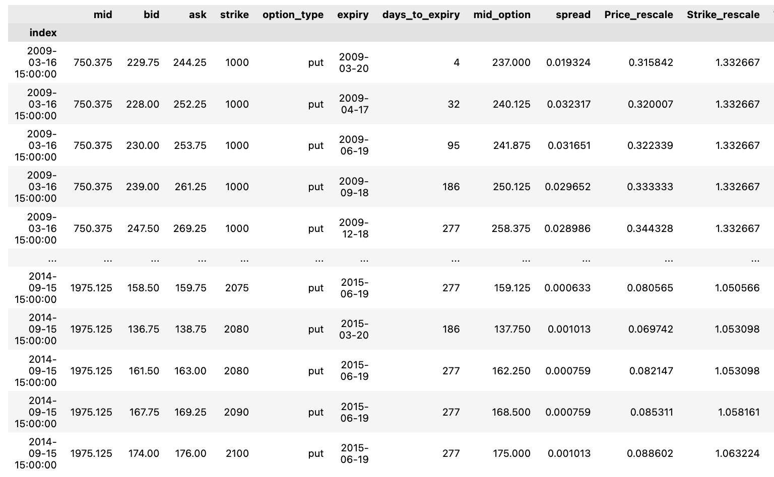
This particular code snippet deals with financial information, likely focusing on options data, and employs the pandas library in Python. Below is a breakdown of its functionality:
To start, it computes the logarithmic returns for the options data. This involves extracting the mid price from the puts option data, applying the np.log function to derive the logarithm of these mid prices, grouping the data by index, selecting the initial data entry within each group, and subsequently determining the variance between consecutive values with the diff function. Consequently, this process generates the logarithmic returns for the puts options data.
Next, the code adds the calculated log returns to a new column. It constructs a fresh column titled “logret” within the Puts DataFrame and populates it with the computed logarithmic returns.
Subsequently, it eliminates any rows containing empty values. By utilizing the dropna function with the parameter inplace=True, the code eradicates rows in the Puts DataFrame that exhibit missing values across any column.
Lastly, it returns the updated DataFrame. Upon executing the aforementioned tasks, the code yields the revised Puts DataFrame, which now showcases the log returns for the put options data sans any absent values.
In financial scrutiny, leveraging logarithmic returns stands as a prevalent practice to standardize the data, facilitating its analysis and comparison across different financial instruments over time. Additionally, the code filters out any rows containing missing values to uphold the quality and reliability of the data employed for subsequent analysis or modeling purposes.
Calls['vol_roll7d'] =  log_ret_calls.rolling(7).std();
Calls['vol_roll14d'] = log_ret_calls.rolling(14).std();
Calls['vol_roll49d'] = log_ret_calls.rolling(49).std();
Calls.dropna(inplace=True)


Puts['vol_roll7d']  = log_ret_puts.rolling(7).std();
Puts['vol_roll14d'] = log_ret_puts.rolling(14).std();
Puts['vol_roll49d'] = log_ret_puts.rolling(49).std();
Puts.dropna(inplace=True)
This script is designed to compute the rolling standard deviation of log returns for call (options to buy) and put (options to sell) datasets.
It appends new columns in the ‘Calls’ and ‘Puts’ DataFrames, storing the rolling standard deviation values calculated across varying windows of 7, 14, and 49 days.
By leveraging the rolling() function, it computes rolling statistics, specifically standard deviation, using custom window sizes to smooth out the data and unveil underlying trends or volatility patterns.
Following the computation, it eliminates any rows containing missing values (NaN) from the DataFrames using the dropna() method with inplace=True.
In essence, this code aids in scrutinizing the options market’s volatility by analyzing the rolling standard deviation of log returns for both calls and puts. This enhances the data’s readiness for further scrutiny and interpretation.
Calls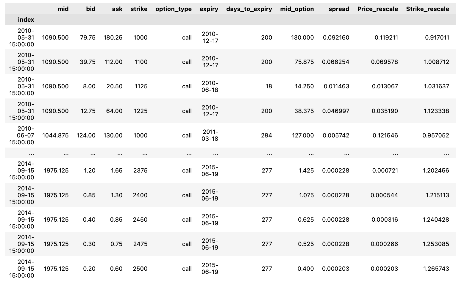
Let’s see all of the call options.
Puts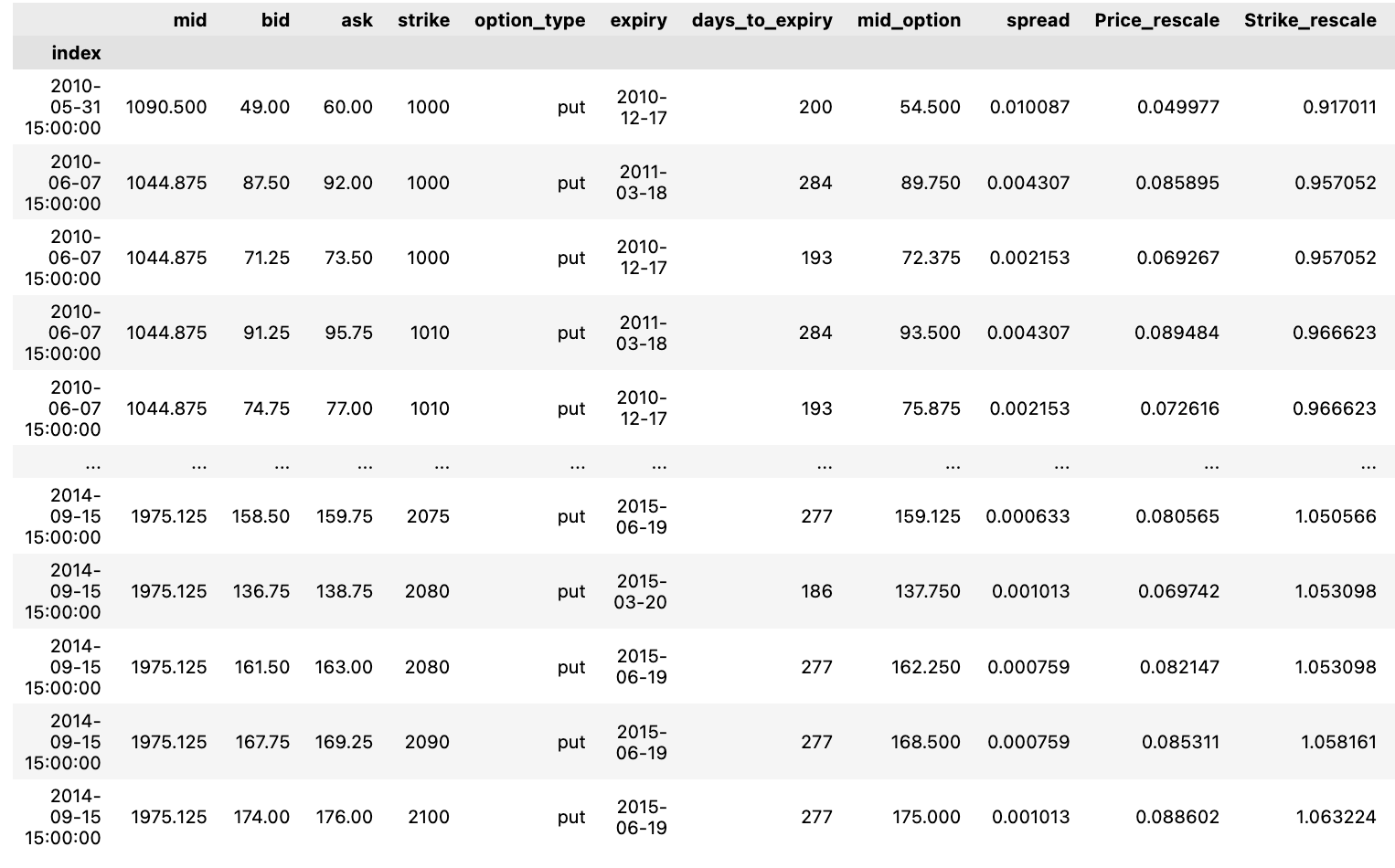
Let’s see the all of the put options.
Exploring theoretical pricing calculations under the Black-Scholes model.
Option_Strikes = np.unique(DF.strike)
Option_Maturity = np.unique(DF.days_to_expiry)
The following snippet of code captures distinct values from the “strike” column in the DataFrame labeled as “DF” and saves them into the variable named “Option_Strikes.” Similarly, it records unique values from the “days_to_expiry” column in the DataFrame as “Option_Maturity.”
This code proves valuable for isolating distinct strike prices and maturities within the DataFrame. Such information serves as a solid foundation for any subsequent analysis or computations, particularly within the realm of options trading or any other scenario necessitating thorough data assessment. By detecting singular values in these specific columns without redundancy, this methodology becomes pivotal for shaping well-informed decisions grounded in the dataset at hand.
Examination of Insufficient Parameters:
Now, let’s explore the process of choosing predictors:
- Spread normalized by the mid-price
- Time remaining until maturity.
Our dataset will be divided into training and testing subsets. Specifically, 80% of the data will be designated for training, with the remaining 20% set aside for testing.
Within the 80% training data, a 20% portion will be used for cross-validation.
To prevent overfitting, an early stopping mechanism will be implemented to stop the training process before the loss increases again in the cross-validated subset.
from sklearn.metrics import mean_squared_error, mean_absolute_errorIn this script, two essential functions — mean_squared_error and mean_absolute_error — are being imported from the sklearn.metrics module. These functions play a crucial role in assessing the precision of predictions made by a machine learning model.
The mean_squared_error function computes the average of the squared variances between predicted and actual values, offering insight into the proximity of predictions to actual results. A lower mean squared error signifies a closer alignment between predicted and actual values, indicating a stronger model fit.
On the other hand, the mean_absolute_error function determines the average of absolute variances between predicted and actual values. Notably, this metric is less influenced by outliers when compared to mean squared error. Similar to mean squared error, a reduced mean absolute error implies a more accurate model fit with the dataset.
These functions are commonly utilized in regression scenarios to gauge the effectiveness of predictive models. Through the inclusion of these functions, the process of evaluating predictive model performance is streamlined, eliminating the need to develop these metrics from the ground up.
from keras.models import Sequential
from keras.layers import Dense , Dropout  ,LeakyReLU
from keras.optimizers import Adam
from sklearn.model_selection import train_test_split

X_train, X_test, Y_train, Y_test = train_test_split(Calls, Calls[['mid_option']], test_size=0.1, shuffle=True)#'Price_rescale''mid_option'
The code starts off by importing essential classes and functions from the keras library needed to construct and train neural network models, like Sequential, Dense, Dropout, LeakyReLU, and the Adam optimizer. Additionally, it brings in the train_test_split function from scikit-learn, which is utilized to divide the data into training and testing sets.
Following that, the data undergoes splitting into training and testing sets through the deployment of the train_test_split function. Specifically, within the ‘Calls’ dataset, the ‘mid_option’ column serves as the target variable, segregating the data into X_train (training features), X_test (testing features), Y_train (training target values), and Y_test (testing target values).
The code sets the test_size parameter to 0.1, designating 10% of the data for testing purposes, while the remaining 90% is allocated to training. Enabling shuffle=True guarantees randomizing the data before dividing it, a measure undertaken to avert any potential bias during the split.
By partitioning the data into training and testing sets, the neural network model can be trained on the training data and then assessed on unseen test data. This standard procedure in machine learning serves the purpose of evaluating the model’s capacity for generalization and mitigating overfitting issues.
X_train = X_train[['Strike_rescale','days_to_expiry']]
X_test  = X_test[['Strike_rescale','days_to_expiry']]
In this script, the ‘Strike_rescale’ and ‘days_to_expiry’ columns are being extracted from the training set X_train and the test set X_test, respectively. Through the use of double square brackets enclosing the column names, this extraction process is executed.
This snippet serves to sift through the data and retain solely the essential columns needed for subsequent operations like model training, prediction generation, or data analysis. The act of singling out particular columns enables a concentrated analysis on pertinent features crucial for the intended task, effectively shrinking the data’s complexity and boosting computational performance.
def Dense_ANN(activ_func = 'relu',X_train_shape = X_train.shape[1]):

  activ_fn = activ_func
  model = Sequential()
  model.add(Dense(200 , activation = activ_fn ,input_dim = X_train_shape))
  model.add(Dense(150,activation= activ_fn))
  model.add(Dense(100,activation= activ_fn))
  model.add(Dense(80,activation= activ_fn))
  model.add(Dense(50,activation= activ_fn))
  model.add(Dense(30,activation= activ_fn))
  model.add(Dense(20,activation= activ_fn))
  model.add(Dense(10,activation= activ_fn))
  model.add(Dense(5,activation= activ_fn))
  model.add(Dense(1,activation= activ_fn))
  Opt_Adam = Adam(learning_rate = 1e-3) ## On reduit le learning rate par default car difficulté a converger au debut
  model.compile(loss = 'mse' , optimizer = Opt_Adam , metrics=["mse"])
  return model
This particular function is designed to set up a complex artificial neural network (ANN) consisting of numerous dense layers. Within the function, there are two optional parameters. The first one, activ_func, allows the selection of the activation function to be applied across all layers. The second one, X_train_shape, is responsible for defining the shape of the input data X_train.
To kick things off, the function starts by creating a Sequential model, which essentially presents a simple linear arrangement of layers. Subsequently, multiple Dense layers are incorporated into the model, featuring a reduction in the number of nodes as each layer unfolds. These Dense layers essentially symbolize fully connected segments within the neural network. Notably, the nodes in these layers are set at varying quantities: 200, 150, 100, 80, 50, 30, 20, 10, 5, and 1 consecutively.
The activation function in all layers is dictated by the activ_func parameter that is fed into the function. By default, the Rectified Linear Unit (ReLU) activation function steps in.
Once the layers are structured, the model undergoes a compilation phase. During this process, the Mean Squared Error (MSE) is designated as the loss function, and the optimizer chosen is Adam, sporting a specific learning rate of 1e-3.
This piece of code comes in handy particularly when constructing neural networks for regression purposes. It streamlines the task of setting up a deep ANN framework that offers flexibility with its activation function and input shape. Simultaneously, it primes the model for both training and assessment. Essentially, it simplifies the complex process of constructing and compiling the neural network’s architecture to facilitate seamless and swift experimentation with diverse setups.
ANN = Dense_ANN(activ_func = 'relu',X_train_shape = X_train.shape[1])
callback = tf.keras.callbacks.EarlyStopping(monitor='val_loss', patience=20,mode='auto', baseline=None,
                                            restore_best_weights=True)
ANN.fit(X_train,Y_train,validation_split=0.2,epochs=1000, callbacks=[callback])
The provided code snippet demonstrates the creation and training of an artificial neural network (ANN) through TensorFlow’s Keras API. It outlines the neural network’s structure as a dense network with ReLU activation function.
To enhance training efficiency and prevent overfitting, the code incorporates tf.keras.callbacks.EarlyStopping. This callback interrupts the training process if the monitored quantity, in this case ‘val_loss’, ceases to improve after 20 epochs. Consequently, the model is fit on X_train and Y_train data sets, with 20% designated for validation through the validation_split parameter.
The training regimen extends to a maximum of 1000 epochs, yet the process will halt prematurely if the validation loss fails to enhance over 20 consecutive epochs, a feature governed by the EarlyStopping callback. This strategy not only averts overfitting but also conserves computational resources by curtailing redundant training iterations.
resultats = Y_test ; resultats["mid_predict"] = ANN.predict(X_test).flatten().tolist() ;
resultats["err"] = round((np.abs(resultats.mid_predict - resultats.mid_option)/resultats.mid_option)*100,2) ; resultats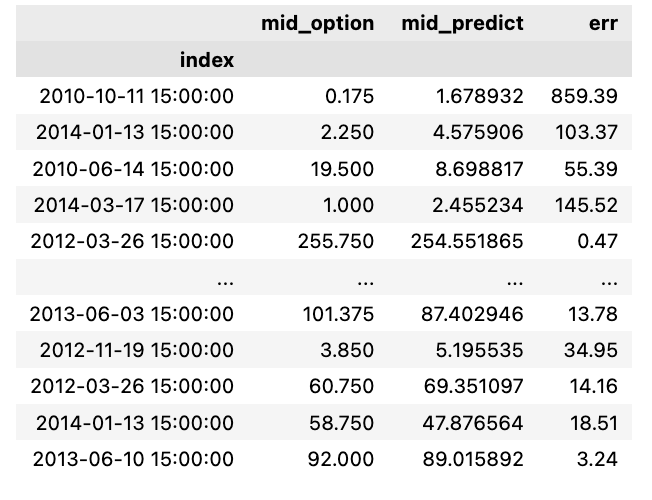
In this code snippet, the evaluation of a neural network model’s performance is carried out by cross-referencing its predictions with the actual values present in the test set.
Let’s delve into the breakdown of the code:
resultats = Y_test: This line involves assigning the test labels (Y_test) to a variable named resultats.
resultats[“mid_predict”] = ANN.predict(X_test).flatten().tolist(): Here, the neural network model (ANN) generates predictions for the test features (X_test); these predictions are then flattened into a 1D array and converted into a list. The resulting predictions are stored in the resultats DataFrame under the column labeled “mid_predict”.
resultats[“err”] = round((np.abs(resultats.mid_predict — resultats.mid_option)/resultats.mid_option)*100,2): This section of the code computes the error rate. It involves finding the absolute variance between the predicted values and the real values (mid_option), then dividing this variance by the actual values, multiplying it by 100 to get a percentage error, and rounding it off to two decimal places. The determined error rate is subsequently added to the resultats DataFrame under the column titled “err”.
Subsequently, the finalized resultats DataFrame, encompassing the test labels, predicted values, and error rates, is yielded as the output of the code snippet.
This code proves instrumental in assessing a neural network model’s performance by contrasting its predictions against the actual values within a testing dataset. Such an evaluation not only aids in gauging the model’s accuracy but also in pinpointing potential areas where it might be lagging. The error estimation further furnishes quantitative insights into the model’s efficiency, spotlighting the percentage variance from the authentic values. This analysis stands as a pivotal tool for machine learning experts, empowering them to draw informed conclusions regarding the model’s efficacy and avenues for enhancements.
We evaluate the relative prediction error for every price point, finding it more fitting to consider the relative error over the absolute discrepancy.
fig , ax = plt.subplots(2,1,figsize = (20,14))
ax[0].stem(np.arange(0,resultats.shape[0],1), resultats.mid_option.values, linefmt='grey', markerfmt='D', bottom=0.7, use_line_collection=True,label = "Price")
ax[0].stem(np.arange(0,resultats.shape[0],1), resultats.mid_predict.values, linefmt='grey', markerfmt='D', bottom=0.7, use_line_collection=True,label = "Price Predicted")
ax[0].set_ylabel("Options Prices")
ax[0].legend()
ax[0].set_title("Price Predicted vs Price")
ax[0].grid()
ax[1].stem(np.arange(0,resultats.shape[0],1), resultats.err.values, linefmt='red', markerfmt='D', bottom=0.7, use_line_collection=True)
ax[1].grid()
ax[1].set_ylabel("Erreur Relative")
ax[1].set_title("Erreur relative between Price Predicted and Prices")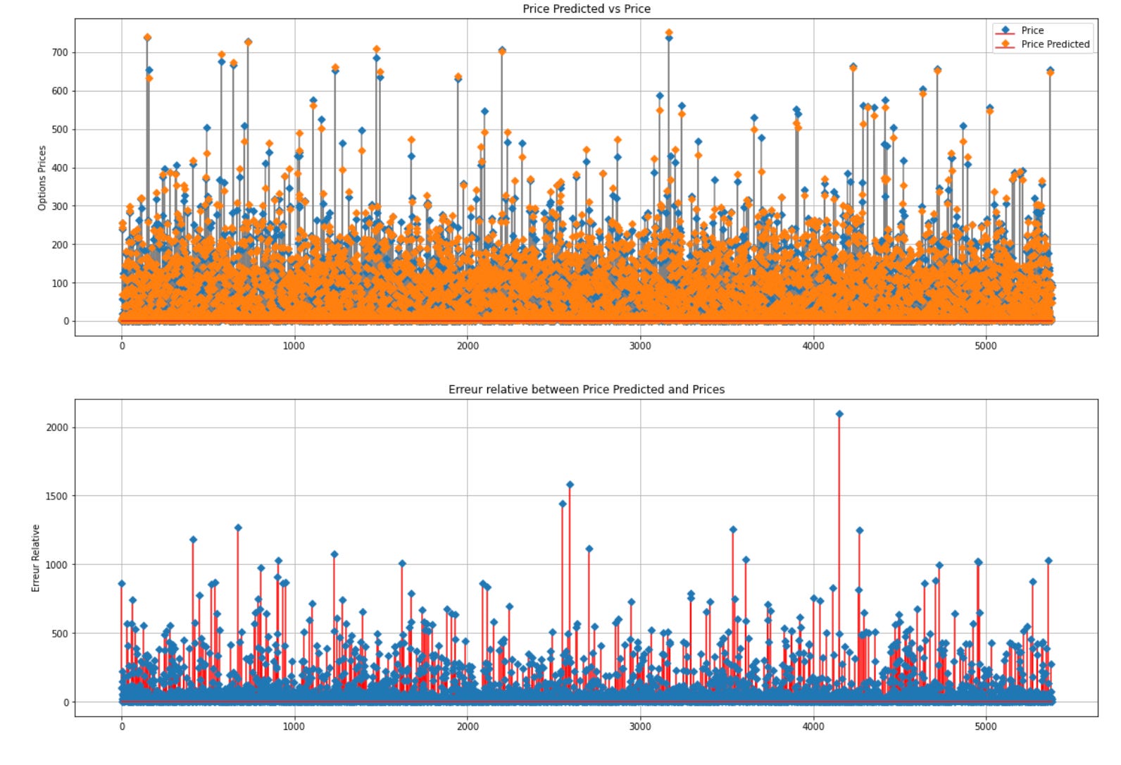
Above is the code snippet that generates a figure containing two vertically arranged subplots. The first subplot exhibits a stem plot that juxtaposes the genuine option prices (‘Price’) against the anticipated option prices (‘Price Predicted’). It designates ‘Option Prices’ as the y-label, incorporates a legend, entitles it ‘Price Predicted vs Price’, and toggles on the grid for enhanced clarity. The second subplot showcases a stem plot of the relative error (‘Relative Error’) between the predicted and actual prices. It assigns ‘Relative Error’ as the y-label, entitles it ‘Relative Error between Price Predicted and Prices’, and activates the grid for better visibility.
Employing matplotlib, the code graphically represents and contrasts the actual and predicted option prices alongside the relative errors. This visual aid facilitates the evaluation of price prediction accuracy and comprehension of relative errors, thereby contributing to model validation and assessment. The stem plot serves to align data points with the x-axis, enabling a lucid display of divergences between predicted and actual prices.
MSE_ANN1 = mean_squared_error(resultats.mid_option,resultats.mid_predict)
MAE_ANN1 = mean_absolute_error(resultats.mid_option,resultats.mid_predict)
print(f"La mean squared error est de : {MSE_ANN1}")
print(f"La mean absolute error est de : {MAE_ANN1}")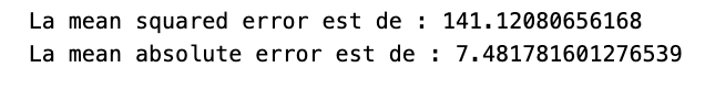
The following script computes the Mean Squared Error (MSE) and Mean Absolute Error (MAE) to gauge the disparities between a model’s predicted values and the actual outcomes.
MSE, determined by averaging the squares of the deviations between predicted and actual values, accentuates substantial errors by squaring the individual errors, hence being sensitive to outliers in the data.
On the other hand, MAE, obtained by averaging the absolute deviations between predicted and actual values, offers a more straightforward assessment of errors compared to MSE since it doesn’t involve squaring the errors.
MSE and MAE serve as prevalent yardsticks for assessing regression models’ efficacy, offering insights into how well the model conforms to the data by indicating the proximity of predicted values to actual outcomes.
Reviewing the MSE and MAE values allows us to evaluate the model’s performance and grasp the extent of deviation between its predictions and real-world values. These metrics are pivotal for contrasting various models, fine-tuning hyperparameters, and enhancing overall model performance.

