

Optimizing Portfolio Performance: A Guide to Effective Backtesting
Leveraging Python for Advanced Financial Analysis and Risk Management

In this comprehensive guide, we delve into the intricacies of backtesting and portfolio optimization using Python, a powerful tool in the realm of quantitative finance. The journey begins with the installation of essential Python packages, ensuring a robust foundation for complex financial analyses. We explore the loading and preparation of the Barra dataset, a cornerstone for risk prediction, and the implementation of various Python libraries like scipy, pandas, and matplotlib for data manipulation and visualization.
Key concepts such as Winsorization and factor exposures estimation are meticulously examined. The guide further outlines the construction of an optimized portfolio, integrating factors like specific variance, alpha factors, and transaction costs into the decision-making process. We then shift our focus to the practical aspects of building a trade list, managing optimal holdings, and attributing profit-and-loss. Finally, we provide a detailed exploration of portfolio characteristics, offering insights into long and short positions, net positions, and gross market values. This guide serves as a valuable resource for finance professionals and enthusiasts seeking to harness the power of Python in portfolio management and risk assessment.
Install packages
import sys
!{sys.executable} -m pip install -r requirements.txt
This python code is used to install the necessary packages or libraries required for a particular project. First, the sys library is imported, which allows access to system-specific parameters and functions. Then, the pip module is used to manage and install python packages. The command !{sys.executable} -m pip ensures that the correct version of pip is being used, and the install command is used to specify that we want to install the packages. The -r requirements.txt flag indicates that the packages listed in the requirements.txt file will be installed. This file typically includes a list of dependencies or packages that are needed for the project to run properly. By running this code, we can efficiently install all the required packages and dependencies without having to manually install each one.
import scipy
import patsy
import pickle

import numpy as np
import pandas as pd

import scipy.sparse
import matplotlib.pyplot as plt

from statistics import median
from scipy.stats import gaussian_kde
from statsmodels.formula.api import ols
from tqdm import tqdm
The code first imports various libraries such as scipy, patsy, pickle, numpy, pandas, scipy.sparse, matplotlib.pyplot, statistics, scipy.stats, and statsmodels.formula.api, as well as the tqdm library that allows for creating progress bars. These libraries provide various functions and methods that will be used in the code. Next, the code uses the import statement to access these libraries and make their functions available for use. For example, the from statistics import median statement imports the median function from the statistics library. Finally, the code uses the as keyword to create aliases for these libraries. This allows the developer to refer to these libraries using shorter, more convenient names. For example, instead of writing scipy.sparse.csr_matrix, the developer can simply use scipy.sparse.csr_matrix in their code. Overall, this code is used at the beginning of a Python code to import necessary libraries and make their functions and methods available for use.
Data Preparation: Loading Pre-Processed Barra Data for Risk Prediction
In this section, we’ll work with the Barra dataset, which is instrumental in predicting risk factors. Dealing with raw Barra data can be an intensive process, often leading to significant slowdowns in backtesting. Hence, it’s advantageous to handle pre-processed data. For ease of use, the Barra data has been pre-processed and stored in pickle files, which we’ll be using.
The following code demonstrates how to load the factor data for the year 2004 from a pre-processed file named pandas-frames.2004.pickle. Additionally, we’ll load covariance data for the years 2003 and 2004 from covariance.2003.pickle and covariance.2004.pickle respectively. It’s advisable to tailor the range of data according to your backtesting needs. A good starting point is to use two to three years of factor data.
Importantly, the covariance data should encompass all the selected years for factor data, plus an additional preceding year. For instance, as we’re utilizing factor data from 2004, our covariance data must include 2004 and the year before, 2003. This inclusion is crucial for comprehensive risk assessment. If the rationale behind this requirement isn’t clear, revisiting the relevant lessons for a refresher is recommended.
barra_dir = '../../data/project_8_barra/'

data = {}
for year in [2004]:
    fil = barra_dir + "pandas-frames." + str(year) + ".pickle"
    data.update(pickle.load( open( fil, "rb" ) ))

covariance = {}
for year in [2003, 2004]:
    fil = barra_dir + "covariance." + str(year) + ".pickle"
    covariance.update(pickle.load( open(fil, "rb" ) ))

daily_return = {}
for year in [2004, 2005]:
    fil = barra_dir + "price." + str(year) + ".pickle"
    daily_return.update(pickle.load( open(fil, "rb" ) ))
This Python code initializes a variable named barra_dir and sets it equal to the path of a directory that contains data for a project. It also creates an empty dictionary called data. Next, it uses a for loop to loop through the year 2004 and sets a variable named fil equal to the file path of the data for that year. The data is then loaded using the pickle module and added to the data dictionary using the update function. The code then creates another empty dictionary named covariance and uses a for loop to loop through the years 2003 and 2004. Similar to before, it sets the variable fil equal to the file path of the covariance data for each year and loads the data using the pickle module. The loaded data is then added to the covariance dictionary using the update function. Finally, the code creates one more empty dictionary named daily_return and uses a for loop to loop through the years 2004 and 2005. It sets the variable fil equal to the file path of the daily return data for each year and loads the data using the pickle module. The loaded data is then added to the daily_return dictionary using the update function.
Implementing a Two-Day Delay in Daily Returns Data
In the upcoming section, we aim to simulate a realistic time delay that is often encountered in live trading. Specifically, we will apply a two-day delay to the daily_return data. This means that the daily_return data will correspond to a date that is two days ahead of the data in data and cov_data. Our objective is to merge the daily_return with data into a dictionary named frames.
Given that profit and loss (PnL) reporting typically aligns with the dates of the returns, it’s crucial to synchronize the dates appropriately. Therefore, when constructing frames, ensure that the dates from the daily_return (which are delayed by two days) match the respective dates in data. For instance, accessing frames[‘20040108’] should retrieve the price data from “20040108” and the corresponding data from “20040106”.
frames ={}
dlyreturn_n_days_delay = 2

# DONE: Implement
date_shifts = zip(
        sorted(data.keys()),
        sorted(daily_return.keys())[dlyreturn_n_days_delay:len(data) + dlyreturn_n_days_delay])

for data_date, price_date in date_shifts:
    frames[price_date] = data[data_date].merge(daily_return[price_date], on='Barrid')
This code first initializes an empty dictionary called frames and defines a variable dlyreturn_n_days_delay with the value of 2. Then, it creates a list of tuples called date_shifts using the zip function, which takes in two lists of keys from the data dictionary and the daily_return dictionary and sorts them. The dlyreturn_n_days_delay is used to determine the length of the sorted list. The for loop then iterates through each tuple in date_shifts and uses the merge function to combine the values from the data dictionary and the daily_return dictionary for a specific price_date. The result is then added to the frames dictionary with the key being the specified price_date. In summary, this code is used to merge data from two dictionaries into a single dictionary based on a specified price_date.
# Optional
for DlyReturnDate, df in frames.items():
    n_rows = df.shape[0]
    df['DlyReturnDate'] = pd.Series([DlyReturnDate]*n_rows)
This code create a function that allows input for DlyReturnDate and the variable df in frames. In this function, the number of rows in the df variable is determined and stored in the n_rows variable. Then, a new column called DlyReturnDate is created in the df variable, and the pd.Series function is used to fill this column with a series of values, with each value being the same as the input DlyReturnDate. Essentially, this code is adding a new column to the dataframe, and filling it with the same value for each row, based on the input DlyReturnDate. This can be useful for keeping track of when the data was collected or processed, and can also help with organizing and filtering the data based on this information.
Implementing Winsorization
Consistent with our approach in previous projects, it is essential to address the issue of excessively high or low values in our data. To tackle this, we will devise a function named wins. The purpose of this function is to limit the data values to a specified minimum and maximum range, a technique known as Winsorizing. This step is crucial as it aids in mitigating the impact of noise in the data, which could otherwise lead to disproportionately large positions. By applying Winsorization, we ensure that our data remains robust and reliable for further analysis and modeling.
def wins(x,a,b):
    return np.where(x <= a,a, np.where(x >= b, b, x))
This code defines a function called wins that takes in three parameters: x, a, and b. Inside the function, it uses the numpy librarys where function to compare the value of x to the values of a and b. If x is less than or equal to a, the function returns the value of a. If x is greater than or equal to b, the function returns the value of b. If x is between a and b, the function simply returns the value of x. This function essentially acts as a limit, ensuring that x will always fall between the values of a and b. This can be useful for various purposes, such as limiting the output of a calculation or creating boundaries for a variable.
Density Plot for Data Distribution Analysis
To assess the impact of our wins function, we will focus on the return distribution for the specific date of January 2, 2004. We plan to clip our data within the limits of -0.1 and 0.1. Following this clipping process, the data will be visualized using a function called density_plot. This plot will enable us to understand the distribution patterns of the returns after applying the wins function, ensuring that the data remains within a defined and manageable range, free from extreme fluctuations.
def density_plot(data):
    density = gaussian_kde(data)
    xs = np.linspace(np.min(data),np.max(data),200)
    density.covariance_factor = lambda : .25
    density._compute_covariance()
    plt.plot(xs,density(xs))
    plt.xlabel('Daily Returns')
    plt.ylabel('Density')
    plt.show()

test = frames['20040108']
test['DlyReturn'] = wins(test['DlyReturn'],-0.1,0.1)
density_plot(test['DlyReturn'])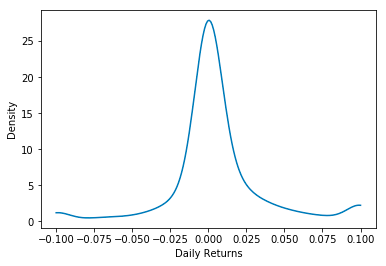
This code creates a density plot for a specific dataset of daily returns. It first defines a function called density_plot that takes in the dataset as a parameter. Within this function, it uses the gaussian_kde function from the scipy.stats library to create a density estimation for the data. The range of values for the density estimation is determined by the minimum and maximum values in the dataset, with 200 evenly spaced points in between. A covariance factor of 0.25 is set for the density estimation, and then the covariance is computed. The plt.plot function from the matplotlib library is then used to create the actual density plot, plotting the data values against the density estimation. The x-axis is labeled as Daily Returns and the y-axis as Density. Finally, the plot is shown using the plt.show function. The last two lines of code, starting with test = frames[20040108] and ending with density_plottest[DlyReturn], are used to test and visualize the density plot for a specific date in this case, January 8, 2004. The data for that specific date is extracted from the frames dataset and then a wins function is applied to it. This function assigns any values below -0.1 to -0.1 and any values above 0.1 to the value 0.1, essentially limiting the range of values for the dataset. This updated dataset is then passed into the density_plot function to create the density plot for that specific date. This allows for visualizing the distribution of returns for a specific date, compared to the overall dataset.
Exploring Factor Exposures and Estimating Factor Returns
In our analysis, we refer to a key formula for calculating returns:
Return of asset i at time t equals the summation from j equals 1 to k of the product of Factor Exposure of asset i for factor j at time t minus 2 and Factor Return for factor j at time t.
Here, i ranges from 1 to N, representing the total number of assets, and j ranges from 1 to k, indicating the total number of factors.
In simpler terms, the Return of asset i at time t is determined by multiplying each Factor Exposure of asset i for a specific factor at time t minus 2 by the corresponding Factor Return for that factor at time t, and then summing these products for all factors.
With the factor exposures derived from the Barra data and the known returns, it’s feasible to estimate the factor returns. This notebook focuses on using the Ordinary Least Squares (OLS) method for this estimation. In this method, we use the Factor Exposure of asset i for factor j at time t minus 2 as the independent variable and the Return of asset i at time t as the dependent variable to calculate the Factor Return for factor j at time t.
def get_formula(factors, Y):
    L = ["0"]
    L.extend(factors)
    return Y + " ~ " + " + ".join(L)

def factors_from_names(n):
    return list(filter(lambda x: "USFASTD_" in x, n))

def estimate_factor_returns(df):
    ## build universe based on filters
    estu = df.loc[df.IssuerMarketCap > 1e9].copy(deep=True)

    ## winsorize returns for fitting
    estu['DlyReturn'] = wins(estu['DlyReturn'], -0.25, 0.25)

    all_factors = factors_from_names(list(df))
    form = get_formula(all_factors, "DlyReturn")
    model = ols(form, data=estu)
    results = model.fit()
    return results
This code is designed to estimate factor returns using Ordinary Least Squares OLS regression. The first function, get_formula, takes in a list of factors and a dependent variable, and returns a formula for the OLS regression. The second function, factors_from_names, filters out all factors that do not contain the string USFASTD_ and returns a list of the remaining factors. The main function, estimate_factor_returns, first creates a copy of the given dataframe, limiting it to only include data from companies with a market capitalization above 1 billion dollars. It then applies a winsorization process on the daily returns, which means it limits the returns to fall within a specified range. Next, it calls the factors_from_names function and assigns the returned list of factors to the variable all_factors. This list is then used as an input for the get_formula function along with the dependent variable, DlyReturn. The ols function from the statsmodels library is then called, passing in the formula and the data from the filtered universe. The results of the regression are stored in the variable results and returned at the end of the function. In summary, this code is a systematic way to estimate factor returns using OLS regression, utilizing functions to create the necessary formula and filter out relevant factors.
facret = {}

for date in frames:
    facret[date] = estimate_factor_returns(frames[date]).params
This code snippet creates an empty dictionary called facret and then iterates through a list called frames, assigning each element in the list to the variable date. Within the for loop, the code then uses the estimate_factor_returns function to calculate a set of parameter estimates based on the given date in the frames list. These parameter estimates are then assigned as values to the facret dictionary, with the corresponding date as the key. In essence, this code is creating a dictionary that maps each date in the frames list to its respective factor return estimates.
my_dates = sorted(list(map(lambda date: pd.to_datetime(date, format='%Y%m%d'), frames.keys())))This code sorts a list of dates by converting each date from a string with the format %Y%m%d into a datetime object using the pd.to_datetime function. It does this by first applying the map function to the frames.keys list, which creates a new list by executing the pd.to_datetime function on each element in frames.keys. The result is then passed to the sorted function, which arranges the dates in ascending order. The sorted dates are stored in the my_dates variable, which can then be used for further processing. Overall, this code is useful for organizing dates in a dataset and being able to easily access and work with them in chronological order.
Download the source code from the link in the comment section.
