Optimizing Portfolio Performance: A Deep Dive into Mean-Variance and Risk Management-Chapter 4

Data-Driven Strategies for Portfolio Simulation, Risk-Adjusted Returns, and Efficient Frontier Construction in Algorithmic Trading

Sep 27, 2024

∙ Paid

We’re going to explore mean-variance analysis and risk management strategies essential for algorithmic trading in this chapter. We simulate a variety of portfolios based on returns, volatility, and the Sharpe ratio using Python libraries such as Pandas, NumPy, and SciPy. Traders should be able to make informed decisions in a data-driven, systematic way by building optimal portfolios that balance risk and return. We examine how different asset allocations can lead to better financial results with simulations and statistics.

The Kelly criterion and efficient frontier construction help determine the best asset allocations for maximizing returns and minimizing risk. Set up a simulation environment, retrieve financial data, and optimize portfolios for specific investment goals in this chapter. These methods lay the foundation for developing robust, algorithmic trading strategies whether you’re trying to minimize risk or get the best returns.

Source code at the end!

import warnings

import pandas as pd  
import numpy as np
from numpy.random import random, uniform, normal, dirichlet, choice
from numpy.linalg import inv

from scipy.optimize import minimize

import pandas_datareader.data as web
from itertools import repeat, product
import matplotlib.pyplot as plt
import seaborn as sns

This code snippet establishes an environment for data analysis and optimization by importing essential libraries for data manipulation, random number generation, and plotting. It begins with the warnings module, which controls warning messages during execution, helping to reduce output clutter. Pandas and NumPy are imported next; Pandas is used for handling structured data in DataFrames, facilitating manipulation and analysis of tabular data, while NumPy enables numerical operations, particularly with arrays and mathematical computations.

Specific functions from NumPy, such as random, uniform, normal, dirichlet, and choice, are imported to generate random numbers from various distributions, including Gaussian and uniform distributions. The code also imports inv from numpy.linalg for linear algebra functions like matrix inversion. The minimize function from scipy.optimize is included to perform optimization tasks, essential for finding the minimum of a function in data science and machine learning.

Additionally, pandas_datareader is imported to access financial data from online sources, making it easy to retrieve stock prices and economic data. The itertools modules repeat and product are included for creating iterable objects, with product being useful for generating combinations through the Cartesian product of input iterables. Finally, matplotlib.pyplot and seaborn are imported for data visualization, with Matplotlib serving as a foundational plotting library in Python, and Seaborn providing a higher-level interface for more aesthetically pleasing statistical graphics. This setup is standard for a data analysis workflow, involving data manipulation, statistical analysis, and result visualization.

Thanks for reading Onepagecode! This post is public so feel free to share it.

plt.style.use('fivethirtyeight')
np.random.seed(42)
pd.set_option('display.float_format', lambda x: '%.3f' % x)
%matplotlib inline
%config InlineBackend.figure_format = 'retina'
warnings.filterwarnings('ignore')

This code sets up the environment for data visualization using Matplotlib, NumPy, and configuration for Pandas. It applies the FiveThirtyEight style to plots for a professional look, sets the seed for NumPy’s random number generator to ensure reproducibility, and configures Pandas to display floating-point numbers with three decimal places for better readability. The code also enables Matplotlib plots to be displayed directly within a Jupyter Notebook and enhances plot resolution for high-definition displays. Additionally, it suppresses warning messages to keep the output clean. These configurations improve visual clarity and consistency in data presentation while maintaining reproducibility in random processes.

cmap = sns.diverging_palette(10, 240, n=9, as_cmap=True)

This line of code uses the Seaborn library to create a diverging color palette. It employs the sns.diverging_palette function to generate a color palette that transitions from hue 10, a light color, to hue 240, a dark blue. The argument n=9 specifies the creation of nine distinct colors, which enhances visual differentiation in data representations. The option as_cmap=True indicates that the output will be a colormap object, allowing for direct use in plotting functions that accept colormaps. This results in a nine-step color gradient suitable for highlighting differences in data values.

with pd.HDFStore('../../data/assets.h5') as store:
    sp500_stocks = store['sp500/stocks'].index 
    prices = store['quandl/wiki/prices'].adj_close.unstack('ticker').filter(sp500_stocks).sample(n=50, axis=1)

This code uses the Pandas library to manipulate an HDF5 file, a format designed for efficient data storage. It opens the HDF5 store at ../../data/assets.h5 within a context manager, ensuring proper closure of the file. Inside this block, it retrieves the index of the DataFrame at sp500/stocks, which contains S&P 500 stock identifiers, and stores it in the variable sp500_stocks. It then accesses another DataFrame at quandl/wiki/prices and extracts the adj_close column, which shows adjusted closing prices for stocks. The unstack function reshapes this DataFrame, creating separate columns for each stock ticker while maintaining dates as the index. The filter method is applied to include only the columns that correspond to the tickers in sp500_stocks. Finally, it randomly selects 50 columns from this filtered DataFrame, resulting in a smaller DataFrame with adjusted closing prices for a random selection of S&P 500 stocks for further analysis or visualization.

start = 1988
end = 2017

Two variables, start and end, are defined to hold integer values. Start is assigned the value 1988, and end is assigned the value 2017. This setup represents a range of years, which can be used for iterating over dates, filtering data, or defining a period for analysis. The start variable indicates the beginning of the period, while the end variable indicates its conclusion. These values can be utilized later in the code for computations, conditions, or loops involving the years between and including these two points.

monthly_returns = prices.loc[f'{start}':f'{end}'].resample('M').last().pct_change().dropna(how='all')
monthly_returns = monthly_returns.dropna(axis=1)
monthly_returns.info()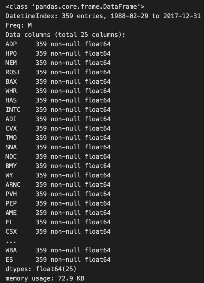

The code processes a DataFrame of stock prices to calculate monthly returns for a specified date range. It filters the DataFrame to include only the entries between the defined start and end dates, then applies the resample function to group the data by month and retrieve the last price of each month. The percentage change between these last prices for consecutive months is computed to determine the monthly returns. Rows with all NaN values are removed to retain only valid data.

Next, the code further cleans the DataFrame by dropping any columns that contain only NaN values to focus the analysis on stocks with available return data. Finally, the code provides a summary of the resulting DataFrame, which has 359 entries covering the period from February 29, 1988, to December 31, 2017, with 25 columns representing different stocks, all containing non-null float64 data types. This indicates that monthly returns for all stocks are complete for the entire date range, with no missing data. The DataFrame’s memory usage is noted at 72.9 KB, suggesting efficient storage.

n_obs, n_assets = monthly_returns.shape
n_assets, n_obs

The code snippet n_obs, n_assets = monthly_returns.shape extracts the dimensions of the monthly_returns array, which is a 2D NumPy array representing asset returns over multiple time periods, typically months. The shape attribute provides a tuple indicating the number of rows and columns in the array, where n_obs is the number of observations or time periods and n_assets is the number of assets being analyzed. In this case, the output (25, 359) indicates there are 25 observations and 359 assets, meaning the dataset contains monthly return data for 359 assets over a span of 25 months. Understanding these dimensions is important for further calculations in Mean-Variance Optimization, such as constructing the covariance matrix to assess risk associated with different asset combinations. This code snippet is a crucial step in preparing the data for financial analysis and optimization.

NUM_PF = 100000 # no of portfolios to simulate

This line defines a constant NUM_PF with a value of 100000, which represents the total number of portfolios to simulate. By placing this constant at the top of the code, it improves readability and maintainability. If you need to change the number of portfolios, you can simply update this line without searching through the code.

x0 = uniform(-1, 1, n_assets)
x0 /= np.sum(np.abs(x0))

This snippet creates an array x0 filled with random values sampled from a uniform distribution between -1 and 1 for n_assets, which is the number of assets. It then normalizes x0 by dividing each element by the sum of the absolute values of all elements. This adjustment ensures the total contribution of the values equals 1 in terms of their absolute values. Normalization is beneficial in financial applications, such as portfolio allocation, as it allows the values to represent proportions of a total while maintaining the relative proportions of the asset values. The resulting array will have a sum of absolute values equal to one.

periods_per_year = round(monthly_returns.resample('A').size().mean())
periods_per_year

The code calculates the average number of periods per year using monthly returns data. It resamples the data to an annual frequency, grouping it by year, and uses the size function to count the entries for each year to determine the number of monthly returns available. The mean function then computes the average number of monthly returns across all years. The output is 12, indicating that there are, on average, 12 monthly returns per year, which aligns with the expected number of months in a year. This suggests the dataset is complete and contains data for each month. The calculation is important for the Mean-Variance Optimization project, as it establishes the frequency of returns for further analyses that influence asset allocation based on risk and return profiles.

mean_returns = monthly_returns.mean()
cov_matrix = monthly_returns.cov()
precision_matrix = pd.DataFrame(inv(cov_matrix), index=stocks, columns=stocks)

You are calculating key statistics from a DataFrame called monthly_returns, which includes the returns of different stocks over time. The mean_returns is computed using the mean method to determine the average return for each stock, resulting in a Series indexed by stock names with corresponding average returns. The cov_matrix is calculated using the cov method to generate the covariance matrix, which measures how two stocks move together, helping you understand their relationships. The cov_matrix is a square DataFrame with stock names as both row and column labels, where each entry indicates the covariance between the returns of two stocks. Finally, the covariance matrix is transformed into a precision matrix by computing its inverse and creating a new DataFrame with stock names as labels. This precision matrix provides valuable insights for minimizing risk in portfolio management.

treasury_10yr_monthly = (web.DataReader('DGS10', 'fred', start, end)
                         .resample('M')
                         .last()
                         .div(periods_per_year)
                         .div(100)
                         .squeeze())

This code snippet retrieves 10-year Treasury yield data from the Federal Reserve Economic Data using the web.DataReader method, specifying the ticker DGS10 for the 10-year Treasury rate along with the desired start and end dates. The data is then resampled to a monthly frequency, taking the last entry for each month. To normalize the data, it is divided by periods per year, likely converting it to a specific annualized scale, and then divided by 100 to convert percentage values to decimals. Finally, the squeeze method simplifies the data structure to a Series if it is one-dimensional, resulting in a clean monthly dataset of 10-year Treasury yields ready for analysis.

rf_rate = treasury_10yr_monthly.mean()

This code calculates the average value of the treasury_10yr_monthly data, which contains the monthly yields of 10-year Treasury bonds. The mean function computes the average of these values, and the result is stored in the rf_rate variable, representing the risk-free rate for this investment duration. This method is commonly used in finance to establish a baseline interest rate for models and analyses.

alpha = np.full(shape=n_assets, fill_value=.01)
weights = dirichlet(alpha=alpha, size=NUM_PF)
weights *= choice([-1, 1], size=weights.shape)
weights.shape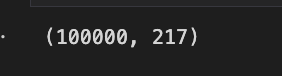

The code initializes an array named alpha with a shape determined by n_assets, where each element is set to 0.01. This array is used as a parameter for generating random weights through the Dirichlet distribution, which ensures that the weights sum to one, a common requirement in portfolio optimization. The dirichlet function is invoked with alpha and produces a specified number of portfolios, defined by NUM_PF, resulting in a 2D array of weights with each row representing a different portfolio.

Subsequently, the code adjusts the weights by multiplying each by either -1 or 1, randomly chosen, allowing for negative weights that indicate short positions in a portfolio. The final output, the shape of the weights array, is (100000, 217), signifying the generation of 100,000 portfolios, each with weights for 217 different assets. This output confirms the successful creation of a vast array of diverse portfolios, crucial for analyzing various investment strategies in mean-variance optimization.

def simulate_portfolios(mean_ret, cov, rf_rate=rf_rate, short=True):
    alpha = np.full(shape=n_assets, fill_value=.025)
    weights = dirichlet(alpha=alpha, size=NUM_PF)
    weights *= choice([-1, 1], size=weights.shape)

    returns = weights @ mean_ret.values + 1
    returns = returns ** periods_per_year - 1
    std = (weights @ monthly_returns.T).std(1)
    std *= np.sqrt(periods_per_year)
    sharpe = (returns - rf_rate) / std

    return pd.DataFrame({'Annualized Standard Deviation': std,
                         'Annualized Returns': returns,
                         'Sharpe Ratio': sharpe}), weights

This function simulates investment portfolios using a mean return vector and a covariance matrix of asset returns. It begins by creating an alpha array filled with 0.025 to generate Dirichlet distributions. Weights are produced from the Dirichlet distribution, resulting in random weights that sum to one for each portfolio. These weights can be either positive or negative based on a random choice, allowing for short positions when the short argument is set to true.

The function calculates the annualized returns for each portfolio by taking the dot product of the portfolio weights and the mean returns, adjusting for compounding over a year. It then computes the annualized standard deviation, or risk, of the portfolios, which involves determining the standard deviation of monthly returns based on the weights and scaling this figure for the entire year.

Finally, the Sharpe ratio is calculated for each portfolio, assessing risk-adjusted returns by subtracting the risk-free rate from the annualized returns and dividing by the annualized standard deviation. The function returns a Pandas DataFrame that includes the annualized standard deviation, returns, Sharpe ratio, and weights for each portfolio.

simul_perf, simul_wt = simulate_portfolios(mean_returns, cov_matrix, short=False)

This line of code calls the simulate_portfolios function, which creates simulated investment portfolios based on the inputs mean_returns and cov_matrix. Mean_returns contains the average expected returns for various assets, indicating their potential performance over time. The cov_matrix shows how the asset returns move together, which is critical for understanding the portfolio’s risk and return characteristics. The short argument is set to false, meaning short-selling is not permitted, resulting in portfolios that only contain long positions. The function returns two items: simul_perf and simul_wt. Simul_perf provides performance metrics of the simulated portfolios, such as expected returns or risk-adjusted measures. Simul_wt contains the weights of each asset in the portfolios, essential for risk management and performance evaluation.

# pandas 0.24 will fix bug with colorbars: https://github.com/pandas-dev/pandas/pull/20446
ax = simul_perf.plot.scatter(x=0, y=1, c=2,
                             cmap='RdBu',
                             alpha=0.5, figsize=(14, 9), colorbar=False,
                             title=f'{NUM_PF:,d} Simulated Portfolios')

max_sharpe_idx = simul_perf.iloc[:, 2].idxmax()
sd, r = simul_perf.iloc[max_sharpe_idx, :2].values
ax.scatter(sd, r, marker='*', color='darkblue',
           s=500, label='Max. Sharpe Ratio')

min_vol_idx = simul_perf.iloc[:, 0].idxmin()
sd, r = simul_perf.iloc[min_vol_idx, :2].values
ax.scatter(sd, r, marker='*', color='green', s=500, label='Min Volatility')
plt.legend(labelspacing=1, loc='upper left')
plt.tight_layout()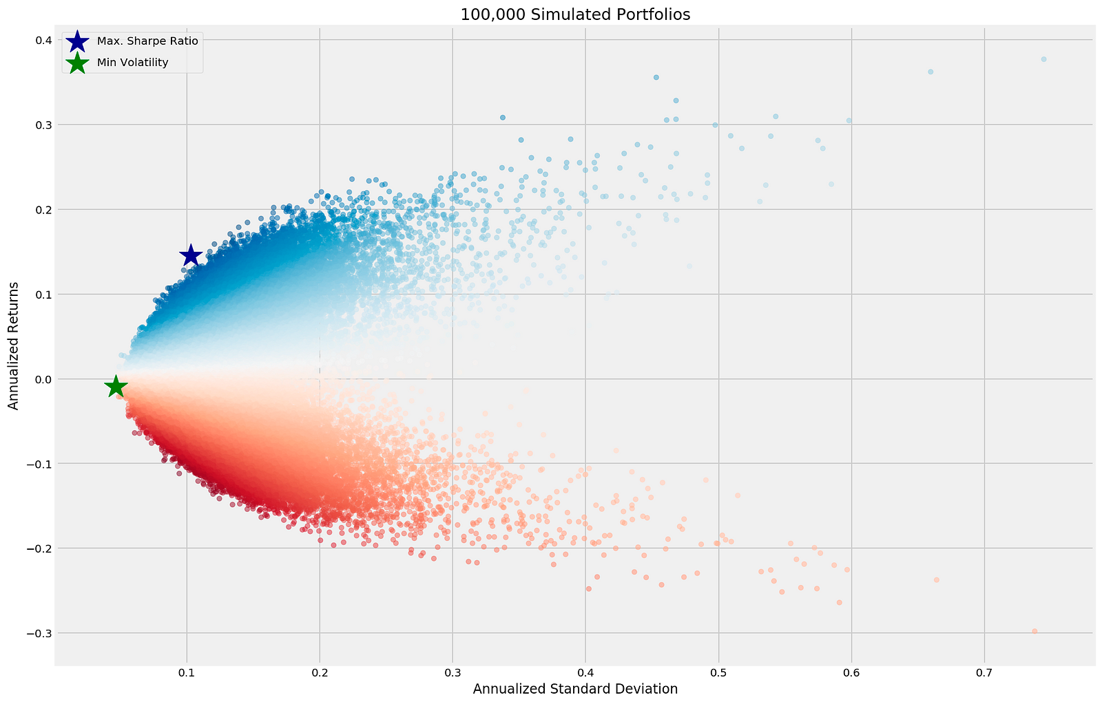

The code snippet generates a scatter plot that visualizes the results of a mean-variance optimization simulation with 100,000 simulated portfolios based on their annualized returns and standard deviations. The x-axis represents annualized standard deviation, indicating portfolio risk, while the y-axis shows annualized returns, reflecting potential profit. Each point corresponds to a different portfolio, with colors ranging from blue to red to signify varying returns.

The code highlights two key portfolios: the one with the maximum Sharpe ratio, marked by a dark blue star to indicate the best return per unit of risk, and the one with minimum volatility, indicated by a green star as the least risky option. These portfolios are essential for investors aiming to optimize their risk-return balance.

The output plot illustrates the distribution of simulated portfolios and uses a gradient color scheme to emphasize the risk-return relationship. The legend in the upper left corner clarifies the markers for the maximum Sharpe ratio and minimum volatility portfolios, facilitating understanding of their significance within the simulation. The plot effectively conveys the results of the optimization process, enabling quick assessment of portfolio selection trade-offs.

def portfolio_std(wt, rt=None, cov=None):
    """Annualized PF standard deviation"""
    return np.sqrt(wt @ cov @ wt * periods_per_year)

The portfolio_std function calculates the annualized standard deviation of a portfolio, which measures risk. The primary input is a vector of asset weights, indicating the proportion of the total investment in each asset. Optional parameters include returns, which are not utilized in this calculation, and the covariance matrix of asset returns, which shows how different assets’ returns move together.

The calculation uses matrix multiplication. First, the function computes portfolio variance by multiplying the weight vector with the covariance matrix, generating a new vector that reflects the relationship between asset returns based on their allocations. This result is then multiplied by the weight vector again to finalize the variance calculation. The variance is multiplied by periods per year to annualize the standard deviation, adjusting it from the original period to a yearly perspective. Finally, taking the square root of this value yields the portfolio’s standard deviation, providing an indication of how much the portfolio’s returns may deviate from the average. This function allows for a straightforward assessment of a portfolio’s risk level based on asset allocation and the covariance of returns.

def portfolio_returns(wt, rt=None, cov=None):
    """Annualized PF returns"""
    return (wt @ rt + 1) ** periods_per_year - 1

This function calculates the annualized returns of a portfolio based on asset weights and their returns. It requires three parameters: weights representing the investment proportions for each asset, periodic returns of the assets, and a covariance parameter that is currently unused but may be for future expansions.

The main calculation performed by the function is the expression (wt @ rt + 1) ** periods_per_year — 1. The matrix multiplication operator computes the weighted sum of returns, converting this sum into a growth factor by adding one. Raising this growth factor to the power of the number of periods in a year annualizes the returns, and subtracting one converts the result into a percentage. By providing the correct weights and returns, you can obtain the scaled annualized return of your portfolio. The code should include additional error handling for missing values in the returns and covariance parameters to improve its robustness.

def portfolio_performance(wt, rt, cov):
    """Annualized PF returns & standard deviation"""
    r = portfolio_returns(wt, rt=rt)
    sd = portfolio_std(wt, cov=cov)
    return r, sd

The function portfolio_performance calculates the annualized returns and standard deviation of a financial portfolio. It takes three arguments: wt for the weights of different assets, rt for the returns of those assets, and cov for the covariance matrix that reflects how asset returns move together. It first computes the overall portfolio return by calling the portfolio_returns function with the weights and returns, storing the result in the variable r. Next, it calculates the portfolio’s standard deviation using the portfolio_std function with the same weights and the covariance matrix, storing this value in sd. The function then returns a tuple containing the annualized return and the standard deviation, providing a concise view of the portfolio’s performance metrics.

def neg_sharpe_ratio(weights, mean_ret, cov):
    r, sd = portfolio_performance(weights, mean_ret, cov)
    return -(r - rf_rate) / sd

The neg_sharpe_ratio function computes the negative Sharpe ratio for a set of portfolio weights, allowing for risk minimization in optimization tasks. It accepts three parameters: weights, which represent the distribution of assets; mean_ret, the expected returns of those assets; and cov, the covariance matrix of the asset returns indicating risk. The function invokes another function, portfolio_performance, to determine the portfolio’s expected return and standard deviation based on the provided parameters. It then calculates the negative Sharpe ratio using the formula — (r — rf_rate) / sd, where rf_rate is the risk-free rate defined elsewhere in the code. This inverted value assists in assessing the risk-adjusted performance of investments for optimization purposes.

weight_constraint = {'type': 'eq', 
                     'fun': lambda x: np.sum(np.abs(x)) - 1}

This code snippet defines a weight constraint for an optimization problem, requiring the sum of the absolute values of the elements in an array to equal one. The weight_constraint is a dictionary containing two main components. First, the type is set to eq, signifying that this constraint must be satisfied exactly rather than being merely less than or greater than a particular value. Second, the function is defined using a lambda function that takes an input x. It computes the sum of the absolute values of the elements in x and subtracts one. For the constraint to be valid, the output of this function must be zero, ensuring that the total of the absolute values equals one. This constraint is particularly useful for normalizing weights in optimization, maintaining a specific scale.

def max_sharpe_ratio(mean_ret, cov, short=True):
    return minimize(fun=neg_sharpe_ratio,
                    x0=x0,
                    args=(mean_ret, cov),
                    method='SLSQP',
                    bounds=((-1 if short else 0, 1),) * n_assets,
                    constraints=weight_constraint,
                    options={'tol':1e-10, 'maxiter':1e4})

The max_sharpe_ratio function optimizes the Sharpe ratio of a portfolio, which measures risk-adjusted return. The function takes mean_ret, representing the expected returns of the assets, and cov, the covariance matrix indicating the risk associated with asset returns, as inputs. The short parameter determines if short-selling is allowed; if set to True, the function accepts negative weights; if False, only non-negative weights are permitted.

The function employs the minimize function from the SciPy library to minimize an objective function called neg_sharpe_ratio, which calculates the negative of the Sharpe ratio to facilitate maximization. The x0 variable serves as the initial guess for asset weights. The arguments mean_ret and cov are passed to neg_sharpe_ratio during optimization. The optimization method used is the Sequential Least Squares Quadratic Programming algorithm, suitable for bounded constraint problems.

The bounds argument establishes limits for asset weights; allowed ranges vary from -1 to 1 for short-selling and from 0 to 1 when it is not permitted. Additionally, constraints are applied to the portfolio weights, ensuring compliance with specific conditions. The options parameter controls the tolerance level and maximum iterations for the optimization process, ensuring precision and preventing indefinite execution. Ultimately, this function aims to determine the optimal asset weights in a portfolio for maximizing the Sharpe ratio while accommodating short-selling if desired.

def min_vol_target(mean_ret, cov, target, short=True):

    def ret_(wt):
        return portfolio_returns(wt, mean_ret)

    constraints = [{'type': 'eq', 'fun': lambda x: ret_(x) - target},
                   weight_constraint]

    bounds = ((-1 if short else 0, 1),) * n_assets
    return minimize(portfolio_std,
                    x0=x0,
                    args=(mean_ret, cov),
                    method='SLSQP',
                    bounds=bounds,
                    constraints=constraints,
                    options={'tol': 1e-10, 'maxiter': 1e4})

The function min_vol_target minimizes portfolio volatility while achieving a specified target return. It takes four arguments: mean_ret, which represents expected asset returns; cov, the covariance matrix illustrating the movement of asset returns; target, the desired return; and short, a boolean indicating whether short selling is permitted.

Within the function, there is a nested function ret_ that calculates portfolio return based on asset weights. It utilizes an external function portfolio_returns to compute total returns based on the weights and mean returns. Constraints are established to ensure the solution meets the target return. The first constraint ensures the portfolio return equals the specified target, while the second, referred to as weight_constraint, maintains that the weights sum to a predefined value.

Bounds for asset weights are defined based on the short parameter. If short is true, weights can range down to -1, allowing shorting; if false, weights must be 0 or higher, prohibiting shorting. Each asset thus has identical bounds.

The function then calls minimize, likely from a library such as SciPy, to minimize portfolio volatility, using another function portfolio_std. Optimization starts with an initial guess for the weights and employs the Sequential Least Squares Programming method. Options are set for tight tolerance and a maximum number of iterations for improved accuracy.

This function systematically identifies the optimal asset distribution to meet the target return while minimizing risk.

def min_vol(mean_ret, cov, short=True):
    bounds = ((-1 if short else 0, 1),) * n_assets

    return minimize(fun=portfolio_std,
                    x0=x0,
                    args=(mean_ret, cov),
                    method='SLSQP',
                    bounds=bounds,
                    constraints=weight_constraint,
                    options={'tol': 1e-10, 'maxiter': 1e4})

The min_vol function identifies the minimum volatility portfolio based on expected returns, covariance, and short selling preferences. It begins by setting bounds for asset weights. If short selling is allowed, weights can range from -1 to 1. If not, weights are limited to 0 to 1, meaning all assets are held long. The bounds are applied for the number of assets in the portfolio.

Next, the function utilizes the minimize function from an optimization library, targeting the portfolio_std function, which calculates portfolio volatility based on the weights, mean returns, and covariance matrix. The optimization starts with an initial array of asset weights defined by x0. The function also accepts additional parameters like mean_ret and cov through the args parameter.

The optimization method employed is SLSQP, suitable for constrained problems. The bounds restrict asset weights according to short selling permissions, while a weight constraint ensures that the sum of weights equals 1, a common requirement. Finally, the optimization process is fine-tuned with options for tolerance and maximum iterations. This setup effectively determines the optimal asset allocation to minimize portfolio volatility based on the specified conditions.

def efficient_frontier(mean_ret, cov, ret_range, short=True):
    return [min_vol_target(mean_ret, cov, ret) for ret in ret_range]

The efficient_frontier function generates the efficient frontier for investment portfolios based on expected returns and the covariance of returns. It accepts three parameters: mean_ret, an array of expected returns for various assets; cov, the covariance matrix indicating how asset returns move together; and ret_range, a range of target returns for which minimum volatility needs to be determined. It also includes a short parameter, indicating whether short selling is allowed, set to true. The function uses a list comprehension to call min_vol_target for each target return in ret_range, calculating the minimum volatility portfolio for each. The resulting list shows the volatility associated with different expected return levels, which is essential for portfolio optimization.

simul_perf, simul_wt = simulate_portfolios(mean_returns, cov_matrix, short=True)

This line of code calls the function simulate_portfolios, which generates portfolio simulations based on input parameters. The parameter mean_returns contains the average returns for different assets, representing the expected return for each asset. The cov_matrix is the covariance matrix that shows how returns on various assets move together, which is crucial for assessing risk in a portfolio. The function has a parameter named short set to True, indicating that the simulation allows for short-selling, enabling portfolios to include positions that bet on a decline in asset prices. The outputs simul_perf and simul_wt store performance information for each simulated portfolio, including returns or risk metrics, and the weights assigned to assets, respectively, detailing the allocation of each asset in the portfolios.

print(simul_perf.describe())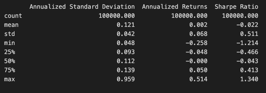

The code snippet print(simul_perf.describe()) generates a statistical summary of the simul_perf DataFrame, which contains performance metrics from a Mean-Variance Optimization project. It provides key statistics for three financial metrics: Annualized Standard Deviation, Annualized Returns, and Sharpe Ratio.

The Annualized Standard Deviation column reflects the volatility of returns, with a mean value of 0.121 indicating low average volatility. The maximum value of 0.959 shows instances of high volatility, while a standard deviation of 0.042 suggests slight variations around the mean. The minimum value of 0.048 indicates periods of very low volatility.

The Annualized Returns column shows the average returns from the investment strategy. The mean return is 0.002, signifying modest average returns. The maximum return of 0.514 indicates instances of significantly higher returns, while the minimum of -0.258 suggests some scenarios resulted in losses. The standard deviation of 0.068 reflects variability in returns during the simulation.

The Sharpe Ratio column measures risk-adjusted return, with a mean of -0.022 indicating that, on average, returns do not compensate for the risk taken. However, a maximum Sharpe Ratio of 1.340 suggests some scenarios significantly exceed the risk, while the minimum of -1.214 highlights poor performance instances.

This statistical summary offers a clear view of the investment strategy’s performance characteristics, aiding in the assessment of its risk and return profile, and informing decisions on portfolio optimization and risk management.

simul_max_sharpe = simul_perf.iloc[:, 2].idxmax()
simul_perf.iloc[simul_max_sharpe]

The code identifies the portfolio with the highest Sharpe ratio from a DataFrame named simul_perf. It retrieves the index of the maximum value from the third column, which represents the Sharpe ratios. The Sharpe ratio measures risk-adjusted return, indicating the excess return for the volatility of a riskier asset. Using the index, the code extracts the entire row corresponding to the portfolio with the highest Sharpe ratio, which includes essential performance metrics like annualized standard deviation, annualized returns, and the Sharpe ratio itself.

The output shows an annualized standard deviation of 0.099, reflecting the portfolio’s risk level, and annualized returns of 0.136, indicating the expected return over the year. The Sharpe ratio is 1.340, suggesting a favorable return compared to its risk, as a ratio above 1 is considered good. The output also confirms the index name and data type of the analyzed data. This code effectively identifies and presents the optimal portfolio based on the Sharpe ratio, supporting investment decision-making.

max_sharpe_pf = max_sharpe_ratio(mean_returns, cov_matrix, short=False)
max_sharpe_perf = portfolio_performance(max_sharpe_pf.x, mean_returns, cov_matrix)

This snippet focuses on optimizing a portfolio to achieve the maximum Sharpe ratio, which measures risk-adjusted return. The first line calls the max_sharpe_ratio function with mean_returns and cov_matrix as key arguments, where mean_returns indicates expected asset returns and cov_matrix conveys how asset returns interact. The short parameter is set to False, meaning short-selling is not permitted.

The second line takes the optimal asset allocation from the first line and uses it, along with mean_returns and cov_matrix, to call the portfolio_performance function. This function likely calculates various performance metrics, such as expected return, volatility, and the Sharpe ratio. Together, these lines determine the best asset allocation for maximizing risk-adjusted return and compute the performance metrics for that portfolio.

r, sd = max_sharpe_perf
pd.Series({'ret': r, 'sd': sd, 'sr': (r-rf_rate)/sd})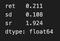

The code snippet extracts the maximum Sharpe ratio performance from a variable named max_sharpe_perf, which contains two values: return and standard deviation. A Pandas Series summarizes key performance metrics of a portfolio, showing a return of 0.211, or 21.1%, and a standard deviation of 0.108, indicating the portfolio’s risk with returns varying by about 10.8%. The Sharpe ratio is calculated using the formula (return — risk-free rate) / standard deviation, resulting in approximately 1.924. This suggests a favorable return per unit of risk, as a Sharpe ratio above 1 is generally seen as good. The Series is stored as float64, confirming the values are floating-point numbers, typical for financial metrics. This summary enables investors to assess the performance and risk profile of the portfolio in the context of mean-variance optimization.

min_vol_pf = min_vol(mean_returns, cov_matrix, short=False)
min_vol_perf = portfolio_performance(min_vol_pf.x, mean_returns, cov_matrix)

This code calculates the optimal minimal volatility portfolio using two functions: min_vol and portfolio_performance. The function min_vol takes expected returns and the covariance matrix of asset returns as inputs to determine the asset weights that minimize the portfolio’s volatility. The parameter short is set to false, which means short-selling is not allowed, ensuring all asset weights are non-negative. The output of this function is an array of weights indicating how to allocate assets for minimum volatility.

The next step involves the function portfolio_performance, which evaluates the performance metrics of the minimum volatility portfolio using the asset weights obtained from min_vol. This function typically returns values such as expected return, volatility, and possibly the Sharpe ratio, providing insights into the portfolio’s expected performance based on the input data.

ret_range = np.linspace(0, simul_perf.iloc[:, 1].max() * 1.1, 25)
eff_pf = efficient_frontier(mean_returns, cov_matrix, ret_range,short=False)

This code constructs an efficient frontier, which visually represents the relationship between risk and return for various portfolios. It begins by creating a return range using np.linspace, generating an array of 25 evenly spaced values from 0 to 10% above the maximum performance metric in the second column of the simul_perf DataFrame. This range serves as potential return targets for the portfolios. The return range is then passed to the efficient_frontier function, along with mean_returns and cov_matrix, which likely represent expected returns and the covariance matrix of different assets. The short=False argument indicates that short selling is not permitted in the portfolio construction.

fig, ax = plt.subplots()
simul_perf.plot.scatter(x=0, y=1, c=2, ax=ax,
                                 cmap='RdBu',
                                 alpha=0.5, figsize=(14, 9), colorbar=False,
                                 title='Mean-Variance Efficient Frontier')

r, sd = max_sharpe_perf
ax.scatter(sd, r, marker='*', color='r', s=500, label='Max Sharpe Ratio PF')

r, sd = min_vol_perf
ax.scatter(sd, r, marker='*', color='g', s=500, label='Min Volatility PF')

kelly_wt = precision_matrix.dot(mean_returns).values
kelly_wt /= np.sum(np.abs(kelly_wt))
r, sd = portfolio_performance(kelly_wt, mean_returns, cov_matrix)
ax.scatter(sd, r, marker='*', color='darkgrey', s=500, label='Kelly PF')

std = monthly_returns.std()
std /= std.sum()
r, sd = portfolio_performance(std, mean_returns, cov_matrix)
ax.scatter(sd, r, marker='*', color='y', s=500, label='Risk Parity PF')

r, sd = portfolio_performance(np.full(n_assets, 1/n_assets), mean_returns, cov_matrix)
ax.scatter(sd, r, marker='*', color='blue', s=500, label='1/n PF')

ax.plot([p['fun'] for p in eff_pf], ret_range, 
        linestyle='--', lw=3, color='darkgrey', label='Efficient Frontier')
ax.legend(labelspacing=0.8)
fig.tight_layout();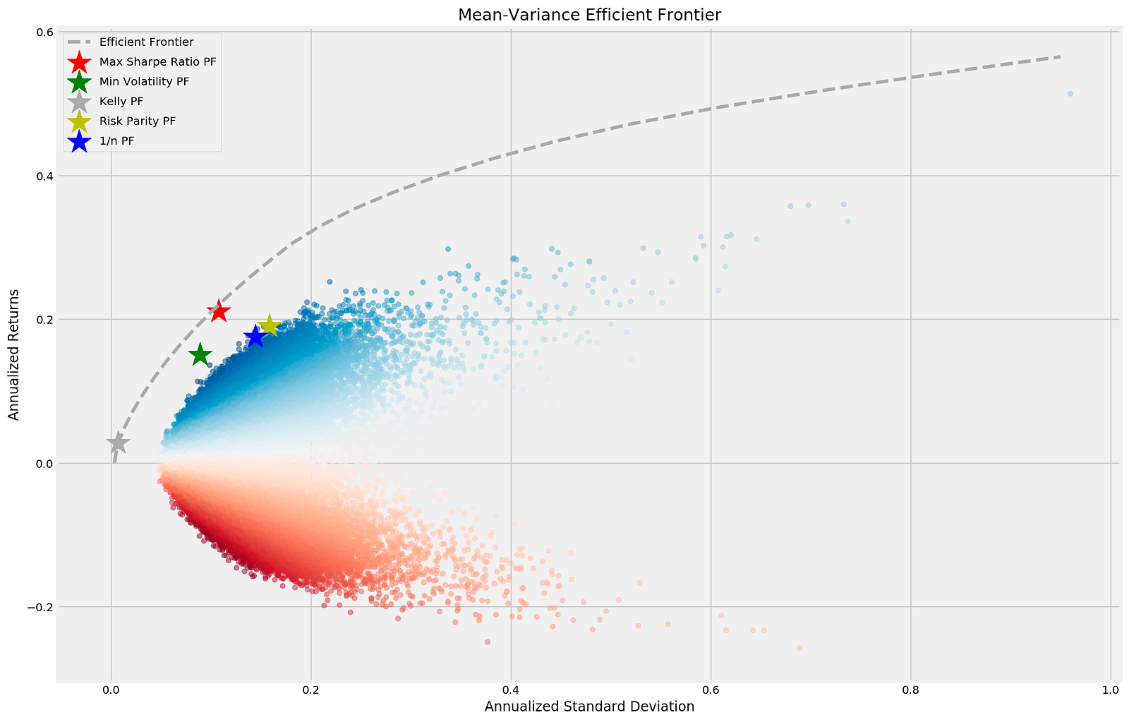

\The code generates a scatter plot that visualizes the Mean-Variance Efficient Frontier, an essential concept in portfolio optimization. Using Matplotlib, it depicts the annualized standard deviation (risk) on the x-axis and annualized returns on the y-axis for various portfolios. The scatter plot is based on the simul_perf DataFrame, with colors indicating the performance of different portfolios and adjusted transparency using the alpha parameter. The title of the plot is Mean-Variance Efficient Frontier.

Key portfolios are highlighted: the maximum Sharpe ratio portfolio is marked with a red star, representing the best return per unit of risk, while the minimum volatility portfolio is indicated by a green star, reflecting the lowest risk. The Kelly portfolio is shown in dark grey, the risk parity portfolio in yellow, and the equal-weight portfolio in blue, which allocates equal weights to all assets. The efficient frontier is represented by a dashed line, signifying the optimal portfolios that provide the highest expected return for a given level of risk, typically sloping upward to show the relationship between risk and return. The legend clarifies the different portfolios and their markers. This output effectively demonstrates the risk-return relationship for various investment strategies, facilitating the comparative analysis of portfolio performance in mean-variance optimization.

Optimizing Portfolio Performance: A Deep Dive into Mean-Variance and Risk Management-Chapter 4

Data-Driven Strategies for Portfolio Simulation, Risk-Adjusted Returns, and Efficient Frontier Construction in Algorithmic Trading

This post is for paid subscribers