

Optimizing Portfolios with Kelly Criterion and Mean-Variance Analysis
Combining Risk-Return Efficiency and Strategic Asset Allocation for Maximizing Long-Term Growth

This article explores the combination of the Kelly Criterion and Mean-Variance Optimization to enhance portfolio management strategies. The Kelly Criterion, a formula used to maximize long-term growth by determining optimal bet sizing, is applied alongside the traditional mean-variance analysis, which balances expected returns against portfolio risk. By integrating these approaches, investors can optimize their asset allocation to achieve both higher returns and more efficient risk management. The analysis leverages real market data from the S&P 500, focusing on practical applications of these techniques in financial decision-making.
Mean-Variance Optimization
import warnings

import pandas as pd
import numpy as np
from numpy.random import random, uniform, normal, dirichlet, choice
from numpy.linalg import inv

from scipy.optimize import minimize

import pandas_datareader.data as web
from itertools import repeat, product
import matplotlib.pyplot as plt
import seaborn as sns
By importing essential libraries for manipulating data, creating random numbers, and plotting, this code snippet sets up a data analysis environment. During execution, it controls warning messages, reducing output clutter. DataFrames are manipulated and analyzed with Pandas, while NumPy allows numerical operations, particularly with arrays and mathematical computations.
Random numbers from different distributions, including Gaussian and uniform distributions, are generated by imports from NumPy, including random, uniform, normal, dirichlet, and choice. For linear algebra functions such as matrix inversion, inv from numpy.linalg is also imported. Using scipy.optimize, you can perform optimization tasks, essential to machine learning and data science.
In addition, pandas_datareader can be imported to access economic data and stock prices online. Repeat and product are included in itertools modules for creating iterable objects, with product generating combinations by taking the Cartesian product of input iterables. A foundational Python plotting library Matplotlib is imported for data visualization, while Seaborn provides a more aesthetic interface for statistical graphics. Data manipulation, statistical analysis, and result visualization are all part of a standard data analysis workflow.
plt.style.use('fivethirtyeight')
np.random.seed(42)
pd.set_option('display.float_format', lambda x: '%.3f' % x)
%matplotlib inline
%config InlineBackend.figure_format = 'retina'
warnings.filterwarnings('ignore')
Using Matplotlib, NumPy, and Pandas, this code sets up the data visualization environment. For a professional look on plots, it applies the FiveThirtyEight style, sets a seed for NumPy’s random number generator, and configures Pandas to display floating-point numbers with three decimal places. It also enhances plot resolution for high-definition displays and allows Matplotlib plots to be displayed directly within Jupyter Notebooks. In addition to suppressing warning messages, these configurations ensure visual clarity and consistency in data presentation while preserving reproducibility.
cmap = sns.diverging_palette(10, 240, n=9, as_cmap=True)By using the Seaborn library, this code creates a diverging color palette that transitions from hue 10, a light color, to hue 240, a deep blue. With n=9, nine distinct colors are created, enhancing visual differentiation. As_cmap=True means the output will be a colormap object, so it can be directly used in plotting functions accepting colormaps. In this way, differences in data values are highlighted using a 9-step color gradient.
with pd.HDFStore('../../data/assets.h5') as store:
    sp500_stocks = store['sp500/stocks'].index
    prices = store['quandl/wiki/prices'].adj_close.unstack('ticker').filter(sp500_stocks).sample(n=50, axis=1)
Pandas is used to manipulate HDF5 files, which are a format designed for efficient data storage. The file is opened within a context manager and closed properly. The index of the DataFrame at sp500/stocks is stored in variable sp500_stocks in this block. A DataFrame at quandl/wiki/prices is accessed to extract adj_close, which shows adjusted closing prices. An unstack function reshapes this DataFrame by creating columns for each ticker while keeping dates as the index. By filtering, only the columns that correspond to the tickers in sp500_stocks are included. In the final step, it randomly selects 50 columns from this filtered DataFrame, resulting in an adjusted closing price DataFrame for a random selection of S&P 500 stocks.
start = 1988
end = 2017
Start and end are defined as integer variables, with 1988 assigned to start and 2017 assigned to end. With this setup, you can iterate over dates, filter data, or define a period to analyze. The start variable indicates the beginning of the period, and the end variable indicates its conclusion. Further computations, conditions, or loops involving these two points can be performed using these values.
monthly_returns = prices.loc[f'{start}':f'{end}'].resample('M').last().pct_change().dropna(how='all')
monthly_returns = monthly_returns.dropna(axis=1)
monthly_returns.info()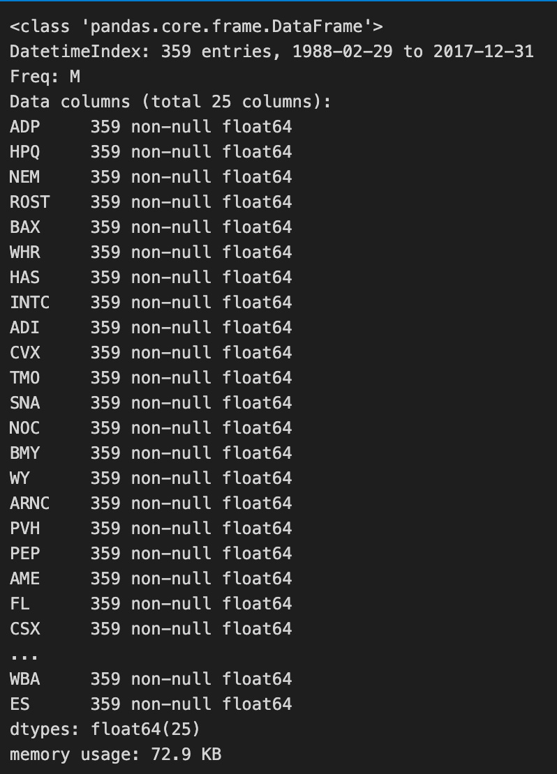
Calculates monthly returns for a specified date range from a DataFrame of stock prices. The data is filtered to include only entries between the defined start and end dates, then grouped by month and retrieved by the last price. In order to calculate monthly returns, the percentage change between these last prices over consecutive months is calculated. Rows with NaN values are removed.
By dropping columns containing only NaN values, the code further cleans the DataFrame. In addition, the code provides a summary of the DataFrame, which contains 359 entries covering the period February 29, 1988, through December 31, 2017, all of which contain non-null float64 data types representing stocks. DataFrame memory usage is noted at 72.9 KB, suggesting efficient storage of monthly returns for all stocks over the entire period. This process ensures completeness and relevance in the monthly return data used for further analysis.
stocks = monthly_returns.columnsAn Index object with all the column names is returned by the columns attribute from the DataFrame named monthly_returns. In the case that monthly_returns has different stocks in its columns, this line creates a variable stocks that stores those names.
n_obs, n_assets = monthly_returns.shape
n_assets, n_obs
With the code snippet n_obs, n_assets = monthly_returns.shape, you can extract the dimensions of the 2D NumPy array monthly_returns, which represents asset returns for several months in advance. An array’s shape attribute indicates its rows and columns, where n_obs is the number of observations or time periods and n_assets is the number of assets to analyze. A dataset with 25 observations and 359 assets contains monthly return data over a 25-month period, as indicated by output (25, 359). For further calculations in Mean-Variance Optimization, such as assessing risk associated with different asset combinations, understanding these dimensions is important. To analyze and optimize data, this code snippet is crucial.
NUM_PF = 100000 # no of portfolios to simulateBy placing this constant at the top of the code, it increases readability and maintainability. NUM_PF represents the total number of portfolios to simulate, so you don’t have to search through the code to change the number of portfolios.
x0 = uniform(-1, 1, n_assets)
x0 /= np.sum(np.abs(x0))
The array x0 is filled with random values from a uniform distribution between -1 and 1 for n_assets. By dividing the absolute values of each element by the sum of all elements, it normalizes x0, ensuring the total contribution equals 1 in absolute terms. Financial applications, such as portfolio allocation, benefit from normalization as it preserves relative proportions of asset values while representing proportions of a total.
periods_per_year = round(monthly_returns.resample('A').size().mean())
periods_per_year
A number of periods per year is calculated using monthly returns data. A number of monthly returns can be determined by resampling the data to an annual frequency, grouping it by year, and counting the entries by size. A mean function computes the average number of monthly returns. According to the output, there are 12 monthly returns per year, which is consistent with the expected number of months in a year. This indicates that the data are complete. It is important for the Mean-Variance Optimization project to calculate the frequency of returns in order to influence asset allocation based on risk and return profiles.
mean_returns = monthly_returns.mean()
cov_matrix = monthly_returns.cov()
precision_matrix = pd.DataFrame(inv(cov_matrix), index=stocks, columns=stocks)
From a DataFrame called monthly_returns, which includes returns over time, you are calculating key statistics. By using the mean method, the average return for each stock is calculated, resulting in a Series indexed by stock names. Covariance matrixes measure how two stocks move together, which can help you understand their relationships, so you calculate the cov_matrix. cov_matrix represents the covariance between the returns of two stocks, with stock names as column and row labels. By computing its inverse and creating a DataFrame with stock names as labels, the covariance matrix is transformed into a precision matrix. With this precision matrix, portfolio managers can minimize risk.
treasury_10yr_monthly = (web.DataReader('DGS10', 'fred', start, end)
                         .resample('M')
                         .last()
                         .div(periods_per_year)
                         .div(100)
                         .squeeze())
It uses the web.DataReader method to retrieve 10-year Treasury yield data from the Federal Reserve Economic Data, with the ticker DGS10 specified as well as the desired start and end dates. Each entry is taken as the last entry. Normalizing the data involves dividing it into periods per year, converting it into a specific annualized scale, and then dividing it by 100 to convert percentage values to decimals. A clean monthly dataset of 10-year Treasury yields can be produced by the squeeze method if the data structure is one-dimensional.
rf_rate = treasury_10yr_monthly.mean()It calculates the average yield of Treasury 10-year bonds based on the treasury_10yr_monthly data. These values are averaged by the mean function, and the result is stored in the rf_rate variable. A base interest rate is usually determined using this method in finance.
alpha = np.full(shape=n_assets, fill_value=.01)
weights = dirichlet(alpha=alpha, size=NUM_PF)
weights *= choice([-1, 1], size=weights.shape)
weights.shape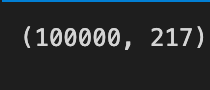
With n_assets as a shape, the code initializes an array alpha, which contains a 0.01 element for each element. Using this array as a parameter, the Dirichlet distribution generates random weights, which ensures that they sum up to one, as a standard portfolio optimization requirement. Dirichlet produces a 2D array of weights with each row representing a different portfolio based on NUM_PF.
Following that, each weight is multiplied by -1 or 1, randomly chosen, which allows for negative weights, which indicate short positions. A final output, the weights array, is (100000, 217), which signifies that 100,000 portfolios were generated with weights for 217 assets each. As a result, a vast array of diverse portfolios is created, crucial to analyzing various investment strategies.
def simulate_portfolios(mean_ret, cov, rf_rate=rf_rate, short=True):
    alpha = np.full(shape=n_assets, fill_value=.025)
    weights = dirichlet(alpha=alpha, size=NUM_PF)
    weights *= choice([-1, 1], size=weights.shape)

    returns = weights @ mean_ret.values + 1
    returns = returns ** periods_per_year - 1
    std = (weights @ monthly_returns.T).std(1)
    std *= np.sqrt(periods_per_year)
    sharpe = (returns - rf_rate) / std

    return pd.DataFrame({'Annualized Standard Deviation': std,
                         'Annualized Returns': returns,
                         'Sharpe Ratio': sharpe}), weights
Based on a mean return vector and covariance matrix, this function simulates investment portfolios. An alpha array of 0.025 is used to generate Dirichlet distributions. A random weight is produced for each portfolio by using the Dirichlet distribution. By setting the short argument to true, these weights can be positive or negative, allowing short positions.
Each portfolio’s annualized returns are calculated using the dot product of its weights and its mean returns, adjusted for compounding. After determining the standard deviation of monthly returns based on the weights, it scales this figure for the entire year, determining the annualized standard deviation, or risk, of the portfolios.
By subtracting the risk-free rate from annualized returns and dividing by annualized standard deviation, the Sharpe ratio identifies risk-adjusted returns. It returns a Pandas DataFrame with portfolio returns, Sharpe ratios, and weights.
simul_perf, simul_wt = simulate_portfolios(mean_returns, cov_matrix, short=False)Based on the inputs mean_returns and cov_matrix, the simulate_portfolios function creates simulated investment portfolios. The average return for various assets is contained in mean_returns, which shows how well they will do over time. Understand the portfolio’s risk and return characteristics by looking at the cov_matrix. Simul_perf and simul_wt are returned as the function returns two items, indicating short-selling is not permitted. Simul_perf measures the performance of simulated portfolios, such as expected returns or risk-adjusted metrics. For risk management and performance evaluation, Simul_wt contains weights for each asset in the portfolios. A few possible portfolios are generated and their performance is evaluated while short-selling is restricted.
# pandas 0.24 will fix bug with colorbars: https://github.com/pandas-dev/pandas/pull/20446
ax = simul_perf.plot.scatter(x=0, y=1, c=2,
                             cmap='RdBu',
                             alpha=0.5, figsize=(14, 9), colorbar=False,
                             title=f'{NUM_PF:,d} Simulated Portfolios')

max_sharpe_idx = simul_perf.iloc[:, 2].idxmax()
sd, r = simul_perf.iloc[max_sharpe_idx, :2].values
ax.scatter(sd, r, marker='*', color='darkblue',
           s=500, label='Max. Sharpe Ratio')

min_vol_idx = simul_perf.iloc[:, 0].idxmin()
sd, r = simul_perf.iloc[min_vol_idx, :2].values
ax.scatter(sd, r, marker='*', color='green', s=500, label='Min Volatility')
plt.legend(labelspacing=1, loc='upper left')
plt.tight_layout()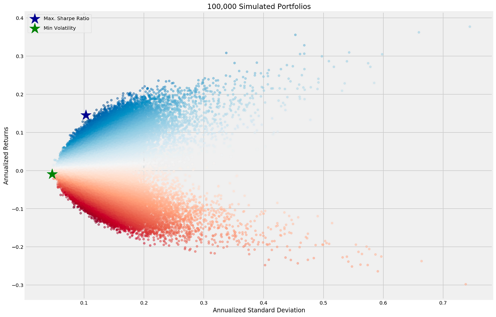
By analyzing the annualized returns and standard deviations of 100,000 simulated portfolios, the code snippet generates a scatter plot. An x-axis indicates portfolio risk, while a y-axis represents potential profit. The points represent different portfolios, with colors ranging from blue to red to indicate varying returns.
In the code, two key portfolios are highlighted: the portfolio with the highest Sharpe ratio, indicated by a dark blue star, and the one with the lowest volatility, indicated by a green star. An investor seeking to optimize their risk-return balance needs these portfolios.
With a gradient color scheme, the output plot emphasizes the risk-return relationship of simulated portfolios. Using the legend in the upper left corner, you can quickly identify the maximum Sharpe ratio and minimum volatility portfolio markers. In order to quickly evaluate portfolio selection trade-offs, the plot effectively conveys the results of the optimization process.
def portfolio_std(wt, rt=None, cov=None):
    """Annualized PF standard deviation"""
    return np.sqrt(wt @ cov @ wt * periods_per_year)
An annualized standard deviation, which measures risk, is calculated by using a vector of asset weights. Those parameters include returns, which are not used in this calculation, as well as a covariance matrix of asset returns, which measures the relationship between returns from different assets.
It computes portfolio variance by multiplying the weight vector with the covariance matrix, which generates a new vector based on the allocations between assets. Finalizing the variance calculation is done by multiplying the result by the weight vector again. By multiplying the variance by the period per year, we are able to adjust the standard deviation from the original period to a yearly perspective. As a result, the portfolio’s standard deviation indicates how much it could deviate from its average returns by taking the square root of this value. Based on asset allocation and return covariance, this function can be used to assess portfolio risk levels.
def portfolio_returns(wt, rt=None, cov=None):
    """Annualized PF returns"""
    return (wt @ rt + 1) ** periods_per_year - 1
An asset weight and its return are used to calculate annualized returns. Three parameters are required: weights representing the investment proportions for each asset, periodic returns for the assets, and a covariance parameter for future expansion.
By multiplying the weighted sum of returns by one, the matrix multiplication operator computes the growth factor by adding one. This function calculates the weighted sum of returns. A growth factor multiplied by the number of periods in a year annualizes returns, while subtracting one reduces it to a percentage. Scaled annualized returns can be calculated by providing the correct weights and returns. Adding error handling for missing values in the returns and covariance parameters will improve the code’s robustness.
def portfolio_performance(wt, rt, cov):
    """Annualized PF returns & standard deviation"""
    r = portfolio_returns(wt, rt=rt)
    sd = portfolio_std(wt, cov=cov)
    return r, sd
An annualized return and standard deviation for a financial portfolio are calculated by portfolio_performance. This function takes three arguments: wt, rt, and cov, which describe the covariance matrix of asset returns. By calling portfolio_returns function with weights and returns, it first calculates the overall portfolio return and stores the result in r. After calculating the portfolio’s standard deviation using the portfolio_std function with the same weights and covariance matrix, it stores this value in sd. It then returns a tuple that contains the portfolio’s annualized return and standard deviation.
def neg_sharpe_ratio(weights, mean_ret, cov):
    r, sd = portfolio_performance(weights, mean_ret, cov)
    return -(r - rf_rate) / sd
Neg_sharpe_ratio computes a negative Sharpe ratio for a set of portfolio weights, enabling optimization tasks to minimize risk. There are three parameters: weights, mean_ret, the expected returns, and cov, the covariance matrix of asset returns that indicates risk. On the basis of the parameters provided, the function invokes another function, portfolio_performance, to determine the expected return and standard deviation. Using the formula (r — rf_rate) / sd, it calculates a negative Sharpe ratio. To optimize investments, this inverted value helps determine their risk-adjusted performance.
weight_constraint = {'type': 'eq',
                     'fun': lambda x: np.sum(np.abs(x)) - 1}
An optimization problem requires the sum of the absolute values in an array to equal one as the weight constraint. A weight_constraint dictionary is defined in this code snippet. It is defined using a lambda function that takes an input x, which indicates that the constraint must be satisfied exactly rather than simply being less than or greater than a particular value. This function computes the absolute values of each element in x and subtracts one. In order for the constraint to be valid, it must return zero, ensuring the absolute values equal one. Keeping a specific scale is particularly useful for normalizing weights in optimization.
def max_sharpe_ratio(mean_ret, cov, short=True):
    return minimize(fun=neg_sharpe_ratio,
                    x0=x0,
                    args=(mean_ret, cov),
                    method='SLSQP',
                    bounds=((-1 if short else 0, 1),) * n_assets,
                    constraints=weight_constraint,
                    options={'tol':1e-10, 'maxiter':1e4})
The max_sharpe_ratio function optimizes the Sharpe ratio of a portfolio, which measures risk-adjusted return. The function takes mean_ret, representing the expected returns of the assets, and cov, the covariance matrix indicating the risk associated with asset returns, as inputs. The short parameter determines if short-selling is allowed; if set to True, the function accepts negative weights; if False, only non-negative weights are permitted.
The function employs the minimize function from the SciPy library to minimize an objective function called neg_sharpe_ratio, which calculates the negative of the Sharpe ratio to facilitate maximization. The x0 variable serves as the initial guess for asset weights. The arguments mean_ret and cov are passed to neg_sharpe_ratio during optimization. The optimization method used is the Sequential Least Squares Quadratic Programming algorithm, suitable for bounded constraint problems.
The bounds argument establishes limits for asset weights; allowed ranges vary from -1 to 1 for short-selling and from 0 to 1 when it is not permitted. Additionally, constraints are applied to the portfolio weights, ensuring compliance with specific conditions. The options parameter controls the tolerance level and maximum iterations for the optimization process, ensuring precision and preventing indefinite execution. Ultimately, this function aims to determine the optimal asset weights in a portfolio for maximizing the Sharpe ratio while accommodating short-selling if desired.
def min_vol_target(mean_ret, cov, target, short=True):

    def ret_(wt):
        return portfolio_returns(wt, mean_ret)

    constraints = [{'type': 'eq', 'fun': lambda x: ret_(x) - target},
                   weight_constraint]

    bounds = ((-1 if short else 0, 1),) * n_assets
    return minimize(portfolio_std,
                    x0=x0,
                    args=(mean_ret, cov),
                    method='SLSQP',
                    bounds=bounds,
                    constraints=constraints,
                    options={'tol': 1e-10, 'maxiter': 1e4})
The function min_vol_target minimizes portfolio volatility while achieving a specified target return. It takes four arguments: mean_ret, which represents expected asset returns; cov, the covariance matrix illustrating the movement of asset returns; target, the desired return; and short, a boolean indicating whether short selling is permitted.
Within the function, there is a nested function ret_ that calculates portfolio return based on asset weights. It utilizes an external function portfolio_returns to compute total returns based on the weights and mean returns. Constraints are established to ensure the solution meets the target return. The first constraint ensures the portfolio return equals the specified target, while the second, referred to as weight_constraint, maintains that the weights sum to a predefined value.
Bounds for asset weights are defined based on the short parameter. If short is true, weights can range down to -1, allowing shorting; if false, weights must be 0 or higher, prohibiting shorting. Each asset thus has identical bounds.
The function then calls minimize,from a library such as SciPy, to minimize portfolio volatility, using another function portfolio_std. Optimization starts with an initial guess for the weights and employs the Sequential Least Squares Programming method. Options are set for tight tolerance and a maximum number of iterations for improved accuracy.
This function systematically identifies the optimal asset distribution to meet the target return while minimizing risk.
def min_vol(mean_ret, cov, short=True):
    bounds = ((-1 if short else 0, 1),) * n_assets

    return minimize(fun=portfolio_std,
                    x0=x0,
                    args=(mean_ret, cov),
                    method='SLSQP',
                    bounds=bounds,
                    constraints=weight_constraint,
                    options={'tol': 1e-10, 'maxiter': 1e4})
The min_vol function identifies the minimum volatility portfolio based on expected returns, covariance, and short selling preferences. It begins by setting bounds for asset weights. If short selling is allowed, weights can range from -1 to 1. If not, weights are limited to 0 to 1, meaning all assets are held long. The bounds are applied for the number of assets in the portfolio.
Next, the function utilizes the minimize function from an optimization library, targeting the portfolio_std function, which calculates portfolio volatility based on the weights, mean returns, and covariance matrix. The optimization starts with an initial array of asset weights defined by x0. The function also accepts additional parameters like mean_ret and cov through the args parameter.
The optimization method employed is SLSQP, suitable for constrained problems. The bounds restrict asset weights according to short selling permissions, while a weight constraint ensures that the sum of weights equals 1, a common requirement. Finally, the optimization process is fine-tuned with options for tolerance and maximum iterations. This setup effectively determines the optimal asset allocation to minimize portfolio volatility based on the specified conditions.
def efficient_frontier(mean_ret, cov, ret_range, short=True):
    return [min_vol_target(mean_ret, cov, ret) for ret in ret_range]
The efficient_frontier function generates the efficient frontier for investment portfolios based on expected returns and the covariance of returns. It accepts three parameters: mean_ret, an array of expected returns for various assets; cov, the covariance matrix indicating how asset returns move together; and ret_range, a range of target returns for which minimum volatility needs to be determined. It also includes a short parameter, indicating whether short selling is allowed, set to true. The function uses a list comprehension to call min_vol_target for each target return in ret_range, calculating the minimum volatility portfolio for each. The resulting list shows the volatility associated with different expected return levels, which is essential for portfolio optimization.
simul_perf, simul_wt = simulate_portfolios(mean_returns, cov_matrix, short=True)This line of code calls the function simulate_portfolios, which generates portfolio simulations based on input parameters. The parameter mean_returns contains the average returns for different assets, representing the expected return for each asset. The cov_matrix is the covariance matrix that shows how returns on various assets move together, which is crucial for assessing risk in a portfolio. The function has a parameter named short set to True, indicating that the simulation allows for short-selling, enabling portfolios to include positions that bet on a decline in asset prices. The outputs simul_perf and simul_wt store performance information for each simulated portfolio, including returns or risk metrics, and the weights assigned to assets, respectively, detailing the allocation of each asset in the portfolios.
print(simul_perf.describe())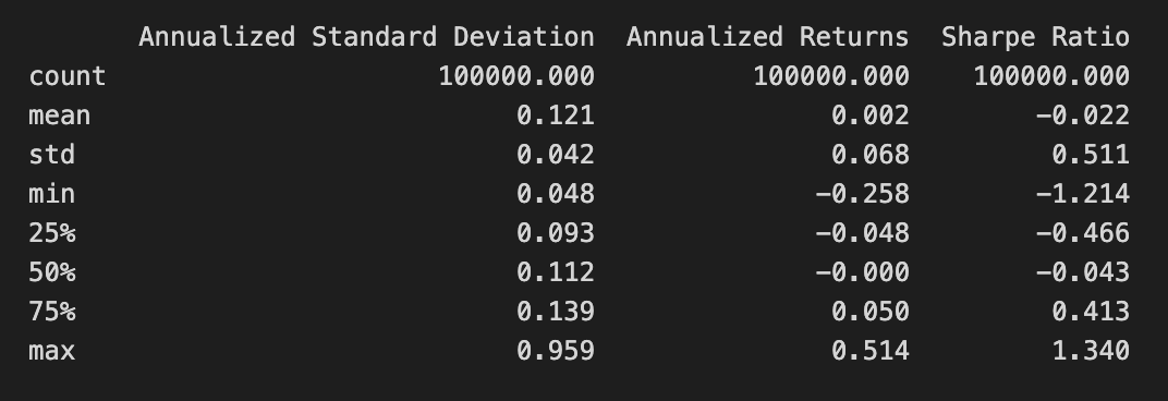
The code snippet print(simul_perf.describe()) generates a statistical summary of the simul_perf DataFrame, which contains performance metrics from a Mean-Variance Optimization project. It provides key statistics for three financial metrics: Annualized Standard Deviation, Annualized Returns, and Sharpe Ratio.
The Annualized Standard Deviation column reflects the volatility of returns, with a mean value of 0.121 indicating low average volatility. The maximum value of 0.959 shows instances of high volatility, while a standard deviation of 0.042 suggests slight variations around the mean. The minimum value of 0.048 indicates periods of very low volatility.
The Annualized Returns column shows the average returns from the investment strategy. The mean return is 0.002, signifying modest average returns. The maximum return of 0.514 indicates instances of significantly higher returns, while the minimum of -0.258 suggests some scenarios resulted in losses. The standard deviation of 0.068 reflects variability in returns during the simulation.
The Sharpe Ratio column measures risk-adjusted return, with a mean of -0.022 indicating that, on average, returns do not compensate for the risk taken. However, a maximum Sharpe Ratio of 1.340 suggests some scenarios significantly exceed the risk, while the minimum of -1.214 highlights poor performance instances.
This statistical summary offers a clear view of the investment strategy’s performance characteristics, aiding in the assessment of its risk and return profile, and informing decisions on portfolio optimization and risk management.
simul_max_sharpe = simul_perf.iloc[:, 2].idxmax()
simul_perf.iloc[simul_max_sharpe]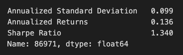
The code identifies the portfolio with the highest Sharpe ratio from a DataFrame named simul_perf. It retrieves the index of the maximum value from the third column, which represents the Sharpe ratios. The Sharpe ratio measures risk-adjusted return, indicating the excess return for the volatility of a riskier asset. Using the index, the code extracts the entire row corresponding to the portfolio with the highest Sharpe ratio, which includes essential performance metrics like annualized standard deviation, annualized returns, and the Sharpe ratio itself.
The output shows an annualized standard deviation of 0.099, reflecting the portfolio’s risk level, and annualized returns of 0.136, indicating the expected return over the year. The Sharpe ratio is 1.340, suggesting a favorable return compared to its risk, as a ratio above 1 is considered good. The output also confirms the index name and data type of the analyzed data. This code effectively identifies and presents the optimal portfolio based on the Sharpe ratio, supporting investment decision-making.
max_sharpe_pf = max_sharpe_ratio(mean_returns, cov_matrix, short=False)
max_sharpe_perf = portfolio_performance(max_sharpe_pf.x, mean_returns, cov_matrix)
This snippet focuses on optimizing a portfolio to achieve the maximum Sharpe ratio, which measures risk-adjusted return. The first line calls the max_sharpe_ratio function with mean_returns and cov_matrix as key arguments, where mean_returns indicates expected asset returns and cov_matrix conveys how asset returns interact. The short parameter is set to False, meaning short-selling is not permitted.
The second line takes the optimal asset allocation from the first line and uses it, along with mean_returns and cov_matrix, to call the portfolio_performance function. This function calculates various performance metrics, such as expected return, volatility, and the Sharpe ratio. Together, these lines determine the best asset allocation for maximizing risk-adjusted return and compute the performance metrics for that portfolio.
r, sd = max_sharpe_perf
pd.Series({'ret': r, 'sd': sd, 'sr': (r-rf_rate)/sd})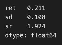
The code snippet extracts the maximum Sharpe ratio performance from a variable named max_sharpe_perf, which contains two values: return and standard deviation. A Pandas Series summarizes key performance metrics of a portfolio, showing a return of 0.211, or 21.1%, and a standard deviation of 0.108, indicating the portfolio’s risk with returns varying by about 10.8%. The Sharpe ratio is calculated using the formula (return — risk-free rate) / standard deviation, resulting in approximately 1.924. This suggests a favorable return per unit of risk, as a Sharpe ratio above 1 is generally seen as good. The Series is stored as float64, confirming the values are floating-point numbers, typical for financial metrics. This summary enables investors to assess the performance and risk profile of the portfolio in the context of mean-variance optimization.
min_vol_pf = min_vol(mean_returns, cov_matrix, short=False)
min_vol_perf = portfolio_performance(min_vol_pf.x, mean_returns, cov_matrix)
This code calculates the optimal minimal volatility portfolio using two functions: min_vol and portfolio_performance. The function min_vol takes expected returns and the covariance matrix of asset returns as inputs to determine the asset weights that minimize the portfolio’s volatility. The parameter short is set to false, which means short-selling is not allowed, ensuring all asset weights are non-negative. The output of this function is an array of weights indicating how to allocate assets for minimum volatility.
The next step involves the function portfolio_performance, which evaluates the performance metrics of the minimum volatility portfolio using the asset weights obtained from min_vol. This function typically returns values such as expected return, volatility, and possibly the Sharpe ratio, providing insights into the portfolio’s expected performance based on the input data.
def efficient_frontier(mean_ret, cov, ret_range, short=True):
    return [min_vol_target(mean_ret, cov, ret) for ret in ret_range]
The efficient_frontier function generates the efficient frontier for investment portfolios based on expected returns and the covariance of returns. It accepts three parameters: mean_ret, an array of expected returns for various assets; cov, the covariance matrix indicating how asset returns move together; and ret_range, a range of target returns for which minimum volatility needs to be determined. It also includes a short parameter, indicating whether short selling is allowed, set to true. The function uses a list comprehension to call min_vol_target for each target return in ret_range, calculating the minimum volatility portfolio for each. The resulting list shows the volatility associated with different expected return levels, which is essential for portfolio optimization.
simul_perf, simul_wt = simulate_portfolios(mean_returns, cov_matrix, short=True)This line of code calls the function simulate_portfolios, which generates portfolio simulations based on input parameters. The parameter mean_returns contains the average returns for different assets, representing the expected return for each asset. The cov_matrix is the covariance matrix that shows how returns on various assets move together, which is crucial for assessing risk in a portfolio. The function has a parameter named short set to True, indicating that the simulation allows for short-selling, enabling portfolios to include positions that bet on a decline in asset prices. The outputs simul_perf and simul_wt store performance information for each simulated portfolio, including returns or risk metrics, and the weights assigned to assets, respectively, detailing the allocation of each asset in the portfolios.
print(simul_perf.describe())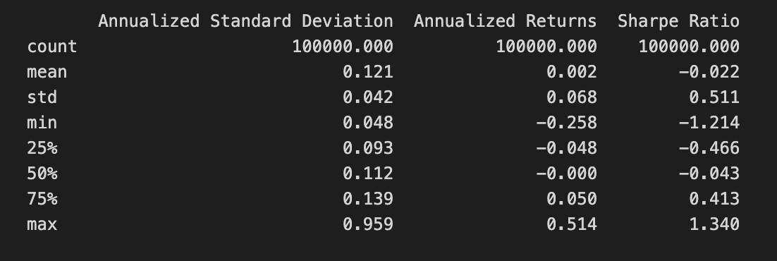
The code snippet print(simul_perf.describe()) generates a statistical summary of the simul_perf DataFrame, which contains performance metrics from a Mean-Variance Optimization project. It provides key statistics for three financial metrics: Annualized Standard Deviation, Annualized Returns, and Sharpe Ratio.
The Annualized Standard Deviation column reflects the volatility of returns, with a mean value of 0.121 indicating low average volatility. The maximum value of 0.959 shows instances of high volatility, while a standard deviation of 0.042 suggests slight variations around the mean. The minimum value of 0.048 indicates periods of very low volatility.
The Annualized Returns column shows the average returns from the investment strategy. The mean return is 0.002, signifying modest average returns. The maximum return of 0.514 indicates instances of significantly higher returns, while the minimum of -0.258 suggests some scenarios resulted in losses. The standard deviation of 0.068 reflects variability in returns during the simulation.
The Sharpe Ratio column measures risk-adjusted return, with a mean of -0.022 indicating that, on average, returns do not compensate for the risk taken. However, a maximum Sharpe Ratio of 1.340 suggests some scenarios significantly exceed the risk, while the minimum of -1.214 highlights poor performance instances.
This statistical summary offers a clear view of the investment strategy’s performance characteristics, aiding in the assessment of its risk and return profile, and informing decisions on portfolio optimization and risk management.
simul_max_sharpe = simul_perf.iloc[:, 2].idxmax()
simul_perf.iloc[simul_max_sharpe]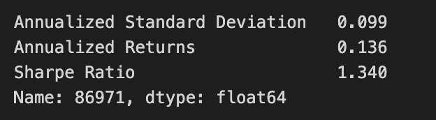
The code identifies the portfolio with the highest Sharpe ratio from a DataFrame named simul_perf. It retrieves the index of the maximum value from the third column, which represents the Sharpe ratios. The Sharpe ratio measures risk-adjusted return, indicating the excess return for the volatility of a riskier asset. Using the index, the code extracts the entire row corresponding to the portfolio with the highest Sharpe ratio, which includes essential performance metrics like annualized standard deviation, annualized returns, and the Sharpe ratio itself.
The output shows an annualized standard deviation of 0.099, reflecting the portfolio’s risk level, and annualized returns of 0.136, indicating the expected return over the year. The Sharpe ratio is 1.340, suggesting a favorable return compared to its risk, as a ratio above 1 is considered good. The output also confirms the index name and data type of the analyzed data. This code effectively identifies and presents the optimal portfolio based on the Sharpe ratio, supporting investment decision-making.
max_sharpe_pf = max_sharpe_ratio(mean_returns, cov_matrix, short=False)
max_sharpe_perf = portfolio_performance(max_sharpe_pf.x, mean_returns, cov_matrix)
This snippet focuses on optimizing a portfolio to achieve the maximum Sharpe ratio, which measures risk-adjusted return. The first line calls the max_sharpe_ratio function with mean_returns and cov_matrix as key arguments, where mean_returns indicates expected asset returns and cov_matrix conveys how asset returns interact. The short parameter is set to False, meaning short-selling is not permitted.
The second line takes the optimal asset allocation from the first line and uses it, along with mean_returns and cov_matrix, to call the portfolio_performance function. This function calculates various performance metrics, such as expected return, volatility, and the Sharpe ratio. Together, these lines determine the best asset allocation for maximizing risk-adjusted return and compute the performance metrics for that portfolio.
r, sd = max_sharpe_perf
pd.Series({'ret': r, 'sd': sd, 'sr': (r-rf_rate)/sd})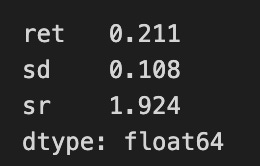
The code snippet extracts the maximum Sharpe ratio performance from a variable named max_sharpe_perf, which contains two values: return and standard deviation. A Pandas Series summarizes key performance metrics of a portfolio, showing a return of 0.211, or 21.1%, and a standard deviation of 0.108, indicating the portfolio’s risk with returns varying by about 10.8%. The Sharpe ratio is calculated using the formula (return — risk-free rate) / standard deviation, resulting in approximately 1.924. This suggests a favorable return per unit of risk, as a Sharpe ratio above 1 is generally seen as good. The Series is stored as float64, confirming the values are floating-point numbers, typical for financial metrics. This summary enables investors to assess the performance and risk profile of the portfolio in the context of mean-variance optimization.
min_vol_pf = min_vol(mean_returns, cov_matrix, short=False)
min_vol_perf = portfolio_performance(min_vol_pf.x, mean_returns, cov_matrix)
This code calculates the optimal minimal volatility portfolio using two functions: min_vol and portfolio_performance. The function min_vol takes expected returns and the covariance matrix of asset returns as inputs to determine the asset weights that minimize the portfolio’s volatility. The parameter short is set to false, which means short-selling is not allowed, ensuring all asset weights are non-negative. The output of this function is an array of weights indicating how to allocate assets for minimum volatility.
The next step involves the function portfolio_performance, which evaluates the performance metrics of the minimum volatility portfolio using the asset weights obtained from min_vol. This function typically returns values such as expected return, volatility, and possibly the Sharpe ratio, providing insights into the portfolio’s expected performance based on the input data.
ret_range = np.linspace(0, simul_perf.iloc[:, 1].max() * 1.1, 25)
eff_pf = efficient_frontier(mean_returns, cov_matrix, ret_range,short=False)
This code constructs an efficient frontier, which visually represents the relationship between risk and return for various portfolios. It begins by creating a return range using np.linspace, generating an array of 25 evenly spaced values from 0 to 10% above the maximum performance metric in the second column of the simul_perf DataFrame. This range serves as potential return targets for the portfolios. The return range is then passed to the efficient_frontier function, along with mean_returns and cov_matrix, which represent expected returns and the covariance matrix of different assets. The short=False argument indicates that short selling is not permitted in the portfolio construction. Overall, this code effectively establishes a set of target returns and calculates optimal asset allocations based on the provided statistical data.
fig, ax = plt.subplots()
simul_perf.plot.scatter(x=0, y=1, c=2, ax=ax,
                                 cmap='RdBu',
                                 alpha=0.5, figsize=(14, 9), colorbar=False,
                                 title='Mean-Variance Efficient Frontier')

r, sd = max_sharpe_perf
ax.scatter(sd, r, marker='*', color='r', s=500, label='Max Sharpe Ratio PF')

r, sd = min_vol_perf
ax.scatter(sd, r, marker='*', color='g', s=500, label='Min Volatility PF')

kelly_wt = precision_matrix.dot(mean_returns).values
kelly_wt /= np.sum(np.abs(kelly_wt))
r, sd = portfolio_performance(kelly_wt, mean_returns, cov_matrix)
ax.scatter(sd, r, marker='*', color='darkgrey', s=500, label='Kelly PF')

std = monthly_returns.std()
std /= std.sum()
r, sd = portfolio_performance(std, mean_returns, cov_matrix)
ax.scatter(sd, r, marker='*', color='y', s=500, label='Risk Parity PF')

r, sd = portfolio_performance(np.full(n_assets, 1/n_assets), mean_returns, cov_matrix)
ax.scatter(sd, r, marker='*', color='blue', s=500, label='1/n PF')

ax.plot([p['fun'] for p in eff_pf], ret_range,
        linestyle='--', lw=3, color='darkgrey', label='Efficient Frontier')
ax.legend(labelspacing=0.8)
fig.tight_layout();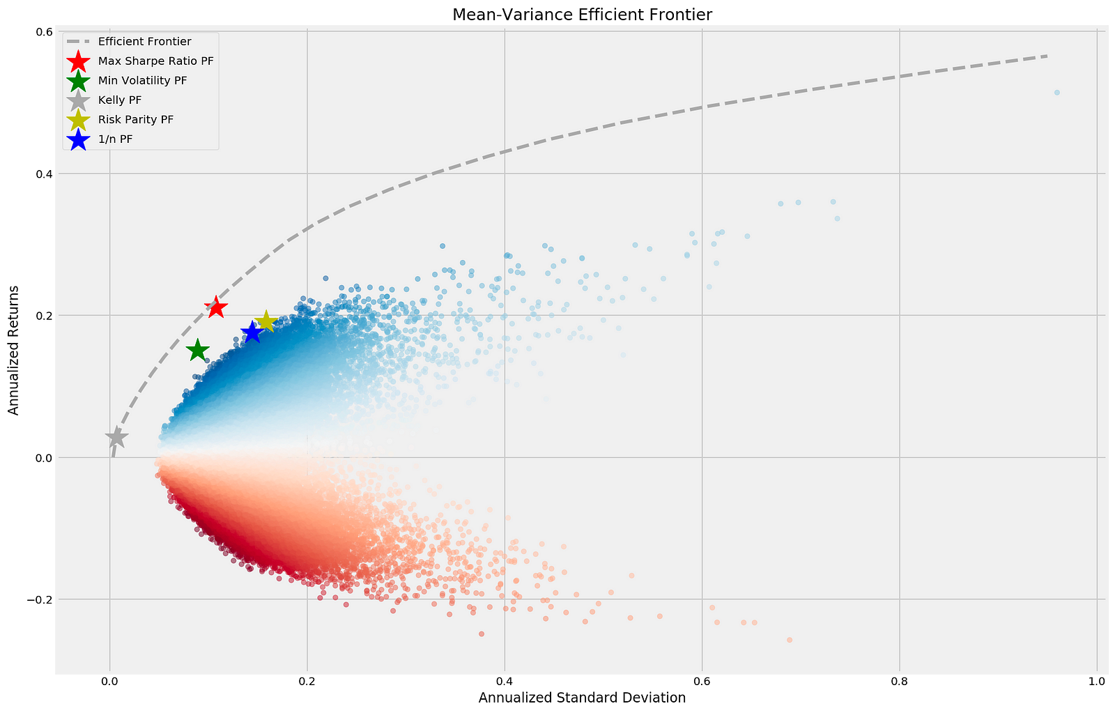
The code generates a scatter plot that visualizes the Mean-Variance Efficient Frontier, an essential concept in portfolio optimization. Using Matplotlib, it depicts the annualized standard deviation (risk) on the x-axis and annualized returns on the y-axis for various portfolios. The scatter plot is based on the simul_perf DataFrame, with colors indicating the performance of different portfolios and adjusted transparency using the alpha parameter. The title of the plot is Mean-Variance Efficient Frontier.
Key portfolios are highlighted: the maximum Sharpe ratio portfolio is marked with a red star, representing the best return per unit of risk, while the minimum volatility portfolio is indicated by a green star, reflecting the lowest risk. The Kelly portfolio is shown in dark grey, the risk parity portfolio in yellow, and the equal-weight portfolio in blue, which allocates equal weights to all assets. The efficient frontier is represented by a dashed line, signifying the optimal portfolios that provide the highest expected return for a given level of risk, typically sloping upward to show the relationship between risk and return. The legend clarifies the different portfolios and their markers. This output effectively demonstrates the risk-return relationship for various investment strategies, facilitating the comparative analysis of portfolio performance in mean-variance optimization.
std = monthly_returns.std()
std /= std.sum()
r, sd = portfolio_performance(std, mean_returns, cov_matrix)
r, sd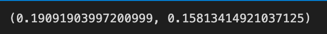
The code calculates the standard deviation of monthly returns and normalizes it by dividing each standard deviation by the total sum of standard deviations. This normalization ensures that the weights of the assets in the portfolio equal one, which is crucial for portfolio optimization. The portfolio_performance function is then invoked with the normalized standard deviations, mean returns, and the covariance matrix of the assets to compute the expected return and risk of the portfolio.
The output is a tuple containing two values: the expected return of the portfolio, approximately 0.1909, and the portfolio’s risk, represented by a standard deviation of about 0.1581. These results highlight the trade-off between risk and return in mean-variance optimization, aiming to maximize returns for a given risk level or minimize risk for a specific return. The values indicate a portfolio expected to yield a return of about 19.09% with a risk level of 15.81%, aiding investors in making informed decisions based on their risk tolerance and investment objectives.
Kelly Rule
%matplotlib inline
from sympy import symbols, solve, log, diff
from scipy.optimize import minimize_scalar, newton, minimize
from scipy.integrate import quad
from scipy.stats import norm
import numpy as np
import pandas as pd
from numpy.linalg import inv
import matplotlib.pyplot as plt
from numpy.random import dirichlet
import warnings
This snippet sets up the environment for scientific computation and plotting in Python, specifically for use in Jupyter notebooks where plots are displayed inline. It imports several libraries essential for various mathematical tasks. SymPy is included for symbolic mathematics, allowing the definition of variables, equation solving, logarithm computation, and derivative calculation. SciPy is imported for numerical computations, providing functions for optimization and integration, as well as dealing with normal distributions. NumPy is essential for handling arrays and numerical operations, including random sampling. Pandas is used for data manipulation and analysis, particularly with structured data. Matplotlib is included for creating visualizations. The inv function from NumPy’s linear algebra module is necessary for computing matrix inverses. The warnings module is also imported to manage any warning messages during execution. This setup facilitates complex mathematical operations, statistical analysis, and visualizations, with each library serving a specific purpose for the computations that will follow.
warnings.filterwarnings('ignore')
plt.style.use('fivethirtyeight')
np.random.seed(42)
This snippet establishes the environment for data visualization and random number generation in Python. It begins by using the command to suppress any warning messages during code execution, which helps maintain a clean output during exploratory analysis or when warnings are deemed irrelevant. The snippet then applies a specific aesthetic style to Matplotlib plots, enhancing their visual appeal by mimicking the design of the FiveThirtyEight website. Finally, it sets a fixed seed for NumPy’s random number generation, ensuring reproducibility of results. By using the same seed, you guarantee that every execution of the code yields the same sequence of random numbers, aiding in debugging and facilitating result replication by others.
share, odds, probability = symbols('share odds probability')
Value = probability * log(1 + odds * share) + (1 - probability) * log(1 - share)
solve(diff(Value, share), share)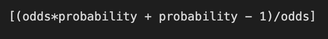
The code snippet employs symbolic mathematics to derive a formula for the Kelly Criterion, a strategy used for determining bet sizes in gambling and investing. It defines three symbols: share, odds, and probability. The variable Value calculates the expected logarithmic utility of a bet based on these three symbols.
Value is constructed using the logarithm function, which is integral to utility theory. It considers two outcomes: winning the bet, represented by the term probability times log(1 plus odds times share), and losing the bet, represented by (1 minus probability) times log(1 minus share). This formulation reflects the balance between potential gains and losses from the bet.
Next, the code differentiates Value with respect to share to identify the optimal bet size that maximizes expected utility. The solve function determines the value of share that yields a stationary point of the utility function, indicating a potential maximum or minimum.
The code outputs a symbolic expression for the optimal bet size based on the odds and probability. It reveals that the optimal share to bet is given by the formula (odds times probability plus probability minus 1) divided by odds. This demonstrates how the optimal bet size changes with fluctuations in odds and the probability of winning, in line with the principles of the Kelly Criterion.
f, p = symbols('f p')
y = p * log(1 + f) + (1 - p) * log(1 - f)
solve(diff(y, f), f)
The code defines a mathematical expression related to the Kelly Criterion, used to determine the optimal size of bets in gambling or investment. It imports symbolic computation tools and defines two symbols, f representing the fraction of the bankroll to bet and p representing the probability of winning.
The expression y combines logarithmic functions: the first term, p multiplied by the logarithm of 1 plus f, shows the expected logarithmic return when winning, while the second term, (1 minus p) multiplied by the logarithm of 1 minus f, represents the expected return when losing. This formulation highlights the balance between risk and reward, emphasizing the significance of both winning probability and the fraction of the bankroll involved.
The code differentiates the expression y with respect to f to identify critical points crucial for finding the optimal betting fraction. The solve function determines the values of f that maximize the expected logarithmic return. The output indicates that the optimal fraction to bet is 2p minus 1, showing a direct relationship with the probability of winning. If p exceeds 0.5, the optimal bet size increases, suggesting that a larger fraction of the bankroll should be bet when the probability of winning is favorable. In contrast, if p is below 0.5, the output advises against placing bets, as the expected return would be negative.
This analysis offers clear guidance for bettors or investors on sizing bets based on perceived success probabilities, aligning with the Kelly Criterion principles. The output succinctly encapsulates the link between winning probability and the optimal betting strategy, reinforcing that informed decision-making leads to better long-term outcomes.
with pd.HDFStore('../../data/assets.h5') as store:
    sp500 = store['sp500/prices'].close
This snippet utilizes the pandas library to handle HDF5 files, which are intended for storing large datasets. It employs pd.HDFStore as a context manager to open the HDF5 file at ../../data/assets.h5. Within the with block, it accesses the dataset located at sp500/prices and retrieves the close column, which contains the closing prices of the S&P 500 index. Once the with block is exited, the HDFStore is automatically closed, ensuring proper resource management. This approach simplifies access to the closing prices without manual file loading and unloading.
annual_returns = sp500.resample('A').last().pct_change().to_frame('sp500')This code calculates the annual returns of the S&P 500 index by resampling the data to annual frequency, selecting the last observation of each year. It then computes the percentage change between the last value of each year and the previous year, which results in the annual return as a percentage. Finally, it converts the series of percentage changes into a DataFrame, naming the column sp500. The variable annual_returns thus contains a DataFrame with the annual returns of the S&P 500, allowing for straightforward year-over-year performance analysis.
return_params = annual_returns.sp500.rolling(25).agg(['mean', 'std']).dropna()This line of code processes annual returns for the S&P 500, stored in a DataFrame or Series named annual_returns.sp500. It computes a rolling window of 25 periods, analyzing the last 25 annual returns for each point in the series. The agg method, with parameters mean and std, calculates the average and standard deviation for each 25-period window. The dropna method removes rows with missing values, ensuring that the result includes only valid calculations where there are enough data points. The final output is a DataFrame that presents the rolling mean and standard deviation of the S&P 500 annual returns over 25 years, with each row corresponding to a valid point in time.
return_ci = (return_params[['mean']]
                .assign(lower=return_params['mean'].sub(return_params['std'].mul(2)))
                .assign(upper=return_params['mean'].add(return_params['std'].mul(2))))
This code snippet calculates a confidence interval for a set of return parameters using a DataFrame named return_params, which has a column labeled mean. A new DataFrame, return_ci, is created to include these mean values along with their corresponding lower and upper confidence bounds.
The process starts by selecting the mean column from return_params. It then uses the assign method to add two new columns: lower and upper. The lower bound is calculated by subtracting twice the standard deviation from the mean, and the upper bound is obtained by adding twice the standard deviation to the mean. This approach, which assumes a normal distribution of the data, defines the bounds of a confidence interval. As a result, the return_ci DataFrame will consist of the mean, lower confidence limit, and upper confidence limit for the return parameters.
return_ci.plot(lw=2, figsize=(14, 8));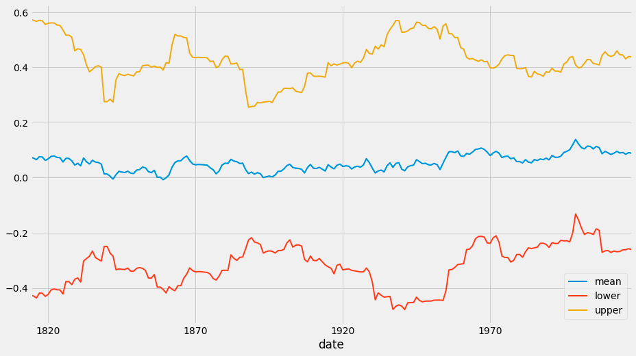
The code snippet return_ci.plot(lw=2, figsize=(14, 8)) creates a visual representation of a dataset related to the Kelly Criterion, which determines the optimal size of bets in gambling or investing. The return_ci variable contains a DataFrame with statistical data, including mean returns and confidence intervals over time. The output displays three lines plotted against a timeline from the early 1800s to the late 1970s. The blue line indicates the mean return, the red line represents the lower confidence interval, and the orange line represents the upper confidence interval. These intervals show the range within which the true mean return is expected to lie, offering insights into the volatility and reliability of the returns. The visualization reveals trends in mean return over time, with fluctuations suggesting varying performance periods. The confidence intervals help indicate uncertainty, with wider intervals reflecting greater variability in returns. Analyzing the relationship between the mean and confidence intervals provides a better understanding of the investment strategy’s risk and the potential for higher returns in specific periods. Overall, this plot effectively analyzes the Kelly Criterion’s effectiveness in sizing bets based on historical data.
def norm_integral(f, mean, std):
    val, er = quad(lambda s: np.log(1 + f * s) * norm.pdf(s, mean, std),
                               mean - 3 * std,
                               mean + 3 * std)
    return -val
The norm_integral function calculates an integral involving a function f, a mean, and a standard deviation. It utilizes the quad function from the scipy.integrate module for numerical integration. The integral evaluates a lambda function combining np.log(1 + f * s) and norm.pdf(s, mean, std). Here, np.log(1 + f * s) computes the natural logarithm of 1 plus the product of f and s, while norm.pdf(s, mean, std) represents the probability density function of a normal distribution, providing weights for each point s based on the normal distribution’s likelihood. The integration limits are set from mean minus three times the standard deviation to mean plus three times the standard deviation, encompassing approximately 99.7% of the distribution area. The integral value is returned with a negative sign, which may indicate a negative logarithm or a transformation that occurs after integration, depending on the intended use of the result.
def norm_dev_integral(f, mean, std):
    val, er = quad(lambda s: (s / (1 + f * s)) * norm.pdf(s, mean, std), m-3*std, mean+3*std)
    return val
The norm_dev_integral function computes a specific integral based on the parameters provided. It takes three arguments: f, mean, and std, where f is a coefficient influencing the integral, and mean and std are the mean and standard deviation of a normal distribution. The function utilizes the quad method from SciPy for numerical integration, performed over the range from mean — 3 * std to mean + 3 * std, which captures about 99.7% of the area under the normal curve according to the empirical rule. The integrand is a lambda function that calculates the expression (s / (1 + f * s)) * norm.pdf(s, mean, std), where norm.pdf(s, mean, std) represents the probability density function of the normal distribution at point s with the specified parameters. The function ultimately returns the value of the integral computed by quad. An error estimate is generated but is not utilized. This integral is applicable in various fields, particularly in statistics and probability analysis involving normal distribution modeling.
def get_kelly_share(data):
    solution = minimize_scalar(norm_integral,
                        args=(data['mean'], data['std']),
                        bounds=[0, 2],
                        method='bounded')
    return solution.x
The function get_kelly_share calculates the Kelly criterion to determine the optimal bet size for a betting strategy based on expected returns. It accepts a data dictionary containing the mean and standard deviation of returns. The function uses minimize_scalar from an optimization library, SciPy, to find the optimal value.
