


Optimizing Trading Strategies with Machine Learning: A Practical Guide
Optimizing Trading Strategies with Machine Learning: A Practical Guide
Leveraging SMA, SVM, and AdaBoost for Enhanced Market Returns

Welcome to the intricate world of algorithmic trading, where the confluence of data analysis and machine learning can unlock new strategies for market success. This article delves into the application of sophisticated machine learning techniques to optimize trading algorithms. We begin by setting up our coding environment, importing essential libraries like Pandas, Numpy, and SKLearn, vital for data manipulation, statistical operations, and machine learning model implementation.
Download the source code from the link in the comment section.
The journey starts with establishing a baseline performance for a trading algorithm, where we systematically import and preprocess financial data, specifically OHLCV datasets. By applying simple moving averages (SMA) and generating trading signals, we create a foundational model for market analysis. The article then shifts gears towards more advanced techniques, introducing machine learning models such as Support Vector Machines (SVM) and AdaBoost Classifiers. These models are meticulously trained and tested against our trading data, with a keen focus on tuning parameters to enhance performance.
Each step of the process is accompanied by detailed code snippets and explanations, ensuring a comprehensive understanding of how each component contributes to the overall strategy. From data preprocessing, feature engineering to model evaluation and backtesting, the article is a step-by-step guide to refining a trading algorithm for improved strategy returns.
In the culmination of our efforts, we compare the performance of these models, visualizing their effectiveness through cumulative return plots and classification reports. This practical approach not only illustrates the power of machine learning in financial strategies but also serves as a blueprint for traders and analysts keen on integrating these technologies into their market analysis toolkit.
# Imports
import pandas as pd
import numpy as np
from pathlib import Path
import hvplot.pandas
import matplotlib.pyplot as plt
from sklearn import svm
from sklearn import metrics
from sklearn.ensemble import AdaBoostClassifier
from sklearn.preprocessing import StandardScaler
from pandas.tseries.offsets import DateOffset
from sklearn.metrics import classification_report
This code imports several libraries including pandas, numpy, and matplotlib.pyplot that provide helpful functions and tools for analyzing and visualizing data. It also imports machine learning tools such as svm, metrics, AdaBoostClassifier, and StandardScaler that can be used for building and evaluating predictive models. Additionally, the code imports DateOffset from pandas.tseries.offsets, which allows for performing date calculations and incorporating date information into data analysis. Lastly, the code imports classification_report from sklearn.metrics, which is used for obtaining detailed information on the performance of a classification model. Overall, this code sets up the environment and tools necessary for performing data analysis and building machine learning models.
Establishing a Baseline Performance
This section is dedicated to establishing a baseline performance for the trading algorithm. To accomplish this, you will need to complete a series of steps:
Start by opening the Jupyter notebook provided. Once it’s open, proceed by restarting the kernel to ensure that you are working in a clean environment. Next, run the cells in the notebook that correspond to the first three steps as outlined in the starter code. After you have completed these initial steps, move forward to step four.
These actions will help in setting a baseline performance for the trading algorithm, which is a crucial foundation for any further analysis and enhancements.
Step 1: mport the OHLCV dataset into a Pandas DataFrame.
# Import the OHLCV dataset into a Pandas Dataframe
ohlcv_df = pd.read_csv(
    Path("./Resources/emerging_markets_ohlcv.csv"),
    index_col='date',
    infer_datetime_format=True,
    parse_dates=True
)

# Review the DataFrame
ohlcv_df.head()
This code starts by importing the OHLCV Open-High-Low-Close-Volume dataset into a Pandas Dataframe called ohlcv_df. The dataset is being read in from the file emerging_markets_ohlcv.csv and is being assigned to the variable ohlcv_df. The index column of the Dataframe is set to date, which is the date of the market data. The time format of the dates in the dataset is being inferred and the dates are also being parsed. This allows for easier manipulation and analysis of the data in the Dataframe. Finally, the code prints the first few rows of the Dataframe to review and confirm that it has been successfully imported.
# Filter the date index and close columns
signals_df = ohlcv_df.loc[:, ["close"]]

# Use the pct_change function to generate  returns from close prices
signals_df["Actual Returns"] = signals_df["close"].pct_change()

# Drop all NaN values from the DataFrame
signals_df = signals_df.dropna()

# Review the DataFrame
display(signals_df.head())
display(signals_df.tail())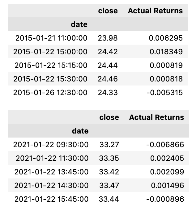
This code is used to filter a dataset by selecting only two columns — the date index and the close price — and storing them in a variable called signals_df. Then, the code uses the pct_change function to calculate the percentage change in the close prices over a certain period of time and adds it as a new column called Actual Returns in the signals_df dataframe. Next, the code drops all rows with missing values, as the pct_change function will return NaN Not a Number for the first row. The head and tail functions are then used to display the first and last five rows of the filtered dataset, respectively. This code snippet is often used in financial analysis to calculate and visualize the returns of a particular asset over a period of time.
Step 2: Generate trading signals using short- and long-window SMA values.
# Set the short window and long window
short_window = 4
long_window = 100

# Generate the fast and slow simple moving averages (4 and 100 days, respectively)
signals_df['SMA_Fast'] = signals_df['close'].rolling(window=short_window).mean()
signals_df['SMA_Slow'] = signals_df['close'].rolling(window=long_window).mean()

signals_df = signals_df.dropna()

# Review the DataFrame
display(signals_df.head())
display(signals_df.tail())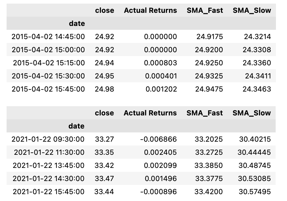
This code sets two variables, short_window and long_window, with values of 4 and 100 respectively. These represent the number of days used to calculate two types of simple moving averages SMA for a given stock, represented by a DataFrame called signals_df. The first SMA, called SMA_Fast, is calculated using the close column of the DataFrame and a rolling window of 4 days. The second SMA, called SMA_Slow, uses the same close column but with a longer window of 100 days. The DataFrame is then updated, dropping any rows with missing values, and the first and last few rows are displayed for review. Overall, this code is used to calculate and display two different types of moving averages for a given stock, with the number of days used for each being adjusted based on the values of the short_window and long_window variables.
# Initialize the new Signal column
signals_df['Signal'] = 0.0

# When Actual Returns are greater than or equal to 0, generate signal to buy stock long
signals_df.loc[(signals_df['Actual Returns'] >= 0), 'Signal'] = 1

# When Actual Returns are less than 0, generate signal to sell stock short
signals_df.loc[(signals_df['Actual Returns'] < 0), 'Signal'] = -1

# Review the DataFrame
display(signals_df.head())
display(signals_df.tail())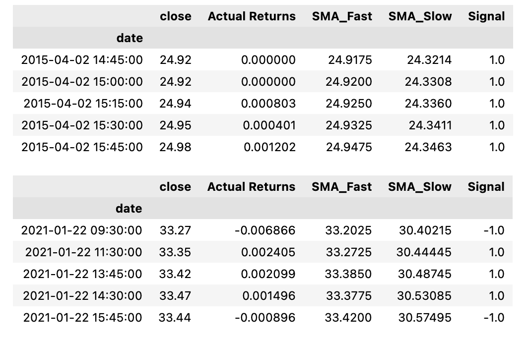
This code creates a new column in the dataframe called Signal and sets all values in that column to 0.0. Then, using conditional statements, it checks the values in the Actual Returns column. If the value is greater than or equal to 0, it changes the corresponding value in the Signal column to 1, indicating a signal to buy the stock. If the value is less than 0, it changes the corresponding value in the Signal column to -1, indicating a signal to sell the stock short. Finally, the code displays the first and last few rows of the updated dataframe with the new Signal column. In summary, this code generates buy and sell signals based on the values in the Actual Returns column and updates the dataframe with this information.
signals_df['Signal'].value_counts()
This code uses the value_counts function to count the number of occurrences of each unique value in the Signal column of the dataframe called signals_df. It then displays the result, showing the number of times each value appears. This is useful for understanding the distribution of data in the Signal column, and can help to identify any patterns or outliers.
# Calculate the strategy returns and add them to the signals_df DataFrame
signals_df['Strategy Returns'] = signals_df['Actual Returns'] * signals_df['Signal'].shift()

# Review the DataFrame
display(signals_df.head())
display(signals_df.tail())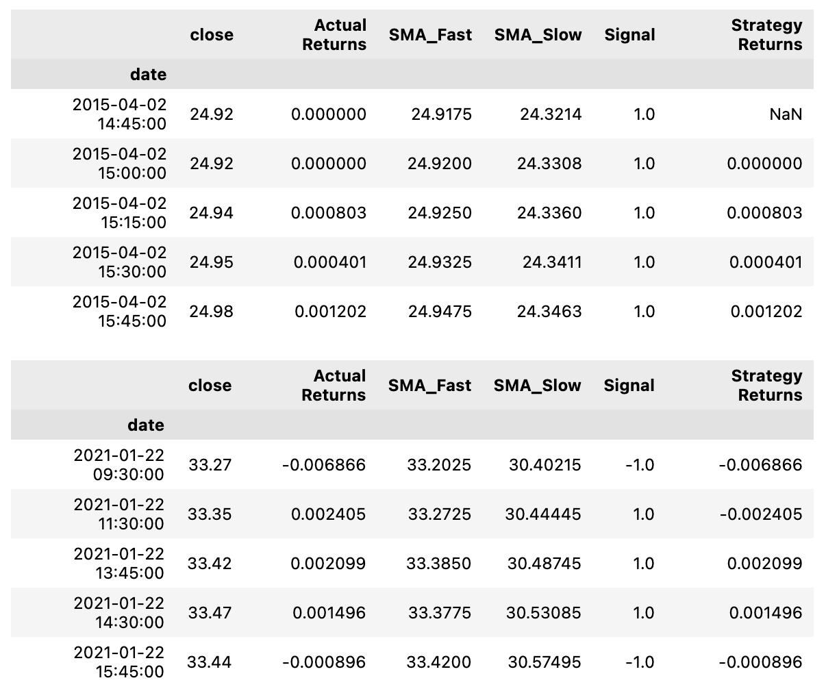
This code calculates the strategy returns and adds them to the signals_df DataFrame. The calculation is performed by multiplying the Actual Returns column with the Signal column, which has been shifted by one row. This takes into account the signal from the previous day to determine the strategy returns for the current day. The result is then added as a new column called Strategy Returns in the signals_df DataFrame. By doing this, the code is able to compare the returns of the strategy with the actual returns and assess the effectiveness of the chosen strategy. Finally, the code displays the first and last few rows of the updated DataFrame for review.
# Plot Strategy Returns to examine performance
(1 + signals_df['Strategy Returns']).cumprod().plot()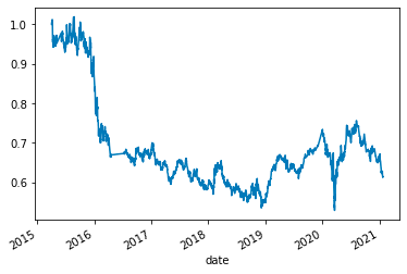
This code is meant to plot the strategy returns of an investment strategy. It uses the cumprod method to create a cumulative product of the strategy returns, which is plotted using the plot method. The strategy returns are calculated by adding 1 to the strategy returns data frame and multiplying it by the cumulative product, which represents the overall performance of the strategy. The resulting plot provides a visual representation of how the strategy has performed over time, allowing for an analysis of its effectiveness.