

Overview of Deep Learning using PyTorch
Deep learning enables computers and machines to perform cognitive tasks in real life by utilizing a class of machine learning methods.

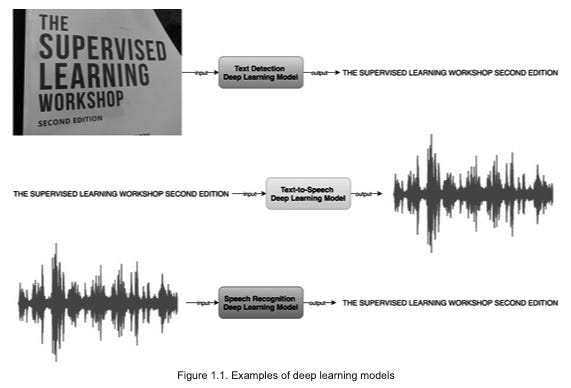
The concept of deep learning is based on the mathematical concept of deep neural networks. Deep learning learns nonlinear relationships between inputs and outputs using large amounts of data. Figure 1 illustrates some examples of inputs and outputs. They include:
Text image as input; text as output
The text is entered; the voice speaks it
A natural voice speaks the text; a transcription is created
The list goes on. To illustrate the preceding explanation, here is a figure:
In deep neural networks, a lot of math is involved, along with linear algebraic equations, nonlinear functions of complex complexity, and optimization algorithms. Using Python, we would have to write all the equations, functions, and optimization schedules necessary to build and train a deep neural network from scratch. It would also be necessary to write the code so that large amounts of data can be loaded efficiently and training can be done quickly. As a result, deep learning applications require several lower-level details to be implemented.
A number of deep learning libraries have been developed over the years to abstract away these details, including Theano and TensorFlow. To create deep learning models, Python-based PyTorch is one of the best options.
Applied deep learning has been revolutionized since Google introduced TensorFlow’s open source Python (and C++) library in late 2015. A deep learning library called Torch was developed by Facebook in 2016 as a response to this. As Torch evolved, a Python equivalent emerged called PyTorch, a scripting language based on Lua. CNTK, Microsoft’s own library, was also released at the same time. Since PyTorch became one of the most widely used deep learning libraries in the midst of hot competition, it has been growing rapidly.
In this book, you will learn how to use PyTorch to build, train, and evaluate some of the most advanced deep learning models. This book covers some of the most advanced deep learning problems as well as how to solve them using complex deep learning architectures.
As well as covering some of the most recent and advanced deep learning models, the book also covers PyTorch at the center of the discussion. Ideally, the reader should have experience with PyTorch and a working knowledge of Python.
In order to become proficient in writing PyTorch code, it is strongly advised that you try the examples in each chapter on your computer on your own. This introductory chapter will introduce the various features PyTorch offers, then we will go on to explore various deep-learning problems and model architectures.
The purpose of this chapter is to provide a brief overview of PyTorch and some of the concepts behind deep learning. Using PyTorch, we train a deep learning model at the end of this chapter.
This chapter will cover the following topics:
Deep learning refresher
Getting to know PyTorch
PyTorch is used to train neural networks
The technical requirements
For all of our exercises, we’ll use Jupyter notebooks. This chapter requires installing the following Python libraries with pip. To install torch==1.4.0, run pip install torch==1.4.0:
jupyter==1.0.0
torch==1.4.0
torchvision==0.5.0
matplotlib==3.1.2
A refresher on deep learning
The human brain’s structure and function inspire neural networks, one of the subtypes of machine learning methods. A neural network is composed of layers of computational units, analogously known as neurons. An artificial neural network formed by more than two layers is referred to as a deep neural network. This type of model is commonly referred to as a deep learning model.
Due to their ability to learn highly complex relationships between input data and output (ground truth), deep learning models have proven superior to other classical machine learning models. A lot of attention has been paid to deep learning recently, and rightly so. There are two main reasons for this:
Powerful computing machines, especially in the cloud, are readily available
There is a huge amount of data available
With Moore’s law, which states that computers’ processing power doubles every two years, it is now possible to train deep learning models with several hundreds of layers within an acceptable timeframe. Our digital footprint has expanded exponentially as the use of digital devices has grown everywhere, resulting in enormous amounts of data being generated every minute around the globe.
By using deep learning, it has become possible to train models to solve some of the most difficult cognitive tasks previously intractable or with suboptimal solutions.
A further advantage of deep learning is that it is more efficient than classical machine learning models. Feature engineering plays an important role in the overall performance of a trained model in a classical machine learning approach. It is, however, not necessary to manually craft features when using a deep learning model. Deep learning models are capable of outperforming traditional machine learning models when dealing with large amounts of data without requiring hand-engineered features. A comparison of deep learning models and classical machine learning models is shown in the following graph:

Up to a certain dataset size, deep learning performance doesn’t necessarily differ. In spite of this, deep neural networks begin to outperform non-deep learning models as the size of the data increases.
Different types of neural network architectures have been developed over the years that can be used to build deep learning models. Different neural networks use different types and combinations of layers, which is what distinguishes them. There are a number of well-known layers, including:
Fully-connected or linear: According to the following diagram, all neurons preceding and succeeding a fully connected layer are connected:
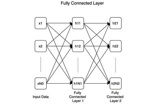
There are two consecutive layers with N1 and N2 number of neurons, respectively, in this example. Many — if not most — deep learning classifiers are built on fully connected layers.
Convolutional. A convolutional layer is shown in the following diagram, where convolutional kernels (or filters) are convolved over inputs:

Computer vision problems are best solved using convolutional neural networks (CNNs), which have convolutional layers as fundamental unit.
Recurrent. A recurrent layer is shown in the following diagram. Recurrent connections (marked with bold curved arrows) distinguish it from a fully connected layer.
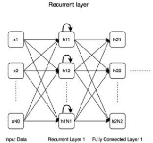
As opposed to fully connected layers, recurrent layers exhibit memorizing capabilities, which is handy when dealing with sequential data and needing to remember past inputs as well as current ones.
In the following diagram, a deconvolutional layer works in the exact opposite way of a convolutional layer:

Models that are aimed at generating or reconstructing images, for instance, require this layer to expand the input data spatially.
Pooling. A max-pooling layer, which is perhaps the most widely used type of pooling layer, can be seen in the following diagram:
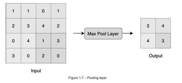
Using 2x2 sized subsections for the input, this layer pools the highest number from each subsection. There are two other types of pooling: min-pooling and mean-pooling.
Dropout: Dropout layers are illustrated in the following diagram. The dropout layer involves switching off some neurons (marked with an X in the diagram), i.e., disconnecting them from the network:
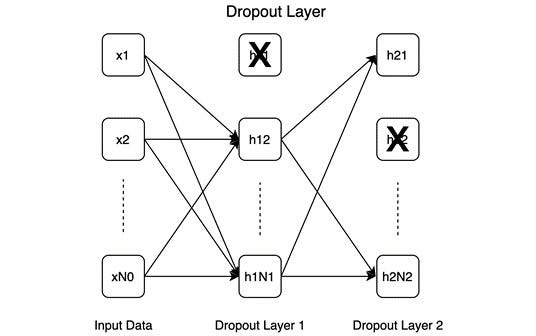
Model regularization is helped by dropout by forcing the model to function well when some neurons disappear, forcing the model to learn generalizable patterns rather than memorizing everything it learned during training.
The following diagram illustrates several well-known architectures based on the previously mentioned layers:.
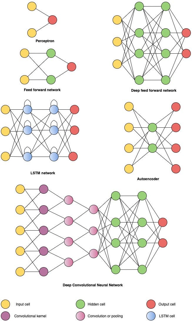
A more exhaustive set of neural network architectures can be found here: https://www.asimovinstitute.org/neural-network-zoo/.
An optimization schedule, activation functions, and activation functions are some of the other factors which define a model besides the types of layers.
Activation functions
Neural networks are non-linear without activation functions, which, no matter how many layers we add, would be reduced to linear models no matter how many layers we add. Here are a variety of different types of nonlinear mathematical activation functions.
The following are some of the most popular activation functions:
Sigmoid: An expression for a sigmoid (or logistic) function is as follows:

In graph form, the function looks like this:

In the graph, we can see that the sigmoid function takes an input value x and outputs a value y in the range (0, 1).
TanH: The expression for TanH is:

In graph form, the function looks like this:
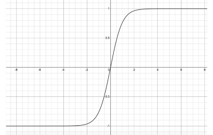
In contrast to sigmoid, TanH activation function output y is between -1 and 1. As a result, this activation can be used in cases where both positive and negative outputs are needed.
Rectified linear units (ReLUs): There are three types of ReLUs, the most recent two being:

In graph form, the function looks like this:
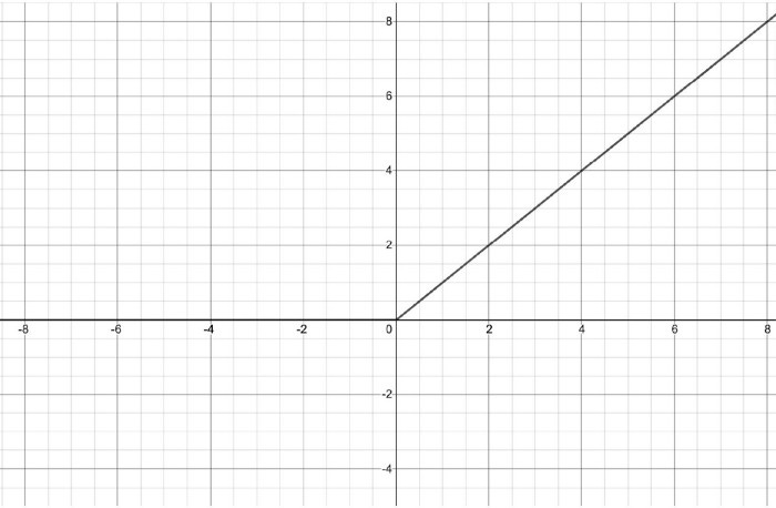
When the input is greater than 0, ReLU’s output keeps growing with the input, unlike the sigmoid and TanH activation functions. Unlike the previous two activation functions, the gradient of this function does not diminish to zero. In any case, both the output and gradient will be zero when the input is negative
A leaky ReLU outputs 0 in response to any incoming negative input: It is possible, however, that we will want to also process negative inputs in some cases. Negative inputs can be processed by leaky ReLUs by outputting a fraction k of the negative input. Activation function k has the following mathematical expression:
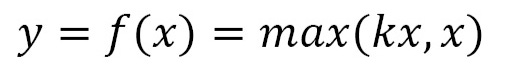
Here is a graph showing the input-output relationship for leaky ReLUs:
The field of activation functions is one of the most actively researched areas within deep learning. There are a number of activation functions that cannot be listed here, but I encourage you to look at the latest developments in this area. The activation functions described in this section can be nuanced in many ways.
Optimization schedule
The neural network structure has been discussed so far. An optimization schedule is needed in order to train a neural network. Deep learning models are trained by tuning their parameters, just like any parameter-based machine learning models. An output layer of a neural network yields a loss after backpropagation, where the parameters are tuned. The ground truth target values and the outputs of the final layer of the neural network are used to calculate this loss. Gradient descent and the chain rule of differentiation are used to backpropagate this loss to the previous layers.
In order to minimize loss, each layer’s parameters or weights are modified accordingly. The learning rate, also known as the coefficient, determines the extent of modification. In order for a neural network to be trained well, we must update its weights regularly, which we call the optimization schedule. As a result, there has been a great deal of research done in this area and it continues to do so. Several optimization schedules are popular:
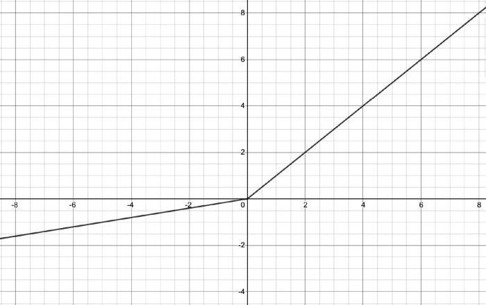
Stochastic Gradient Descent (SGD): As a result, the parameters of the model are updated in the following way:
A β represents the parameter of the model, and X and Y represent the input training data and labels, respectively. L stands for loss function and stands for learning rate. Each training example pair ( X, y ) is updated by SGD. In a variant of this method called mini-batch gradient descent, updates are performed every k examples, where k is the number of samples in the batch. For the whole mini-batch, gradients are calculated together. The batch gradient descent variant calculates the gradient across the whole dataset to update parameters.
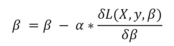
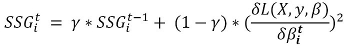
Adagrad: A single learning rate was used in the previous optimization schedule. When sparse data is present, some parameters may be more actively involved in feature extraction than others, making them need to be updated at different rates. Per-parameter updates are introduced by Adagrad, as shown below:

i is the ith parameter in the gradient descent iteration; t is the time step t of the iteration. In SSGit, the squared gradient for the ith parameter is summated from step 0 to step t. є indicates a small addition to the SSG to avoid division by zero. SSG allows the learning rate for frequently changing parameters to be reduced faster by dividing it by the square root.
Adadelta: Each time step in Adagrad adds squared terms to the denominator, increasing the learning rate. This leads to vanishingly small learning rates. To address this issue, Adadelta computes the sum of squared gradients only for previous time steps. The gradients of the past can be expressed as a decaying average:
For the previous sum of squared gradients, here is the decaying factor. Due to the decaying average, this formulation ensures that the sum of squared gradients does not accumulate to a large value. As soon as the SSG equation is defined, the Adagrad equation can be used to determine the update step for Adadelta.
If we look closely at the Adagrad equation, the root mean squared gradient is not dimensionless and thus the coefficient for learning rate should not be used. This problem can be resolved by defining another running average, this time for squared parameter updates. Here are the parameters that need to be updated:

To define the square sum of parameter updates, we can use the following equation, which is similar to the running decaying average of past gradients (the first equation under Adadelta):
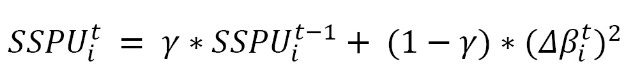
The sum of squared parameter updates is referred to as SSPU in this example. Adagrad’s dimensionality problem can be corrected with the final Adadelta equation:

There is no learning rate required in the final Adadelta equation. Learning rates can still be provided as multipliers, however. Due to this, the decaying factors are the only mandatory hyperparameters.
RMSprop: Due to the similarity between RMSprop and Adadelta, we have implicitly discussed its internal workings. In the Adagrad section, the update equation is obtained from the first equation in the Adadelta section, since RMSProp does not adjust for the dimensionality problem. In the case of RMSProp, we need to specify both a base learning rate and a decaying factor.
Adaptive Moment Estimation (Adam): A custom learning rate is calculated for each parameter in this optimization schedule. In the first equation in the Adadelta section, Adam also calculates decaying averages from the previous squared gradients, just like Adadelta and RMSprop. The decaying average of previous gradient values is also used:

Adaptive moment estimation consists of estimating the first and second moments of the gradient, which is equivalent to the SG and SSG. Usually, γ and γ’ are close to 1 and in that case, the initial values for both SG and SSG might be pushed towards zero. In order to counteract this, bias correction is applied to these two quantities:

Parameter updates are expressed as follows once they have been defined:

A decaying average of the gradient is used in place of the gradient on the extreme right-hand side of the equation. This optimization involves three hyperparameters — the base learning rate, gradient decay rates, and squared gradient decay rates. For training complex deep learning models, Adam has proven to be one of, if not the most, successful optimization schedule.
What should we use as an optimizer? Depending on the situation. Due to the per-parameter learning rate updates, adaptive optimizers (numbers 2 to 5) are beneficial with sparse data. Due to sparse data, parameter values might change at different rates, so a customized learning rate mechanism per parameter can greatly assist in achieving optimal results. It might also be possible to find a decent solution using SGD, but it will take a considerable amount of time to train. A monotonically increasing denominator in Adagrad leads to vanishing learning rates among the adaptive ones.
In terms of performance on various deep learning tasks, RMSProp, Adadelta, and Adam are quite similar. As with Adadelta, RMSprop uses the base learning rate instead of the decaying average of previous parameter updates, while Adadelta uses the decaying average of previous parameter updates. The Adam model is slightly different in that it accounts for bias correction as well as first-moment gradient calculation. Considering everything else equal, Adam might be the best optimizer.
Some of these optimization schedules will be used in this book’s exercises. By switching them with another one, you will observe the following changes:
Time and trajectory of model training (convergence)
The final performance of the model
The following chapters demonstrate how PyTorch can be used to solve different kinds of machine learning problems using these architectures, layers, activation functions, and optimization schedules. The example in this chapter includes convolutional, linear, max-pooling, and dropout layers in a convolutional neural network. All other layers are activated using ReLU and Log-Softmax as activation functions, respectively. A fixed learning rate of 0.5 is used with an Adadelta optimizer to train the model.
Exploring the PyTorch library
Based on the Torch library, PyTorch is a Python machine-learning library. In addition to being used for research, PyTorch is also used in the development of industrial applications. Facebook’s machine learning research labs are primarily responsible for its development. PyTorch competes with TensorFlow, which is developed by Google, the other well-known deep learning library. TensorFlow’s graph-based deferred execution was the initial difference between PyTorch and TensorFlow. The eager execution mode is also available in TensorFlow now.
Mathematical operations are computed immediately in eager execution, which is a form of imperative programming. All operations would be stored in a computation graph in a deferred execution mode, which would then be evaluated later. The advantages of eager execution include intuitive flow, easy debugging, and less scaffolding.
There is more to PyTorch than just deep learning. By utilizing GPU acceleration, it provides tensor computation capabilities with NumPy-like syntax and interface. How do tensors work? A tensor is a computational unit similar to a NumPy array, except that they can also be used on GPUs for accelerating computation.
The PyTorch deep learning framework provides accelerated computing and dynamic computational graphs. In addition, PyTorch is true Python-based, so users can take advantage of all Python’s features and the Python data science ecosystem.
A number of useful PyTorch modules can be found in this section that assist in loading data, building models, and specifying optimization schedules during model training. Furthermore, we will discuss how PyTorch implements tensors and their attributes.
PyTorch modules
Apart from offering the same computational functions as NumPy, PyTorch also provides a set of modules for quickly developing, training, and testing deep learning models. Modules that can be useful include the following.
torch.nn
Neural networks are built according to several fundamental aspects, such as the number of layers, the number of neurons in each layer, and whether they are learnable. By defining some of these high-level aspects, the PyTorch nn module simplifies the creation of neural network architectures instead of having to specify all the details manually. An example of an initialization of one-layer neural networks without using the nn module is as follows:

We can instead use nn.Linear(256, 4) to represent the same thing.
A submodule named torch.nn.functional exists within the torch.nn module. Unlike all the other submodules, this one contains all the functions in torch.nn. Loss functions, activating functions, and neural functions can all be used to create neural networks in a functional manner, where each layer is expressed as a function of the previous layer. This includes functions such as convolutional functions, linear functions, and pooling functions. Following are some examples of loss functions using torch.nn.functional:
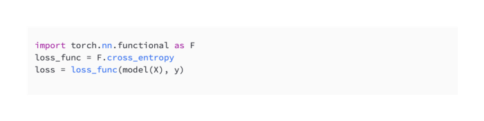
As shown in the example, X represents an input, Y represents an output, and the model represents a neural network model.
torch.optim
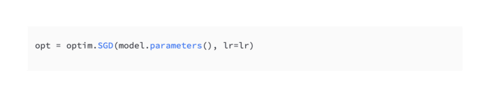
The process of optimizing neural networks involves back-propagating errors as we train them — the back-propagation of errors is the process of tuning their weights or parameters. As part of the deep learning training process, the optimize module includes all the tools and functionalities needed to run different optimization schedules. As shown in the following snippet, we can define an optimizer during a training session using torch.optim modules:
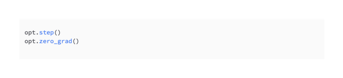
The optimization step can then be written automatically as shown here:
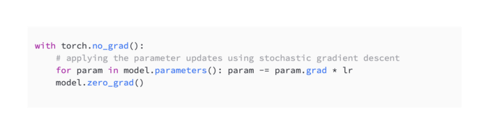
The following can be written instead:
Our next step will be to examine the utis.data module.
torch.utils.data
Torch provides its own dataset and DatasetLoader classes under its utis.data module. These classes are extremely useful thanks to their abstraction and flexibility. As a whole, these classes provide a simple and intuitive way to iterate over tensors and perform other such operations. Due to optimized tensor computations, we can achieve high performance while also ensuring failsafe data I/O. Consider the following example using torch.utils.data.DataLoader:

So instead of manually iterating through batches of data, we can do it automatically.

The following can be written instead:

The next step is to examine tensor modules.
Tensor modules
The concept of tensors is similar to that of NumPy arrays, as already mentioned. Tensors are n-dimensional arrays on which we can operate mathematical functions. Tensors can also be used to track gradients and computational graphs, which are useful for deep learning. We can run tensors on GPUs by casting them into a certain type.
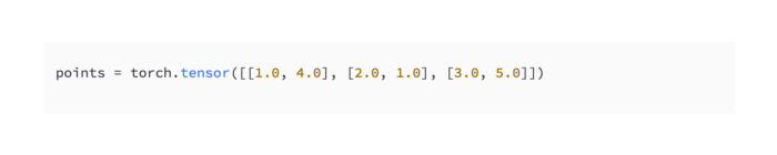
The following code shows how to instantiate a tensor in PyTorch:

The first entry can be retrieved by writing the following:

Here is another method for checking the tensor’s shape:

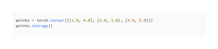
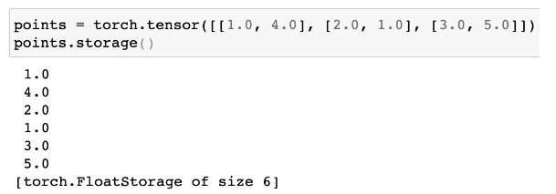
Several contiguous chunks of memory are used to store tensors in PyTorch as one-dimensional arrays. Storage instances are these arrays. This example shows how a PyTorch tensor can call its storage attribute to obtain the underlying storage instance for a tensor:
As a result, you should see:
The following information is used to implement the view of a tensor upon the storage instance:
Size
Storage
Offset
Stride
Our previous example can help us understand this:
This information can be interpreted in several ways:

As a result, you should see:
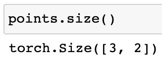
NumPy’s size attribute tells us how many elements are in each dimension, similar to NumPy’s shape attribute. These numbers are multiplied to equal the length of the underlying storage instance (6 here).
Now that we have seen what the storage attribute means, let’s take a look at offset:
As a result, you should see:
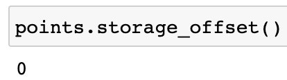
A tensor’s offset represents its index in the storage array as the first element of the tensor. 0 indicates that the array’s first element is the first element in the tensor, since it is 0 at the output.
Here’s what we need to know:

As a result, you should see:

The first element of the tensor is [2.0, 1.0], since points[1] is [2.0, 1.0] and the storage array is [1.0, 4.0, 2.0, 1.0, 3.0, 5.0]. There is an index 2 in the storage array for 2.0.
Lastly, let’s examine stride:

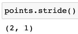
To access the next element of a tensor, stride indicates how many elements have to be skipped in each dimension. Using this example, we need to skip 2 elements (1.0 and 4.0) in order to reach the next element, 2.0, along the first dimension. To access the element after 1.0, we have to skip one element in the second dimension. A contiguous one-dimensional array can be used to create tensors using all these attributes.
A tensor is a collection of numeric data. The following types of data can be contained within tensors in PyTorch:
Torch.float32 or torch.float32 is a 32-bit floating-point type
Torch.float64 or torch.double is a 64-bit, double-precision floating point type
The torch.float16 and torch.half are 16-bit, half-precision floating-point functions
Signed 8-bit integers in torch.int8
Unsigned 8-bit integers in torch.uint8
Integers signed 16 bits, torch.int16 or torch.short
Signed 32-bit integers, torch.int32 or torch.int
Integers signed to 64 bits, torch.int64 or torch.long
The following is an example of how we specify the data type for a tensor:

A device specification is also necessary for PyTorch tensors, in addition to the data type. Devices can be instantiated in the following ways:

Alternatively, we can create a copy of the tensor in the desired device:

The two examples illustrate that we can either allocate tensors to CPUs (with device=’cpu’), which happens by default when nothing is specified, or to GPUs (with device=’cuda’).
The computation speed increases when tensors are placed on GPUs, and since PyTorch tensor APIs are largely the same for CPU and GPU tensors, moving them among devices to perform computations and move them back is quite convenient.
Using the device index, we can identify the device we want to place the tensor in if there are multiple devices of the same type, such as multiple GPUs.

With a thorough understanding of PyTorch and Tensor modules, we can now explore PyTorch’s neural network training module.
