Pandas One-liner Every Data Scientist Should Know

Pandas can be used to do a number of things in one line

Sep 23, 2022

∙ Paid

Today, it is easier than ever to train data-driven machine learning models. Take the case of a vanilla neural network that needs to be trained. With a slight modification to the model definition or its optimizer, you can adjust the architecture of the model for the number of hidden layers and their dimensions, tweak the hyperparameters, or change the loss function.

On one hand, this is advantageous because it eliminates having to spend time designing architectures from scratch. In contrast, researchers and practitioners of machine learning have often neglected the importance of data visualizations and analysis — training deep models without a clear understanding of their data.

This post will introduce you to a few powerful and essential one-liners specifically designed for tabular data using Pandas, which will help you gain a better understanding of your data and ultimately (hopefully) help you develop better machine learning models based on it.

The dataset

The dummy dataset for this post consists of a thousand employees which I created myself in Python. Our experiment dataset is shown in the image below.

I have implemented the following code block:

A Panda’s one-liner

To make sense of the data, let’s examine some popular Pandas functions.

#1 The n-largest value in a series

In this dataset, let’s find the top-n paid roles. The nlargest() method in Pandas can be used for this purpose. Using this method, you can retrieve the first n rows in descending order that have the largest values in column(s).

The nlargest() function returns the entire DataFrame, including columns that were not ordered. The DataFrame is not ordered using them, however. Below is a code snippet showing how to use the nlargest() method with a DataFrame.

n = 6
data.nlargest(n, "Employee Salary", keep = "all")

The final output must specify which particular row(s) should be included if duplicate values exist. Using the keep argument, this can be accomplished as follows:

If keep = “first”, the first occurrence will be prioritized.
Keep = “last”: prioritizes the most recent occurrence.
If keep = “all”, no duplicates are dropped, even if there are more than n items selected.

Many people make the mistake of thinking that nlargest() is exactly equivalent to sort_values():

n=6
data.sort_values(“Employee Salary”, ascending=False).head(n)

Nlargest(), however, relies on the keepargument. As shown above, nlargest() with keep=”all” will also return potential duplicates, while sort_values() will not.

A series of n-smallest values

Using Pandas’ nsmallest() method, you can find the rows corresponding to the lowest-n values similar to the nlargest() method. In ascending order, this method returns the first n rows with the smallest values in column(s). It takes the same arguments as nlargest(). In the code snippet below, we demonstrate how to use the nsmallest() method on our DataFrame.

n = 7
data.nsmallest(n, "Employee Salary", keep = "all")

CrossTabs

By default, Crosstab returns a frequency of each combination of columns/series based on a crosstabulation of two (or more). Crosstab() contains indexes for one column/list and column headers for another column/list based on its unique values. A function of aggregation is used to compute the values for each cell. Co-occurrences are indicated by default.

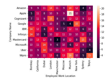
Suppose, for example, that we want to determine how many employees work from each location within every company. In order to accomplish this, follow these steps:

pd.crosstab(data["Company Name"], data["Employee Work Location"])

The following heatmap can be generated from a crosstab shown below, which makes numerical values easier to interpret (and more visually appealing):

result_crosstab = pd.crosstab(data["Company Name"], data["Employee Work Location"])
sns.heatmap(result_crosstab, annot=True)

The following example shows how to compute aggregation using a column other than those that make up the indexes and the column headers:

result_crosstab = pd.crosstab(index = data["Company Name"], 
                              columns=data["Employment Status"], 
                              values = data["Employee Salary"], 
                              aggfunc=np.mean)
                              
sns.heatmap(result_crosstab, annot = True, fmt = 'g')

Pivot Table

The pivot table is one of the most commonly used data analysis tools in Excel. Data can be cross-tabulated using pivot tables in Pandas, similar to crosstabs discussed earlier.

Despite their numerous similarities and conceptual similarities in Pandas, there are some implementational differences that make them distinct. The following code snippet demonstrates how to find the frequency of co-occurrence between “Company Name” and “Location” using pivot_table():

pd.pivot_table(data, 
               index=["Company Name"], 
               columns=["Employee Work Location"], 
               aggfunc='size', 
               fill_value=0)

Heatmaps can be created similarly to Crosstab to make them visually appealing and more interpretable. The following heatmap can be generated by following the code snippet:

result_pivot = pd.pivot_table(data, 
                              index=["Company Name"], 
                              columns=["Employee Work Location"], 
                              aggfunc='size', 
                              fill_value=0)
               
sns.heatmap(result_pivot, annot = True, fmt = 'g')

Onepagecode