The purpose of this blog post is to introduce the design of a machine learning algorithm that can forecast stock market crashes solely from past price information. My approach and findings are summarized after providing a quick background on the problem. Code and data can be found on the GitHub repository.
Dear Subscribers,
First of all thank you everyone who became a subscriber. Now I have got 48 free subscribers and 2 paid subscribers. We did it in just one month. So I have decided to make some changes to the articles. Now I will provide readers with a link to the aws s3 bucket where you can download the source code of each article, complete code with all data source and citation and pdf support documents, everything. But only subscribers will be able to download it. So please make sure you are subscribed, it helps. From the next article, you can find a link at the bottom of the article where you can download it.
Typically, stock market crashes occur when a market drops more than 10% in value within a short period of time. Black Monday in 1987 and the housing bubble in 2008 are popular examples of major stock market crashes. In general, a crash occurs when a price bubble bursts and there is a massive sell-off of assets when most market participants attempt to sell at the same time.
Inefficient markets can be inferred from the presence of price bubbles. Prices in inefficient markets are not always indicative of fundamental asset values, but are inflated or deflated depending on traders' expectations. Traders' subsequent actions reinforce these expectations by increasing (or decreasing) prices. This results in inflated (or deflated) prices. George Soros described this phenomena as reflexivity, which is the underlying assumption of technical analysis forecasting.
Currently, there is not much debate over whether financial markets have bubbles. In spite of this, predicting price bubbles and understanding inefficiencies is a challenging task. Think about being able to identify when the market is about to crash and predict when the bubble will burst. In addition to making profits when prices are increasing, you would be able to avoid losses when the time comes to sell.
Mathematicians and physicists have explored the mathematics behind price structures in an attempt to solve this problem. Professor Didier Sornette has predicted multiple financial crashes successfully [1]. To describe how price bubbles form and burst, Sornette uses log-periodic power laws (LPPLs). Accordingly, the LPPL fits price changes ahead of a crash to a faster-than-exponentially increasing function with a log-periodic component (presumably reflecting price volatility as it increases in magnitude and frequency).
It is from here that the idea for this project comes. Should it not be possible for a machine learning algorithm to learn these patterns and predict crashes if the recurring price structures found by researchers exist? This algorithm would not have to know the mathematical laws that govern the underlying physical processes, but be trained on data from crashes that have already been identified, and would identify and learn these patterns by itself.
Data and Crashes
Collecting financial data and identifying crashes was the first step. Stock quotes from low-correlated major markets were used. Testing and cross-validating models require low cross-correlation. Below is the cross-correlation between daily stock market returns from 11 major markets.
For the purpose of excluding data from any two sets with a cross-correlation greater than 0.5 in my collection, I selected only data from the S&P 500 (USA), the Nikkei (Japan), the HSI (Hong Kong), the SSE (Shanghai), the BSESN (India), SMI (Switzerland) and the BVSP (Brazil).
I first calculated price drawdowns for each data set in order to identify crashes. Drawdowns occur when the price continuously declines from the last price maximum to the next price minimum over a period of consecutive days. The following chart illustrates three such drawdowns that occurred in the S&P 500 over the period from end of July to mid August 2018.
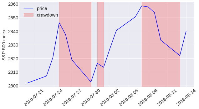
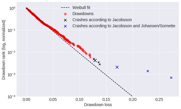
Two methodologies were considered to identify crashes. Emilie Jacobsson identified the first crash as a drawdown in the 99.5% quantile in each market. The drawdown thresholds I found using this methodology range from around 10% for less volatile markets such as the S&P 500 to over 20% for volatile markets such as Brazil. When plotting the logarithm of the rank of drawdowns in a data set versus magnitude, Johansen and Sornette identify crashes as outliers, that is drawdowns that differ from the fitted Weibull distribution.
I tested my algorithms using both crash identification methods and determined that the first methodology (Jacobsson) offers two advantages. As a first point, Sornette doesn't specify the amount of deviation from the Weibul distribution that constitutes a crash, so a human judgment is required. As a result of his methodology, fewer crashes are identified, resulting in a greatly imbalanced data set. As a result, it is more difficult to gather enough data to train a machine learning algorithm.
The collection of these seven datasets provided me with a total of 59,738 rows of daily stock prices, allowing me to identify 76 crashes.
Problem statement and feature selection
To determine whether a crash will occur within a specific period of time (e.g. each trading day), I formulated a classification problem.
The information to make a prediction on a certain day can be gathered by analyzing the daily price changes of all days preceding that day. A feature that can be used to preempt a crash on day t is the daily price change from the day prior to t. However, since too many features can lead to slower and less accurate models ("curse of dimensionality"), it is advisable to extract just the most relevant features at any given point in time. Thus, I calculated mean price changes over the past year (252 trading days) for each day using eight different time windows. From 126 days (for t-126 to t-252), I used increasing window sizes to obtain a higher resolution of recent price changes. I added eight features to represent the mean price volatility over the same time frames since price volatility is not captured when averaging price changes over multiple days. The mean price changes and volatilities for each data set were normalized.
Analyzing the regression coefficients of a logistic regression allowed me to evaluate the feature selection. Logistic regression coefficients correspond to the logarithm of how the odds of a crash (the ratio of the probability of a crash versus not crashing) change as a function of the associated feature when all other variables are held constant. I converted the log odds to odds for the plot below. An increase in a corresponding feature increases the crash probability greater than 1.
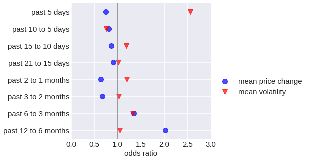
According to the coefficient analysis, the recent volatility is the strongest predictor of an impending crash. Even though prices have recently increased, there appears to be no crash imminent. At first glance, this seems surprising since a bubble is typically characterized by an exponential increase in price. However, many of the crashes found did not occur immediately after a price peak, rather, prices decreased gradually before the crash. Price movements over longer time periods contain valuable information for crash forecasting, as a general price increase over the long term makes a crash more likely. Additionally, a high price increase in the past 6 to 12 months is also associated with a predicted crash.
Training, validation, and test set
For testing, I selected the S&P 500 data set, and for training and validation, I selected the remaining six data sets. Choosing the S&P 500 for testing was due to the size of the data set (daily price information from 1950) and the number of crashes (20). I performed cross-validation training six times. Using six data sets for each model, five for training and one for validation, each model was run six times.
Scoring
I used the F-beta score to evaluate each model's performance. Precision and recall are weighted harmonic means for the F-beta score. They are determined by the beta parameter. When the beta is greater than one, recall is prioritized, and when the beta is smaller, precision is prioritized.
Beta 2 puts more emphasis on recall, which means a predicted crash that does not happen gets a stronger punishment than an undetected crash. In the risk averse view, it makes sense to assume that not predicting a crash that occurs will have more severe consequences (loss of money) than expecting a crash that doesn't happen (loss of profits).
Regression models, Support vector machines and Decision trees
My first step was to create linear and logistic regression models. The goal of a regression model is to minimize the difference between the predicted value and the actual value over the whole training set. Logistic regression estimates probabilities rather than continuous variables. Thus, it is better suited to classification problems than linear regression. The results of both models were almost identical, but in some cases, logistic regression outperformed linear regression. Despite this being a surprise, it is important to note that even if logistic regression provides a better fit to estimate crash probability, a linear regression with a non-optimal fit would not be a disadvantage in practice if the chosen threshold effectively separated binary predictions. F-beta score was maximized by optimizing this threshold on the training set.
//////////
My next step was to test Support Vector Machines (SVMs). The kernel function of SVMs is used to project the input features into a multidimensional space and determine a hyperplane to place positive and negative samples. There are a number of parameters to think about: the penalty parameter C (measures how much misclassification can be avoided), the kernel function (polynomial or radial basis function), the kernel coefficient gamma (determines the size of the kernel function), and the class weight (determines how positive and negative predictions are balanced). SVM models with the highest scores achieved similar results to regression models. The faster training time of regression models makes them more attractive. With any of the other models tested, decision trees were not able to match their performance.
Recurrent Neural Networks
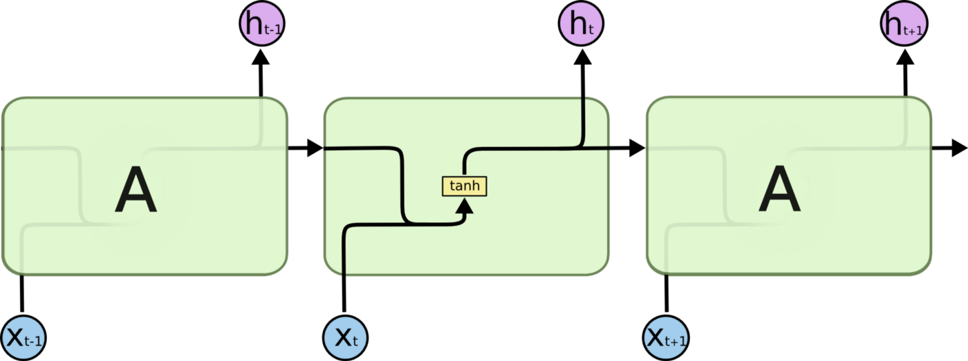
Implementing recurrent neural networks (RNNs) was the next step. Contrary to traditional machine learning algorithms and traditional artificial neural networks, recurrent neural networks can take into consideration the order in which data is received and thus allow information to persist. It seems that this is one of the most crucial characteristics of an algorithm that deals with time series data, such as daily stock returns. Through loops, cells are connected so that at time-step t, the input is not only the feature xt but also the output from the previous time-step ht-1. This concept is illustrated in Figure 1.
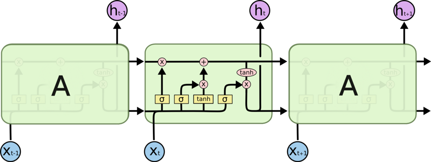
However, the major problem with RNNs is that they cannot learn long-term dependencies. Ht may not be able to learn anything from xt-n if there are too many steps between them. To assist with this, Long Short Term Memory (LSTM) networks have been developed. LSTMs do not only pass the output of the previous cell ht-1 to the next cell, but also the "cell state" ct-1 as well. Each time the cell state is updated, it relies on the input (xt and ht-1) to update the output (ht). The interactions between inputs xt, ht-1, and ct-1 and the outputs ht and ct are handled by four neural network layers in each LSTM cell. Please see colah's blog for a detailed description of LSTM cell architecture.
Simple regression models are not capable of detecting relationships or patterns that RNNs with LSTMs can. As such, if an RNN LSTM could learn the price structures which precede crashes, wouldn't it be able to outperform the previously tested models?
With the Python library Keras, I implemented two different RNNs with LSTMs and went through a rigorous hyper-parameter tuning process. First, I had to determine how long each layer's input would be. For each time step t, daily price changes are taken from a sequence of days that have preceded t. It is important to choose this number carefully since longer input sequences require more memory and slow down computation. While an LSTM implementation in Keras should be able to detect long-term dependencies, the cell states are only passed from one sequence to the next if the parameter stateful is set to true. Such a design is inconvenient in practice. The state of the network was manually reset whenever the training data switches data sets in order to avoid that it recognizes long-term dependencies spanning over multiple data sets and epochs during training. Since this algorithm did not provide significant results, I changed stateful to false and added additional sequences of average price changes and mean volatility to the network from time windows before 10 days up to 252 days ago (similar to features selected for the previous tested models). I also experimented with different loss functions, the number of layers, the number of neurons per layer, and dropped out vs no dropped out. A RNN LSTM with the best performance has two LSTM layers of 50 neurons each, the Adam optimizer, a cross-entropy loss function, and a sigmoid activation function for the last layer.
Evaluation
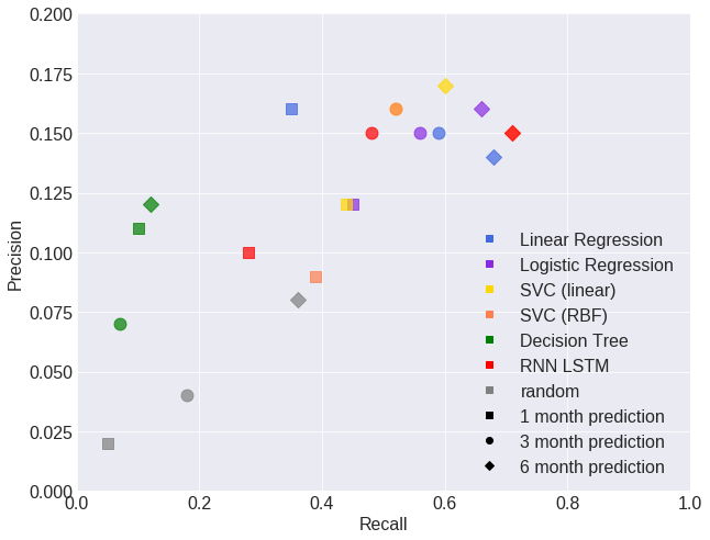
Even though hyper parameter tuning, increasing sequence lengths, and adding long term features lead to faster training (optimal results on the validation set after around 10 epochs), none of the RNN LSTM models outperformed the previous models.
The plot above shows the performance of the different models in terms of precision and recall. The color and shape of the case indicate a different model (crash in 1, 3 or 6 months). The graph below shows the F-beta scores of all models for crash predictions after 1, 3 and 6 months. Random refers to a model without predictive power that predicts as many crashes as the tested models.


