

Predicting Stock Prices With Deep Neural Network
This project walks you through the end-to-end data science lifecycle of developing a predictive model for stock price movements with Alpha Vantage APIs and a powerful ML Algo called LSTM.

By completing this project, you will learn the key concepts of machine learning / deep learning and build a fully functional predictive model for the stock market, all in a single Python file.
#@title Load Python libraries

! pip install alpha_vantage -q

# pip install numpy
import numpy as np

# pip install torch
import torch
import torch.nn as nn
import torch.nn.functional as F
import torch.optim as optim
from torch.utils.data import Dataset
from torch.utils.data import DataLoader

# pip install matplotlib
import matplotlib.pyplot as plt
from matplotlib.pyplot import figure

# pip install alpha_vantage
from alpha_vantage.timeseries import TimeSeries

print("All libraries loaded")
This code uses specific tools to help with processing and modeling data in Python. These tools are used for analyzing and displaying information numpy, matplotlib, teaching computers torch, and getting financial information alpha_vantage. The first part of the code silently installs the alpha_vantage tool using -q. The rest of the code brings these tools into the current working space. The code also includes other useful parts from the torch tool, like the torch.nn part for designing neural networks, torch.optim for improving them, and torch.utils.data for creating data sets. The code also uses TimeSeries from the alpha_vantage tool, but only for collecting financial time-series data. Finally, the code prints a message to show that everything has loaded smoothly.
config = {
    "alpha_vantage": {
        "key": "YOUR_API_KEY", # Claim your free API key here: https://www.alphavantage.co/support/#api-key
        "symbol": "IBM",
        "outputsize": "full",
        "key_adjusted_close": "5. adjusted close",
    },
    "data": {
        "window_size": 20,
        "train_split_size": 0.80,
    },
    "plots": {
        "show_plots": True,
        "xticks_interval": 90,
        "color_actual": "#001f3f",
        "color_train": "#3D9970",
        "color_val": "#0074D9",
        "color_pred_train": "#3D9970",
        "color_pred_val": "#0074D9",
        "color_pred_test": "#FF4136",
    },
    "model": {
        "input_size": 1, # since we are only using 1 feature, close price
        "num_lstm_layers": 2,
        "lstm_size": 32,
        "dropout": 0.2,
    },
    "training": {
        "device": "cpu", # "cuda" or "cpu"
        "batch_size": 64,
        "num_epoch": 100,
        "learning_rate": 0.01,
        "scheduler_step_size": 40,
    }
}
This code creates a dictionary named config that holds important details about the alpha vantage API, data, plots, model, and training. The alpha vantage API part includes the API key, stock symbol, size of output, and adjusted closing value. The data section includes the size of the window and the split for training. The plots section has instructions for showing graphs, displaying tick intervals, and color-coding. The model part includes specifications for the neural network, like input size, number of LSTM layers, size of LSTM, and rate of dropout. Lastly, the training section holds information for training the model, such as device CPU or GPU, batch size, number of epochs, learning rate, and scheduler step size.
Data Preparation: Acquiring Financial Market Data From Alpha Vantage
def download_data(config, plot=False):
    # get the data from alpha vantage

    ts = TimeSeries(key=config["alpha_vantage"]["key"])
    data, meta_data = ts.get_daily_adjusted(config["alpha_vantage"]["symbol"], outputsize=config["alpha_vantage"]["outputsize"])

    data_date = [date for date in data.keys()]
    data_date.reverse()

    data_close_price = [float(data[date][config["alpha_vantage"]["key_adjusted_close"]]) for date in data.keys()]
    data_close_price.reverse()
    data_close_price = np.array(data_close_price)

    num_data_points = len(data_date)
    display_date_range = "from " + data_date[0] + " to " + data_date[num_data_points-1]
    print("Number data points:", num_data_points, display_date_range)

    if plot:
        fig = figure(figsize=(25, 5), dpi=80)
        fig.patch.set_facecolor((1.0, 1.0, 1.0))
        plt.plot(data_date, data_close_price, color=config["plots"]["color_actual"])
        xticks = [data_date[i] if ((i%config["plots"]["xticks_interval"]==0 and (num_data_points-i) > config["plots"]["xticks_interval"]) or i==num_data_points-1) else None for i in range(num_data_points)] # make x ticks nice
        x = np.arange(0,len(xticks))
        plt.xticks(x, xticks, rotation='vertical')
        plt.title("Daily close price for " + config["alpha_vantage"]["symbol"] + ", " + display_date_range)
        plt.grid(b=None, which='major', axis='y', linestyle='--')
        plt.show()

    return data_date, data_close_price, num_data_points, display_date_range

data_date, data_close_price, num_data_points, display_date_range = download_data(config, plot=config["plots"]["show_plots"])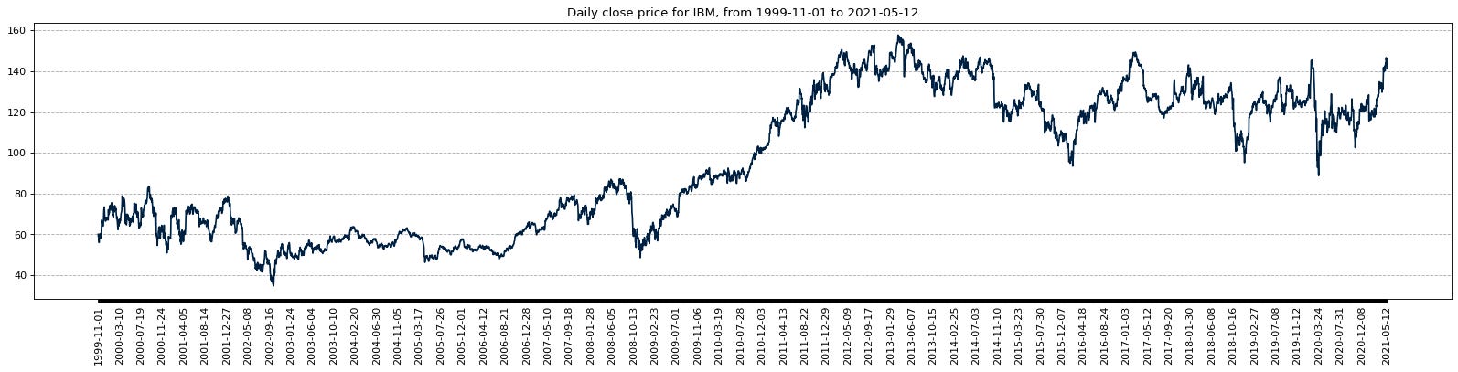
This code is a tool that retrieves information from the Alpha Vantage website by using a chosen setup. It needs input for the setup and has an option to show the information in a graph. Inside, it takes the information from the Alpha Vantage site and keeps it organized in variables. Then, it arranges the information in order starting from the most recent date and stores the date and price values in separate groups. After that, it calculates the number of information points and displays a message showing the date range. If the graph option is turned on, the code will use matplotlib to display the information. It also adjusts the size and background of the graph and formats the dates on the x-axis to be evenly spaced and rotated. In the end, the graph is shown and it returns the date, price, number of data points, and display message.
Data preparation: Normalising Raw Financial Data
class Normalizer():
    def __init__(self):
        self.mu = None
        self.sd = None

    def fit_transform(self, x):
        self.mu = np.mean(x, axis=(0), keepdims=True)
        self.sd = np.std(x, axis=(0), keepdims=True)
        normalized_x = (x - self.mu)/self.sd
        return normalized_x

    def inverse_transform(self, x):
        return (x*self.sd) + self.mu

# normalize
scaler = Normalizer()
normalized_data_close_price = scaler.fit_transform(data_close_price)
This code is used to make things easier for us, by creating a Normalizer helper. This helper has two ways to do things: fit_transform and inverse_transform. The __init__ way inside of the helper gets things ready for us by starting off with nothing for the mu and sd things. These are used to remember the average and the difference from the average for the numbers. The fit_transform way gets a set of numbers called x and figures out the average and the difference from the average using the numpy thing. It then makes the numbers normal by taking away the average from each one and then dividing by the difference. We keep this new set of normal numbers in a thing called normalized_x. The inverse_transform way takes the normal numbers and changes them back by doing the opposite things, like multiplying by the difference and then adding back the average. This makes the numbers go back to how they were before. In the end, we use this helper by creating one of it and using the fit_transform way to make the numbers in the data_close_price set normal.
