Predicting the Future with Deep Learning: A Practical Guide to Timeseries Forecasting

From naive baselines and sliding-window datasets to LSTMs, GRUs, recurrent dropout, and bidirectional encoders — everything you need to build causally valid, production-ready forecast models in Keras.

Download the entire book using the button at the end of this article

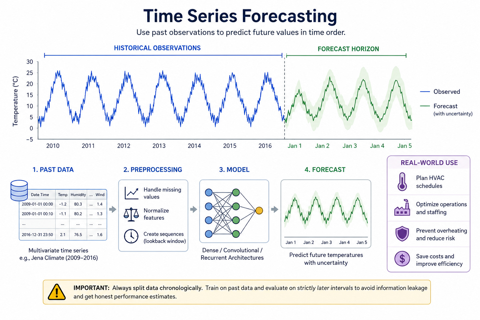
A timeseries is any sequence of measurements taken at ordered points in time. Each observation can be a single scalar (for example, temperature recorded once per hour) or a vector of features (temperature, humidity, wind speed, and so on). What distinguishes timeseries data from ordinary tabular data is that the order of records matters: nearby observations are typically correlated, and patterns unfold over time. That temporal structure is precisely what forecasting models aim to capture.

Typical tasks applied to timeseries data fall into a few broad categories. Forecasting predicts future values of one or more series given past observations. Anomaly detection flags points or intervals that deviate from normal behavior. Classification assigns a label to an entire sequence (for example, determining whether a heartbeat trace indicates arrhythmia). Event detection locates and timestamps occurrences of specific events inside a long stream. Each task exploits the temporal ordering in different ways; forecasting explicitly models how past dynamics influence the future.

This chapter concentrates on forecasting. Forecasting matters because many real-world systems need forward-looking decisions: inventory planning relies on demand forecasts, power grids schedule generation ahead of load predictions, preventive maintenance depends on estimating when a temperature or vibration trend will cross a safety threshold. Accurate short- and medium-range forecasts enable operational efficiency, cost savings, and risk reduction.

Consider a concrete industrial monitoring scenario: a factory records temperature from many sensors every ten minutes. The operations team wants to predict the next day’s temperature pattern for a cooling zone to plan HVAC schedules and staffing. A successful forecast lets the team pre-cool or delay workloads, avoiding spikes that would trip alarms or reduce equipment lifetime. The relevant model must learn temporal dependencies in the temperature series — for instance, daily cycles, trends after machinery starts, and slow changes caused by ambient conditions — and produce predictions sufficiently far ahead to be actionable.

A critical methodological caveat applies to all tasks on ordered data: treating temporally ordered records as independent and identically distributed (i.i.d.) typically produces misleadingly optimistic validation results. Randomly shuffling or globally reordering rows breaks causality and leaks future information into the training set, corrupting model evaluation. Always split data chronologically for validation and test: training on past data and evaluating on strictly later intervals preserves the temporal forecasting problem and yields honest estimates of real-world performance.

With those foundations in place — what a timeseries is, how forecasting differs from other tasks, and why forecasting is operationally important — the remainder of the chapter builds an end-to-end forecasting workflow. You will see how to prepare temporal data without leaking information, establish simple baselines, and compare dense, convolutional, and recurrent architectures while maintaining proper time-aware validation.

Temperature forecasting problem setup and dataset

Start by downloading the Jena Climate CSV and extracting it into the working directory. The dataset used throughout the chapter is the Jena climate time series (2009–2016).

!wget https://s3.amazonaws.com/keras-datasets/jena_climate_2009_2016.csv.zip
!unzip -o jena_climate_2009_2016.csv.zip

This creates the file jenaclimate2009_2016.csv. Listing the working directory after running the commands should show that CSV file.

A quick sanity check reads the header and counts timesteps. The first column must be the timestamp ("Date Time"); the remaining columns are numeric features.

csv_path = 'jena_climate_2009_2016.csv'
with open(csv_path, 'r', encoding='utf-8') as fh:
    lines = fh.read().strip().split('\n')
header_cells = lines[0].split(',')
record_count = len(lines) - 1
print('header:', header_cells)
print('rows (excluding header):', record_count)
assert header_cells[0] == 'Date Time'
assert record_count > 1

The printed header shows the field names (15 tokens including the timestamp) and the record count verifies you have rows to work with. The assertions enforce that the file looks like the expected Jena CSV.

Next parse the CSV into a NumPy feature matrix and extract the temperature column as the target vector. The CSV rows contain the timestamp followed by 14 numeric feature columns; the temperature feature is at column index 1 (after the timestamp). We build a featuresmat with shape (numtimesteps, 14) and a tempvec with shape (numtimesteps,).

import numpy as np
csv_path = 'jena_climate_2009_2016.csv'
with open(csv_path, 'r', encoding='utf-8') as fh:
    rows = fh.read().strip().split('\n')
header = rows[0].split(',')
content = rows[1:]
num_steps = len(content)
num_features = len(header) - 1  # exclude Date Time
features_mat = np.zeros((num_steps, num_features), dtype='float32')
temp_vec = np.zeros((num_steps,), dtype='float32')
for i, r in enumerate(content):
    cells = r.split(',')
    vals = np.asarray(cells[1:], dtype='float32')
    features_mat[i, :] = vals
    temp_vec[i] = vals[1]  # temperature at column index 1
print(features_mat.shape, temp_vec.shape)
assert features_mat.shape[1] == 14
assert features_mat.shape[0] == temp_vec.shape[0]

The shapes printed should reflect one row per observation and fourteen numeric features per row (for example, (420551, 14) and (420551,) when the dataset is present). The explicit extraction temp_vec[i] = vals[1] fixes the temperature feature index as 1; downstream code and evaluation will rely on this index for un-normalizing predictions.

Split the data chronologically. For timeseries forecasting you must preserve causality: do not randomly shuffle rows or compute normalization statistics on the entire dataset. A simple, reproducible temporal split is first 50% for training, next 25% for validation, and final 25% for testing. Compute the split sizes from the total row count so slicing is deterministic and clearly preserves time order.

# Assume features_mat and temp_vec exist as built earlier
total = features_mat.shape[0]
train_count = total // 2
val_count = total // 4
# temporal split: first 50% train, next 25% val, last 25% test

Using the dataset sizes above, the typical sample counts are: numtrainsamples: 210225; numvalsamples: 105112; numtestsamples: 105114

(These counts demonstrate a 50/25/25 chronological split. Always derive these from the actual total so your slices remain consistent when using slightly different versions of the data.)

Normalize features using statistics computed strictly on the training slice, and keep the per-feature mean and standard deviation vectors for later un-normalization. Computing mean/std on the entire dataset leaks information from the future into the model and produces over-optimistic validation/test metrics.

import numpy as np
# Assume features_mat and temp_vec exist as built earlier
total = features_mat.shape[0]
train_count = total // 2
val_count = total // 4
# temporal split: first 50% train, next 25% val, last 25% test
mean_vec = features_mat[:train_count].mean(axis=0)
std_vec = features_mat[:train_count].std(axis=0)
scaled = (features_mat - mean_vec) / std_vec
# sanity on training slice only
train_scaled = scaled[:train_count]
res_mean = np.abs(train_scaled.mean(axis=0)).max()
res_std = np.abs(train_scaled.std(axis=0) - 1.0).max()
print('max |mean| on train slice:', float(res_mean))
print('max |std-1| on train slice:', float(res_std))
assert res_mean < 5e-3
assert res_std < 5e-2

This normalization computes meanvec and stdvec only from the training portion and applies that transform to all data. Keep meanvec and stdvec (particularly the temperature feature's entries meanvec[1] and stdvec[1]) to un-normalize temperature predictions later: predictedtemperature = preds * stdvec[1] + mean_vec[1]. If you forget to un-normalize using the temperature feature's training mean/std, your reported MAE and other metrics will be incorrect.

A couple of common pitfalls to avoid: computing normalization statistics on the whole dataset or reordering rows (for example, global shuffling) both break temporal causality and leak future information into model training and validation. Always compute normalization parameters on the training slice only and perform chronological splits for training, validation, and testing.

Create timeseries datasets

A timeseries forecast problem is most naturally expressed as a sliding-window mapping: a fixed-length recent history (the window) is presented as input and the model is trained to predict a value some steps into the future. The Keras utility keras.utils.timeseriesdatasetfrom_array creates exactly these overlapping windows for training and evaluation, and it also aligns targets relative to each input window so supervision is correct.

Start with a tiny integer sequence to see how a single-step alignment works. The snippet below builds windows of length 3 and sets the target to be the element 3 steps ahead of the start of each window. This makes the mapping concrete: [0, 1, 2] → 3 for the first sample.

import numpy as np
from tensorflow import keras
seq = np.arange(10)
windows = seq[:-3]
targets = seq[3:]
ds = keras.utils.timeseries_dataset_from_array(
    data=windows,
    targets=targets,
    sequence_length=3,
    batch_size=2
)
for batch_x, batch_y in ds.take(1):
    print('X[0]:', batch_x[0].numpy())
    print('y[0]:', batch_y[0].numpy())
    assert list(batch_x[0].numpy()) == [0, 1, 2]
    assert int(batch_y[0].numpy()) == 3

Running this prints the first input window and its aligned target; the assertions verify that the dataset has produced the mapping you expect. This demonstrates two core ideas: sequence_length controls the length of the input history, and the dataset utility aligns targets relative to windows rather than simply pairing arbitrary slices.

When building a real forecasting dataset from multivariate, chronologically ordered measurements, three parameters matter in particular: samplingrate, sequencelength, and the delay between the end of the input window and the target. samplingrate selects how frequently to sample observations from the original high-frequency stream when assembling a window. sequencelength is the number of sampled timesteps per window. delay is how far ahead in the original data the target lies, expressed in raw timesteps. For a 24-hour-ahead forecast on data sampled every 10 minutes, a sampling_rate of 6 gives roughly one sample per hour (6 × 10 minutes = 1 hour). Using hourly samples reduces redundancy in the window compared with keeping every 10-minute point while still retaining the diurnal structure important for weather forecasting.

Be explicit about the arithmetic. For a history of five days sampled hourly, sequence_length = 120 (5 days × 24 hours). To forecast 24 hours ahead you want the target 24 sampled steps after the window's last sampled step; because delay is expressed in raw timesteps you compute:

delay = samplingrate * (sequencelength + 24 - 1)

The +24-1 accounts for the off-by-one relationship between window endpoints and target indexing in this setup.

Below is a practical instantiation that creates temporally consistent train / validation / test datasets for the Jena-style dataset (assume scaled, tempvec, meanvec, stdvec, and counts are already prepared in the same environment). The required settings appear explicitly: samplingrate = 6, sequencelength = 120, delay computed as shown, and batchsize = 256.

import numpy as np
from tensorflow import keras
# scaled, temp_vec, mean_vec, std_vec, and counts assumed prepared as above
sampling_rate = 6
sequence_length = 120
delay = sampling_rate * (sequence_length + 24 - 1)
batch_size = 256
n = scaled.shape[0]
train_count = n // 2
val_count = n // 4
start_train = 0
end_train = train_count
start_val = end_train
end_val = end_train + val_count
start_test = end_val
end_test = n
inputs = scaled[:-delay]
future = temp_vec[delay:]
train_ds = keras.utils.timeseries_dataset_from_array(
    data=inputs,
    targets=future,
    sampling_rate=sampling_rate,
    sequence_length=sequence_length,
    start_index=start_train,
    end_index=end_train,
    shuffle=True,
    batch_size=batch_size
)
val_ds = keras.utils.timeseries_dataset_from_array(
    data=inputs,
    targets=future,
    sampling_rate=sampling_rate,
    sequence_length=sequence_length,
    start_index=start_val,
    end_index=end_val,
    shuffle=False,
    batch_size=batch_size
)
test_ds = keras.utils.timeseries_dataset_from_array(
    data=inputs,
    targets=future,
    sampling_rate=sampling_rate,
    sequence_length=sequence_length,
    start_index=start_test,
    end_index=end_test,
    shuffle=False,
    batch_size=batch_size
)
for xb, yb in train_ds.take(1):
    print('samples shape:', xb.shape)
    print('targets shape:', yb.shape)
    assert xb.shape[1:] == (sequence_length, scaled.shape[1])
    assert yb.shape[0] == xb.shape[0]

On the first batch you should see a printed sample shape that matches the batch size and window dimensions—typically something like:

samples shape: (256, 120, 14); targets shape: (256,)

The assertions confirm that each sample has sequence_length time steps and the same number of features as the scaled input array, and that there is exactly one target per input sample.

Two practical cautions are worth emphasizing here. First, the two lines inputs = scaled[:-delay] and future = tempvec[delay:] are tightly coupled: if they are mismatched you will train on misaligned supervision. A common mistake is to slice inputs and targets inconsistently, which silently corrupts training. Second, design your batchsize with care. Very small batch sizes can produce noisy validation curves and make it harder to interpret improvement or overfitting; using a moderate batch_size such as 256 gives more stable evaluation while remaining efficient on typical GPUs and TPUs.

Finally, keep chronological splits when you set startindex and endindex: never mix temporal order when creating validation or test sets. The timeseriesdatasetfromarray parameters startindex, end_index, and shuffle control that chronology: use shuffle=True only for training windows (and even then within the training slice) and keep shuffle=False for validation and test datasets so that evaluation always reflects forward-in-time performance.

Commonsense baseline (naive forecast = last observed temperature)

A simple, informative baseline for a forecasting task is the persistence (or "last observed value") forecast: predict that the temperature at the target horizon will equal the last observed temperature in the input window. This requires no learning and gives a concrete MAE to compare every trained model against.

The persistence forecast must be computed in the original temperature units, so you must un-normalize the last observed temperature from each input window before comparing it to the ground-truth target. The temperature column is column index 1; given meanvec and stdvec computed on the training split, un-normalize with preds * stdvec[1] + meanvec[1]. Forgetting to un-normalize here produces an MAE that is meaningless.

The following function iterates over a tf.data Dataset of (inputs, targets) batches, extracts the last observed (normalized) temperature at xb[:, -1, 1], un-normalizes it, and accumulates absolute errors to compute MAE across the dataset. It assumes valds and testds plus meanvec and stdvec are already available from the data-preparation steps described earlier.

import numpy as np
# Requires val_ds, test_ds, mean_vec, std_vec from previous steps
def mae_for(ds):
    total_err = 0.0
    count = 0
    for xb, yb in ds:
        # last observed temperature at column index 1 (normalized); un-normalize prediction
        last_temp_norm = xb[:, -1, 1].numpy()
        preds = last_temp_norm * std_vec[1] + mean_vec[1]
        total_err += np.abs(preds - yb.numpy()).sum()
        count += preds.shape[0]
    return total_err / count

val_mae = mae_for(val_ds)
test_mae = mae_for(test_ds)
print('Baseline MAE: Validation', round(float(val_mae), 2), 'Test', round(float(test_mae), 2))
assert abs(val_mae - 2.44) < 0.25
assert abs(test_mae - 2.62) < 0.25

When you run this, expect the baseline MAE to be roughly 2.44 on validation and 2.62 on test. The provided assertions allow a modest tolerance while anchoring the numbers to the reported references. Use this persistence MAE as the minimum bar: any model you train should aim to beat this no-learning forecast.

Dense model baseline

A compact fully connected regressor provides a simple learning baseline for a timeseries forecasting task. The model below flattens the sequence dimension so the network sees the last 120 timesteps as a long feature vector, then reduces it through a small hidden layer to a single scalar prediction. This setup intentionally discards the temporal ordering inside the window, so it tests how much signal is available if the model can only rely on aggregated, order-agnostic patterns.

The following code constructs the model using the Functional API, compiles it with mean squared error loss while tracking mean absolute error as a readable performance metric, and adds a ModelCheckpoint callback that saves the best validation-MAE weights to the file jena_dense.keras.

from tensorflow import keras
from tensorflow.keras import layers
inputs = keras.Input(shape=(120, 14))
x = layers.Flatten()(inputs)
x = layers.Dense(16, activation='relu')(x)
outputs = layers.Dense(1)(x)
dense_model = keras.Model(inputs, outputs)
dense_model.compile(optimizer='adam', loss='mse', metrics=['mae'])
ckpt = keras.callbacks.ModelCheckpoint('jena_dense.keras', save_best_only=True, monitor='val_mae', mode='min')
# Fit using the datasets from earlier
# history = dense_model.fit(train_ds, validation_data=val_ds, epochs=10, callbacks=[ckpt])
# test_metrics = dense_model.evaluate(test_ds)
# print('Test MAE (dense):', test_metrics[1])
dense_model.summary()

Line-by-line: keras.Input(shape=(120, 14)) declares the expected input shape: a window of 120 timesteps with 14 features per timestep. layers.Flatten() converts that (120, 14) tensor into a single vector of length 120*14 so subsequent Dense layers operate on a fixed-length feature vector. The hidden Dense(16, activation='relu') is a small bottleneck that limits model capacity and encourages the model to extract compact patterns from the flattened vector. The final Dense(1) produces the scalar target prediction.

Choosing loss='mse' optimizes squared error, which is appropriate for regression and tends to produce smooth predictions; metrics=['mae'] records mean absolute error during training and validation, which is easy to interpret in the original units of your target once you un-normalize predictions. ModelCheckpoint('jenadense.keras', savebestonly=True, monitor='valmae', mode='min') ensures the saved weights correspond to the lowest validation MAE observed during training, simplifying later evaluation and preventing you from accidentally evaluating an overfitted final checkpoint.

Because Flatten removes time-order information inside the window, this model cannot learn sequence-dependent behaviors such as phase shifts or trends across timesteps. If the forecasting signal primarily depends on recent ordering or on temporal dynamics, you should expect this dense baseline to perform no better (and often worse) than a simple naive baseline that uses the last observed temperature; the dense model's MAE often ends up close to the naive baseline. That closeness is a useful diagnostic: it tells you the benefit of modeling temporal order is likely necessary for improved forecasts.

A practical warning: with small architectures like this, training for many epochs without regularization commonly produces overfitting—training loss can continue to fall while validation MAE stalls or increases. Using ModelCheckpoint to preserve the best validation weights mitigates some risk, but you should still monitor the validation curve and consider stronger regularization, early stopping, or architectures that respect temporal structure (convolutions or recurrent layers) if validation performance does not improve.

After fitting, inspect densemodel.summary() to verify the Flatten, Dense(16), and Dense(1) layers appear as expected and confirm the ModelCheckpoint callback points to 'jenadense.keras'. When you evaluate the saved best model on your test split, un-normalize any predictions back to the original temperature units before reporting MAE; forgetting to un-normalize will give an incorrect error measure.

1D ConvNet baseline

Treat the timeseries as a one-dimensional signal and apply temporal convolutions, then pool to reduce temporal resolution and finish with a regression head. Convolutional filters scan short windows of history and can learn local temporal patterns; pooling progressively reduces the temporal dimension so later layers summarize broader-context features.

The following model stacks three Conv1D layers with progressively smaller kernel sizes (24, 12, 6). MaxPooling1D halves the temporal length between the first two blocks, and a GlobalAveragePooling1D aggregates the last feature map into a single vector for a Dense(1) regression output. This exact sequence — Conv1D, MaxPooling1D, Conv1D, MaxPooling1D, Conv1D, GlobalAveragePooling1D, Dense(1) — is important for the behavior discussed below.

from tensorflow import keras
from tensorflow.keras import layers

inp = keras.Input(shape=(120, 14))
y = layers.Conv1D(8, 24, activation='relu')(inp)
y = layers.MaxPooling1D(2)(y)
y = layers.Conv1D(8, 12, activation='relu')(y)
y = layers.MaxPooling1D(2)(y)
y = layers.Conv1D(8, 6, activation='relu')(y)
y = layers.GlobalAveragePooling1D()(y)
out = layers.Dense(1)(y)

conv_model = keras.Model(inp, out)
conv_model.compile(optimizer='adam', loss='mse', metrics=['mae'])
conv_model.summary()
# When trained, expect validation MAE around 2.9, underperforming baselines.

Read the code as a sequence of transformations on a (timesteps, features) input. The first Conv1D with kernel size 24 inspects 24 time steps at a time and produces 8 feature maps. MaxPooling1D(2) reduces temporal length by a factor of two, which increases the effective receptive field of subsequent convolutions while shrinking resolution. The later Conv1D layers use smaller kernels (12 then 6) to refine patterns at coarser scales. GlobalAveragePooling1D collapses the time axis entirely by averaging each feature map across time; the Dense(1) head converts that summary into the scalar forecast.

Temporal convolution and pooling are attractive because they let the model process many timesteps in parallel (better throughput than recurrent layers) and they encode a form of local translation invariance: a feature detected at one temporal position is treated similarly if it appears elsewhere. But that very translation invariance can be a liability for forecasting tasks. Forecasting commonly relies on precise temporal order and the absolute position of recent events: pooling and global averaging can wash out the fine-grained ordering information the model needs to make accurate short-horizon predictions.

Because GlobalAveragePooling1D collapses the time axis, the model must encode all necessary ordering cues into feature activations before that averaging step; if those cues are subtle or localized near the end of the input window, averaging may blur them. In practice, on the temperature forecasting task used throughout this chapter, this Conv1D+pooling design typically yields a validation MAE around 2.9 — worse than much simpler baselines such as small recurrent or dense-window models.

When you train this architecture, inspect the model.summary() output to confirm the kernel sizes and pooling structure: the Conv1D layers should show kernel_size values 24, 12, and 6, and you should see MaxPooling1D layers between the first and second Conv1D blocks. This structure is what causes the aggressive temporal downsampling and the resulting trade-off between broad context and preserved ordering.

A practical warning for model design: do not assume that translation invariance and pooling are always beneficial for forecasting. Pooling can remove critical temporal ordering information, harming predictive performance even when the model looks more powerful on paper. If you need to preserve the relative ordering of recent events, prefer architectures that maintain higher temporal resolution (smaller pooling, causal convolutions without aggressive pooling, or recurrent layers that preserve timestep outputs) rather than applying global pooling too early.

Introduce RNNs and LSTM on the task

Train a compact LSTM regressor that improves on the naive and dense baselines by letting the model learn temporal dependencies in the input sequences.

An LSTM layer processes a sequence of vectors and emits a summary vector (unless you ask it to return the full sequence). That summary carries information about past timesteps through the layer’s internal cell state (the carry). The cell update follows the standard LSTM update equation: c{t+1} = it k_t + c_t ft where it is the input gate, kt is the candidate content, ft is the forget gate, and ct is the previous cell (carry). The carry ct is distinct from the layer’s output (the hidden state); the two are related but not identical, and conflating them can lead to confusion when stacking or inspecting LSTMs.

Below is a compact example: an input for 120 timesteps with 14 features, a single LSTM layer with 16 units, and a Dense(1) regression head. The model is compiled with optimizer='adam', loss='mse', and metrics=['mae']. A ModelCheckpoint saves the best model to 'jena_lstm.keras' by monitoring validation MAE.

from tensorflow import keras
from tensorflow.keras import layers
inn = keras.Input(shape=(120, 14))
h = layers.LSTM(16)(inn)
reg = layers.Dense(1)(h)
lstm_model = keras.Model(inn, reg)
lstm_model.compile(optimizer='adam', loss='mse', metrics=['mae'])
ckpt = keras.callbacks.ModelCheckpoint('jena_lstm.keras', save_best_only=True, monitor='val_mae', mode='min')
# history = lstm_model.fit(train_ds, validation_data=val_ds, epochs=10, callbacks=[ckpt])
# test_metrics = lstm_model.evaluate(test_ds)
# print('Test MAE (LSTM):', test_metrics[1])
lstm_model.summary()

Key lines and what they do:

• keras.Input(shape=(120, 14)) declares the expected input shape: 120 timesteps, 14 features per timestep (temperature is the second column in the dataset preprocessing used earlier).

• layers.LSTM(16) creates an LSTM layer with 16 units; by default it returns the last output for the sequence, which we pass to the Dense regressor.

• model.compile(optimizer='adam', loss='mse', metrics=['mae']) configures training with mean-squared error loss and mean absolute error as a human-readable metric.

• ModelCheckpoint('jenalstm.keras', savebestonly=True, monitor='valmae', mode='min') saves the best validation-MAE model to disk so you can restore the best weights after training.

If you run the training step against the prepared training, validation, and test datasets, this compact model typically surpasses the naive baseline and the dense baseline: validation MAE is usually around 2.39 and test MAE around 2.55 for the same preprocessing and data splits used earlier. Those numbers are empirical outcomes of training this specific architecture on the prepared temperature forecasting setup and will vary with different preprocessing, sequence lengths, or dataset slices.

A couple of practical cautions. LSTMs and other recurrent networks can overfit quickly if you give them excessive capacity or train many epochs without regularization; monitor validation MAE and use callbacks such as EarlyStopping or a ModelCheckpoint as shown. Also remember the difference between cell carry and output when designing stacked RNNs: if you stack recurrent layers, you must use return_sequences=True on lower layers so the next layer receives a full sequence rather than a single vector.

RNN mechanics

A recurrent layer runs the same small neural network at every timestep, passing a compact state from one timestep to the next. At each step the layer consumes the input at that timestep and the previous state, computes a new state (and typically an output), then hands that new state forward to the next timestep. This per‑timestep recurrence is the core mechanics behind SimpleRNN, LSTM, and GRU cells.

The following NumPy snippet implements the SimpleRNN recurrence explicitly so you can see the loop and the state update in plain Python. It computes an output for each timestep as tanh(xt · W + state{t} · U + b) and replaces the running state with that output.

import numpy as np
# SimpleRNN forward pass (mechanics demo)
T, in_f, out_f = 5, 3, 4
x_seq = np.arange(T * in_f, dtype='float32').reshape(T, in_f) / 10.0
W = np.ones((in_f, out_f), dtype='float32') * 0.1
U = np.ones((out_f, out_f), dtype='float32') * 0.05
b = np.zeros((out_f,), dtype='float32')
state_t = np.zeros((out_f,), dtype='float32')
outputs = []
for t in range(T):
    output_t = np.tanh(x_seq[t].dot(W) + state_t.dot(U) + b)
    state_t = output_t
    outputs.append(output_t)
outputs = np.stack(outputs, axis=0)
print('outputs shape:', outputs.shape)
assert outputs.shape == (T, out_f)
assert np.allclose(state_t, outputs[-1])

What this code shows, step by step:

• The loop iterates over timesteps t = 0..T-1. At each step you compute a new outputt from the current input xseq[t] and the previous state statet. The tanh activation is applied to the linear combination xt·W + state_t·U + b.

• The running state is replaced by outputt. For this SimpleRNN formulation the layer's hidden state and its per‑timestep output are the same vector; the assertion at the end confirms statet equals the last timestep's output.

• The outputs list collects an output for every timestep and stacking along axis 0 produces an array of shape (T, out_f). The print and assertions check that shape and the final-state property.

Per‑timestep recurrence is the mechanism for temporal memory: information from earlier inputs influences later outputs only through the state that is passed forward. In SimpleRNN the state update is exactly output_t = tanh(...), but LSTM and GRU implement more sophisticated gating to control what information is kept, forgotten, or exposed.

State propagation and output shapes are important when you build multi‑layer recurrent networks. A single recurrent layer applied to an input sequence typically returns either:

• a single vector (the final state / final output) when return_sequences=False, or

• a sequence of vectors (one per timestep) when return_sequences=True.

In Keras API terms, SimpleRNN, LSTM, and GRU all accept the returnsequences flag. By default returnsequences=False, meaning the layer outputs only the last timestep's vector. Setting return_sequences=True makes the layer return the full sequence of outputs with shape (timesteps, units) for a single sample (or (batch, timesteps, units) in batched mode).

This distinction matters when you stack recurrent layers. Consider two recurrent layers, RNN1 followed by RNN2. RNN2 expects a sequence as input (one vector per timestep). If RNN1 is configured with returnsequences=False, it will produce just a single vector and you get a shape mismatch when feeding that into RNN2. To stack RNN layers you must set returnsequences=True on every recurrent layer except the final one so that each intermediate layer produces a sequence that the next layer can consume. In short: for stacking, return_sequences=True on all but the last recurrent layer.

Common mistake: forgetting return_sequences=True when stacking leads to immediate shape errors or accidental removal of temporal context. The former happens because the next recurrent layer receives a 2‑D tensor (batch, features) instead of a 3‑D tensor (batch, timesteps, features); the latter is a logical error if you intended deeper temporal processing but cut the sequence to a single vector prematurely.

A separate but related concept is statefulness across batches. A Keras recurrent layer can operate in stateless mode (the default) where the hidden state is reset between batches, or in stateful mode where the layer preserves its last state and uses it as the initial state for the next batch. Stateful mode can be useful when you feed a very long sequence in smaller batches while preserving temporal continuity, but it requires careful management (e.g., manually resetting states between independent sequences) and has constraints: batch size must be fixed and you must maintain chronological batch ordering. Also note that recurrent features such as recurrent_dropout may influence performance and available fast implementations (for example, some GPU-optimized kernels are disabled when certain dropouts are enabled).

Remember the API names: SimpleRNN, LSTM, and GRU implement the recurrent cell types; returnsequences controls whether a layer returns the full output sequence or only the final output. When stacking, set returnsequences=True on intermediate layers to preserve the per‑timestep outputs that the deeper layers need.

From SimpleRNN to LSTM cell anatomy

An LSTM cell maintains two distinct channels of information as it processes a sequence: a persistent carry (often written c_t) that is designed to store long-term, slowly changing information, and a hidden output channel that exposes a filtered version of the cell's state at each timestep. The cell controls updates to the carry with three learned gating signals computed from the current input and the previous hidden state. These gates are commonly named i (input gate), f (forget gate), and k (candidate, sometimes written g). Each gate is a vector of values between 0 and 1 that modulates how information flows into, out of, and within the carry.

Think of it as "how much new content to write" into the carry at time t, ft as "how much of the existing carry to keep," and k_t as "what new candidate content could be written." The combination of these three gates gives the exact update rule for the carry. Written compactly, the carry update is:

ct+1 = it k_t + c_t f_t.

Read this equation term by term. The product it * kt is the gated new content: candidate content kt scaled by the input gate it, so only a fraction determined by it will be added. The product ct * ft is the retained content: the previous carry ct scaled by forget gate ft, so the cell can choose to decay or preserve parts of the carry. Together they sum to the next carry ct+1, meaning the cell can both forget some past information and add new information at the same timestep.

This persistent carry is the structural reason LSTMs resist the vanishing gradient problem that plagues plain recurrent networks. Because the carry update is an explicit, nearly-additive recurrence — each new carry is the previous carry scaled plus an additive term — gradients flowing back through many timesteps can propagate via multiplicative factors f_t close to 1 without being repeatedly squashed by nonlinearities. In other words, the carry provides a direct highway for error signals to travel many steps backward in time, preserving information about long-range dependencies that standard recurrent units would gradually lose.

The separation between the carry and the visible hidden output is important. The carry ct is an internal memory; the hidden output (often denoted ht) is a transformed, gated version of that memory exposed to the next layer or to a prediction head. Because they serve different roles, confusing ct with the hidden output leads to misunderstandings about how an LSTM stores and exposes information. Practically, the cell can keep a slowly evolving trend in ct while letting transient, short-term fluctuations affect h_t and thereby the network's immediate outputs.

A concrete intuition helps. Consider temperature forecasting where the underlying climate trend (a slowly changing baseline across months or years) matters alongside daily fluctuations. The long-term trend is the precise kind of information kept in the carry: by setting ft values near 1 for components representing the trend and keeping it small for those components, the LSTM can preserve that baseline across many timesteps. Short-term variations — a cold front, a heat spike — can be represented transiently in the hidden output ht by allowing those components to be strongly influenced by kt and it for a few steps, then decay back to the stored trend as ft restores the carry. In this way, the network can answer both "what is the slow-moving baseline?" and "what short-term deviations are occurring now?" without destroying the long-term memory.

Remember that the gates themselves are learned functions of input and previous hidden state; they allow the model to dynamically decide when to memorize, when to forget, and when to expose memory to the outside. This flexibility is what makes LSTMs effective on tasks requiring memory over many timesteps: sequences where relevant signals can appear far apart in time, yet must be integrated to produce accurate forecasts.

Finally, keep a practical warning in mind: carry ct and the cell's hidden output ht are related but distinct. When analyzing or debugging LSTM behavior, inspect both channels conceptually. If you want to reason about long-term storage and gradient flow, focus on the carry and its update rule (ct+1 = it k_t + c_t ft). If you want to understand what the network is emitting at each step for immediate predictions, examine the hidden outputs and the output gate that controls how the carry is filtered into ht. Confusing these two will lead to incorrect interpretations of how an LSTM preserves or discards information.

Advanced RNN usage: recurrent dropout, stacking, bidirectionality

A simple way to regularize an LSTM is to combine recurrent dropout (a dropout mask applied to the recurrent state) with standard Dropout on the layer outputs. Recurrent dropout masks the recurrent connections so that the hidden-to-hidden updates are stochastically thinned at each timestep, while a Dropout layer after the RNN thins the information passed to downstream layers or the final readout. Note that using recurrent_dropout disables the cuDNN fast path for RNNs, which can make training noticeably slower even though the regularization often helps generalization.

The following model shows this pattern: an LSTM with recurrent_dropout, a Dropout head, and a Dense scalar output. The checkpoint saves the best validation MAE.

from tensorflow import keras
from tensorflow.keras import layers
x_in = keras.Input(shape=(120, 14))
z = layers.LSTM(32, recurrent_dropout=0.25)(x_in)
z = layers.Dropout(0.5)(z)
z_out = layers.Dense(1)(z)
rd_model = keras.Model(x_in, z_out)
rd_model.compile(optimizer='adam', loss='mse', metrics=['mae'])
ckpt = keras.callbacks.ModelCheckpoint('jena_lstm_dropout.keras', save_best_only=True, monitor='val_mae', mode='min')
# history = rd_model.fit(train_ds, validation_data=val_ds, epochs=50, callbacks=[ckpt])
# test_metrics = rd_model.evaluate(test_ds)
# print('Test MAE (LSTM+recurrent_dropout):', test_metrics[1])
rd_model.summary()
print('Note: recurrent_dropout disables cuDNN fast path; training is slower.')

What to look for in this snippet: recurrentdropout=0.25 supplies the recurrent mask applied to the LSTM's carry/hidden transitions; layers.Dropout(0.5) drops half of the LSTM outputs before the Dense readout. The ModelCheckpoint callback name must match exactly if you want to resume or inspect saved weights. When trained on the Jena temperature task with the same data preprocessing as the earlier experiments, this model typically requires more epochs to converge because the regularization slows overfitting; observed validation MAE in a complete run is roughly 2.27 and test MAE roughly 2.45. Remember the practical trade-off: enabling recurrentdropout removes access to the fast CuDNN kernel, so expect slower step times.

If you need more capacity while still trying to control overfitting, stacking recurrent layers is a natural next step. Stacking means the lower recurrent layer must return its full sequence of hidden states so the upper recurrent layer can consume temporal information at each timestep. Forgetting to set return_sequences=True on the lower layer is a common shape bug: the upper layer expects a sequence input but receives a single vector per sample instead.

Here is a compact stacked-GRU example that increases depth while applying recurrent dropout to both GRU layers and a final Dropout before the Dense output. Notice that return_sequences=True is set on the first GRU so the second GRU receives a sequence.

from tensorflow import keras
from tensorflow.keras import layers
inp = keras.Input(shape=(120, 14))
s1 = layers.GRU(32, recurrent_dropout=0.5, return_sequences=True)(inp)
s2 = layers.GRU(32, recurrent_dropout=0.5)(s1)
s2 = layers.Dropout(0.5)(s2)
out = layers.Dense(1)(s2)
gru_model = keras.Model(inp, out)
gru_model.compile(optimizer='adam', loss='mse', metrics=['mae'])
# history = gru_model.fit(train_ds, validation_data=val_ds, epochs=50)
# test_metrics = gru_model.evaluate(test_ds)
# print('Test MAE (stacked GRU):', test_metrics[1])
gru_model.summary()

Key implementation points for stacked GRUs: the first GRU uses return_sequences=True, which produces shape (batch, timesteps, units) suitable for the second GRU. The second GRU by default returns its last output (a vector per sample), which is then regularized and mapped to the scalar prediction. In practice, adding depth can improve modeling capacity and sometimes reduce test MAE (in an experiment on this dataset a stacked GRU achieved test MAE around 2.39), but deeper models can also overfit quickly if the signal-to-noise ratio is low and regularization is insufficient.

Finally, consider bidirectional RNNs. Wrapping an LSTM (or GRU) in a Bidirectional layer runs one recurrent pass left-to-right and another right-to-left, then concatenates (or otherwise combines) the two final states. This is powerful when the prediction for a token depends on both past and future context relative to that token: classical sequence-labeling tasks such as named-entity recognition or part-of-speech tagging often benefit substantially from bidirectional encoders because the relevant evidence may be on either side of the target position.

The next snippet builds a Bidirectional LSTM that outputs a single prediction after combining forward and backward passes:

from tensorflow import keras
from tensorflow.keras import layers
xin = keras.Input(shape=(120, 14))
h = layers.Bidirectional(layers.LSTM(16))(xin)
y = layers.Dense(1)(h)
bidir = keras.Model(xin, y)
bidir.compile(optimizer='adam', loss='mse', metrics=['mae'])
# history = bidir.fit(train_ds, validation_data=val_ds, epochs=10)
# test_metrics = bidir.evaluate(test_ds)
# print('Test MAE (BiLSTM):', test_metrics[1])
bidir.summary()

Why bidirectional models can harm causal forecasting: bidirectional RNNs access future timesteps relative to the prediction point during the backward pass, which breaks the causal assumption required for forecasting. For next-step or horizon forecasting where only past data should inform the prediction, incorporating future information during training yields overly optimistic patterns that cannot be used during live inference. In experiments on the temperature forecasting task above, a Bidirectional LSTM often performs worse than a comparable unidirectional model because it encourages learning of features that exploit symmetric context rather than causal temporal dynamics.

When bidirectionality is appropriate, however, it is invaluable. Named-entity recognition is a concrete example: whether a token is an entity often depends on words both before and after it (for example, titles that follow names, or disambiguating context words). Bidirectional(LSTM) in those sequence-labeling architectures aggregates context from both sides and improves per-token classification accuracy.

A final set of practical caveats and runtime trade-offs to remember when experimenting with recurrent models:

• recurrentdropout disables cuDNN fast kernels for RNNs. Training will still be correct, but per-step throughput will be slower. Use recurrentdropout when you need recurrent regularization, but expect longer wall-clock times.

• unroll=True requests unrolled recurrent loops in the graph; unrolling requires a fixed sequence length at model build time and increases graph size. Do not set unroll=True if you plan to feed variable-length sequences.

• return_sequences=True is required on intermediate RNN layers in a stack. Omitting it on a lower layer leads to a shape mismatch because the subsequent RNN expects a time-distributed input.

• Recurrent-dropout masks are applied to the recurrent connections (hidden-to-hidden). Dropout layers applied after RNN outputs are independent and drop input-to-output activations; use both when you want to regularize different parts of the computation.

These patterns—recurrent dropout, output Dropout, stacked recurrent layers with return_sequences on lower layers, and cautious use of bidirectional wrappers—give you a practical toolkit for moving from lightweight sequence models to deeper encoders while keeping an eye on causality and runtime behavior.

Further improvements and caveats

Forecasting models can often be improved by careful tuning and better inputs, but there are realistic limits: some signals simply aren’t predictable from available observations. When you evaluate possible improvements, treat each change as an experiment with a clear, causally valid evaluation protocol so you don’t mistake leakage for genuine progress.

A few levers to explore systematically are the length of history the model sees, the model’s capacity (hidden sizes and depth), the set of input features, and the strength and type of regularization. History length controls how much past context the network can use. Short windows bias the model toward local, short-term patterns; long windows enable learning daily or weekly periodicities but increase the risk of overfitting and raise computational cost. Try a logarithmic sweep of window sizes (for example, 1 hour, 6 hours, 24 hours, 3 days, 7 days) rather than only tiny incremental changes — different phenomena often appear at very different scales.

Hidden-size and depth changes trade capacity for overfitting risk. Increasing the number of units in an LSTM/GRU or adding stacked recurrent layers can let the model represent more complex temporal dependencies, but it also provides more degrees of freedom to memorize noise. When stacking recurrent layers remember the API constraint: lower recurrent layers must return sequences (returnsequences=True) so upper layers receive a time series rather than a single vector; otherwise you’ll hit shape errors. Empirically, moderate increases in hidden size often help up to a point, after which validation error worsens. If validation error starts to climb, add dropout, recurrentdropout (with the caveat that recurrent_dropout disables cuDNN fast paths and slows training), L2 weight decay, or reduce layer width before blindly adding depth.

Feature engineering frequently buys more than model tinkering. Raw temporal signals rarely contain everything the model needs. Add deterministic calendar features (hour-of-day, day-of-week, holidays), lagged values at key lags (for example, values at 24h and 168h for daily and weekly cycles), rolling statistics (means, variances over recent windows), and external covariates such as temperature or occupancy. Carefully derive features so they are causal: every feature must be computable using only data available at prediction time. Computing normalization statistics or engineered features across the entire dataset leaks future information and produces over-optimistic validation; compute means and standard deviations on the training slice and reuse them for validation and test. Maintain chronological splits in all future experiments.

Evaluation for time series needs different tooling than iid problems. Standard k-fold cross-validation that shuffles rows destroys causality. Use forward-chaining (rolling or expanding window) validation: train on an initial period, validate on the immediately following period, then roll the split forward. This reproduces the operational setting in which you make predictions on genuinely unseen future data. Report both pointwise errors (MAE, RMSE) and errors aggregated over meaningful time horizons (for example, daily MAE when you forecast hourly) so you understand operational impact. Also inspect residuals for structure: persistent biases at certain hours or days indicate missing features or mis-specified seasonality.

Hyperparameter search should respect time structure. Random and Bayesian search often outperform grid search on expensive models because they explore more variety for the same budget. When you use automated search, wrap the training loop so each trial computes validation error on a forward-chaining split. Keep the search budget realistic: training deep recurrent models for many epochs is costly, and small batch sizes can introduce noisy validation curves that make comparisons unreliable. Use early stopping based on the time-aware validation set, and log checkpoints so you can resume or inspect intermediate models.

Baselines matter. A simple persistence model (predicting that the future equals the last observed value) or a linear autoregressive baseline often captures much of the predictable structure in physical systems like temperature or electrical demand. Compare every candidate neural model against these strong, simple baselines; without them you risk celebrating a complex model that barely beats naïve predictions. Assuming additional depth always helps is a common mistake: complexity without a better signal usually increases variance rather than accuracy.

There are realistic performance bounds intrinsic to the domain and the features you possess. Physical processes with slow dynamics and strong periodicity — temperature, energy demand, some load forecasts — are often predictable at short horizons because they’re driven by consistent patterns and external covariates. Financial markets or events driven by high-noise human behavior may be close to unpredictable at the timescale and feature set you have; complex models will mostly fit noise. When you see modest improvements in validation error from very large models, ask whether the improvement is meaningful for your application or just statistical noise.

Windowed forecasting is a transferable workflow. Consider an energy demand forecasting example: given hourly smart meter data, predict total demand 24 hours ahead. Use a window of recent hourly observations and augment it with calendar features (hour, weekday) and lagged signals at 24 and 168 hours to capture daily and weekly periodicities. Train models with the same forward-chaining validation, starting with simple baselines and then trying a small dense network, a convolutional model that captures short-term motifs, and a recurrent model that captures longer dependencies. For many such problems the same sequence of steps — build causal features, keep chronological splits, establish strong baselines, then increase model complexity while monitoring validation behavior — transfers cleanly.

Finally, logging and interpretability are practical guards. Keep a reproducible record of dataset slices, normalization parameters, hyperparameters, and training checkpoints. Visualize predictions aligned with inputs so you can see when models follow seasonality versus when they latch onto spurious fluctuations. That discipline, combined with chronologically valid evaluation and careful feature design, is the most reliable path from experimental improvements to models that behave well in production.

Use the button below to download the book as pdf