

Quant Trading: Kyle’s Price Impact & Order Flow Alpha Generation (Python Guide)
Estimating microstructure price impact, signed order flow, and Amihud illiquidity for stock return forecasting.

Download the Source Code Using the URL At the End of This Article
The paper estimates Kyle's price-impact coefficient from CRSP daily equity data and tests whether order-flow-based measures forecast contemporaneous and subsequent monthly stock returns. It constructs signed order flow, total volume, volume volatility, a within-month price-impact regression estimator, and an Amihud-style illiquidity estimator. The theoretical interpretation is that adverse selection and temporary price impact, rather than only risk compensation, can generate an illiquidity premium.
Implementation Assumptions
Required CRSP, H.15, WRDS, factor, and delisting datasets are supplied locally as files; no network access or credentials are used.
PERMNO and calendar-month keys are the canonical identifiers throughout the empirical pipeline.
The default sample period is 2020–2025 when the available data support it.
The default expanding-window interpretation is used because the procedural description explicitly specifies expansion, despite occasional use of the word rolling.
The default empirical lambda regression is uncentered because Equation 12 displays no intercept; this choice is exposed in configuration because the paper is ambiguous.
Zero daily price changes receive sign zero.
Firm-month winsorization scope is configurable and never silently assumed.
Newey–West lag length, covariance treatment, portfolio weighting, and missing-data rules are explicit configuration fields because they are unspecified in the supplied paper extraction.
OCR-damaged equations eq3, eq6, eq8, and eq16 are not reconstructed beyond the supplied meanings and prose.
Reported paper coefficients and summary statistics are stored as comparison targets, not as independently reproduced results.
No code execution, numerical verification, or semantic validation is claimed under the supplied run policy.
Scope, evidence boundaries, and pipeline architecture
What would it take to turn the paper’s liquidity and return-predictability tests into a reproducible Python workflow? The practical answer is not one model call. It is a chain of contracts: local daily records are cleaned, daily activity is summarized by firm and calendar month, estimators are aligned with subsequent returns, and each analysis produces labeled outputs with provenance.
The paper studies whether observable trading activity contains information about contemporaneous and future stock returns. Its structural motivation comes from Kyle-style price impact: informed and noise trading combine into signed aggregate order flow, and a market maker adjusts prices in response. The empirical data do not reveal those latent theoretical orders separately. Instead, the reproduction uses signed daily volume as an observable proxy, alongside unsigned volume, volume volatility, and two firm-month illiquidity or price-impact estimators.
This distinction is central. The theoretical aggregate flow is a model quantity; the empirical signedflow column is constructed from CRSP observations. Likewise, lambda is not one universally defined field. Its meaning depends on whether it was produced by the within-month price-impact regression or by the Amihud-style average.
The evidence boundary
The supplied paper describes a principal sample covering 2020–2025 and reports coverage and regression results, including firm and firm-month counts. Those values are paper-reported comparison targets, not independently reproduced results in this workflow. A full numerical reproduction requires local CRSP data and, for particular analyses, H.15 risk-free rates, WRDS book-to-market and factor data, and possibly delisting-return and point-in-time membership files.
The implementation therefore follows three categories:
Paper facts: the stated sample period, exchange filter, minimum 15 nonzero-volume-day firm-month rule, daily-to-monthly feature definitions, and the planned regression and forecast families.
Implementation decisions: the exact adjustment-field convention, unchanged-price sign handling, winsorization scope, covariance treatment, forecast pooling, Newey–West lag, and portfolio weighting.
Unavailable evidence: missing source data, incomplete adjustment instructions, and OCR-damaged or underspecified parts of the paper.
The code keeps the second category in configuration rather than silently choosing hidden behavior. It also avoids filling missing data with paper-reported values. The package is local-only: it reads files supplied by the user and does not access a network or credentials.
The pipeline as an accounting ledger
The canonical identifiers are PERMNO, the CRSP firm identifier, and month, a normalized calendar-month key. The intended data flow is:
daily CRSP rows
    -> filtered and adjusted daily rows
    -> daily dollar volume, signed flow, and Amihud ratios
    -> one row per (PERMNO, month)
    -> lambda estimates, returns, and controls
    -> contemporaneous and next-month model inputs
    -> regressions, forecasts, portfolios, and reports
Every transition should answer four questions:
What source columns were used?
What is the resulting row shape and key?
Which time period does each value describe?
Which convention controls missing or ambiguous values?
The generated ReproductionConfig records many of these choices. Its defaults are explicitly described as conventions rather than uniquely paper-determined facts:
@dataclass(frozen=True)
class ReproductionConfig:
    """Validated settings for local data preparation and empirical analyses.

    Defaults reflect implementation decisions made where the supplied paper
    extraction is ambiguous: a 2020--2025 sample, exchanges 1/2/3, a
    15-nonzero-volume-day filter, an uncentered lambda estimator, zero sign for
    unchanged prices, monthly winsorization, equal-weighted deciles, and no
    assumed covariance correction.  These defaults are not claimed to be the
    paper's uniquely specified conventions.
    """

    sample_start: DateLike = "2020-01-01"
    sample_end: DateLike = "2025-12-31"
validate_config checks ranges and supported options, but it does not establish that a local file exists or that its contents match the paper’s sample. That separation matters: configuration validation is not empirical verification.
What each orchestration layer does
build_empirical_panel(config) is the main preprocessing boundary. It loads the configured CRSP daily and monthly files, applies exchange and date filters, constructs adjusted prices and daily features, aggregates firm-month variables, estimates both lambda columns, attaches available controls, applies configured winsorization, and creates same-firm next-month targets. Its output should contain at most one row for each PERMNO-month pair.
run_empirical_reproduction(panel, config) receives that normalized panel rather than loading data itself. It isolates model-specific inputs and delegates to the empirical modules:
pooled contemporaneous and one-month-ahead return regressions;
lambda-return regressions for both estimators and intercept variants;
firm-level expanding-window forecasts and pooled forecast evaluation;
monthly Fama–MacBeth regressions and signal-sorted decile portfolios.
The reporting layer, build_reproduction_report(panel, results, config), assembles coverage, descriptive, regression, forecast, and portfolio tables. Its design keeps computed outputs separate from paper targets. A target annotation can describe a comparison value, but it must not overwrite a locally computed coefficient or observation count.
The two command-line entry points reflect this separation. scripts/build_panel.py constructs auditable daily and firm-month artifacts. scripts/run_reproduction.py builds or loads a panel, runs the model pipeline, and writes report tables. Neither command is evidence that execution occurred here; they are local interfaces for a future run with suitable data.
A small worked example: one firm through the ledger
Consider a synthetic firm with PERMNO equal to 10001 and three daily observations in January. The rows might contain the following conceptual fields
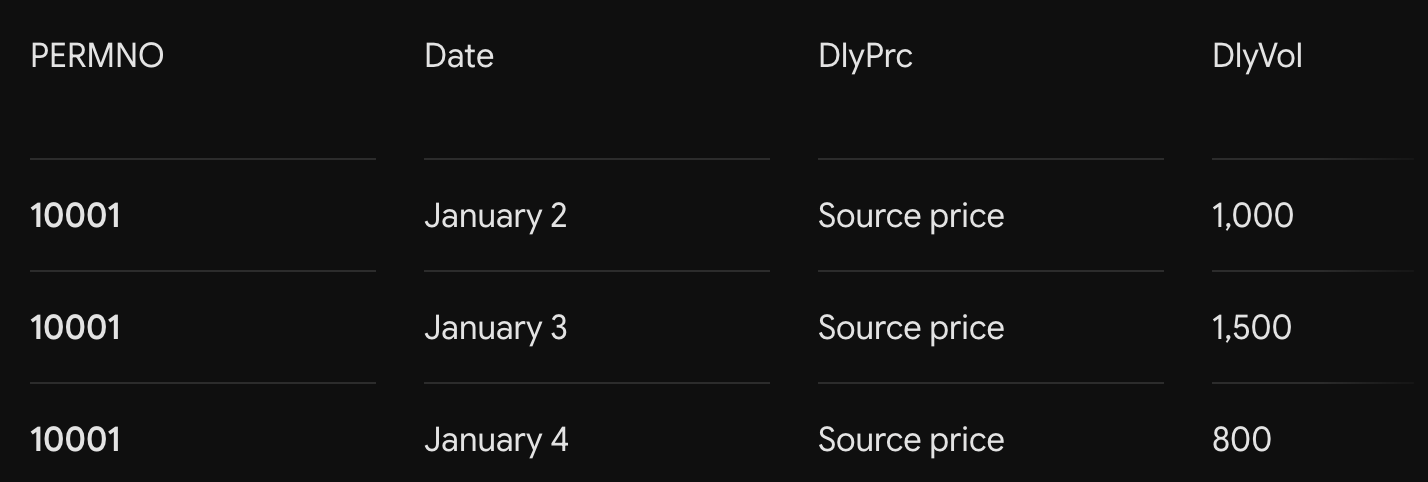
The adjustment module first produces an auditable adj_price and then a firm-local price_change. The daily-feature functions use those rows to create dollar_volume, signed_flow, and amihud_ratio. Under the configured zero-change convention, the unchanged observation contributes zero signed flow rather than being forced into a buy or sell direction. The upward and downward observations contribute signed volume with opposite directions.
All three rows receive the same calendar month key. If the firm has at least the configured minimum number of nonzero-volume days in the actual input, build_firm_month_features reduces the daily rows to one firm-month row. That row receives the sum of unsigned volume, the sample standard deviation of daily volume, and the sum of daily signed flow. The Amihud estimator uses only daily rows with valid returns and strictly positive dollar volume, so its valid-day count can differ from the count used for other features.
Later modules consume these columns differently. The panel regressions use the current firm-month volume features to explain either the current return or the same firm’s next calendar-month return. The lambda-return regressions use one current-month lambda column at a time. Forecasting uses the available current information inside an expanding chronological window. Portfolio formation ranks on a configured current-information signal and only then associates the resulting portfolios with subsequent returns.
This example explains data shapes and timing; it is not a paper calibration, an executed calculation, or a reproduced result.
Evidence-preserving interpretation
The paper contains unresolved contradictions that the pipeline should preserve rather than harmonize silently. Its theoretical discussion gives inconsistent comparative-static descriptions involving noise-trading variance and lambda. Its narrative expectations for signed-flow coefficients do not always agree with reported one-month-ahead coefficient signs. Section and table references are also inconsistent in the supplied extraction.
These issues affect interpretation, but they do not justify changing observed or reported signs in code. Result tables should retain specification labels, estimator names, sample counts, and provenance so that differences can be inspected directly.
The same principle applies to damaged equations. No formula is reconstructed when the supplied canonical record is incomplete or OCR-damaged. The implementation can document a prose-defined behavior or expose an explicit configuration choice, but it should not present an inferred formula as though it came from the paper.
Finally, all verification flags are disabled under the run policy. Static verification, semantic code verification, execution, test generation, and final quality review were not performed. The planned invariants—unique firm-month keys, same-firm target alignment, finite denominators, nondecreasing forecast windows, and separation of paper targets from computed outputs—are useful design requirements, not checks claimed to have passed.
Local data contracts and preprocessing decisions
Before estimating liquidity or return predictability, which observations should count as comparable trading records? The reproduction answers that question with a data contract: an explicit agreement about column names, types, keys, filters, missing values, and external inputs. Configuration keeps uncertain choices visible instead of burying them inside preprocessing functions.
The paper’s empirical sample is based on CRSP daily equity data, with a stated main period of 2020–2025 and a default exchange filter for CRSP exchange codes 1, 2, and 3. The pipeline then creates monthly firm observations. These are paper-supported design elements. By contrast, the exact application of CRSP adjustment factors, return conventions, delisting-return treatment, winsorization scope, and inference settings is not fully specified. Those choices must remain configurable.
Required local inputs
The normalized daily table has one row for one PERMNO on one trading date. PERMNO is the CRSP firm identifier, and the daily uniqueness key is the pair (PERMNO, date). The required source fields are:
PERMNO: firm identifier.date: trading date.EXCHCD: CRSP exchange code.DlyPrc: daily price.DlyVol: daily share volume.DlyRet: daily stock return.ShrOut: shares outstanding.DisFacPr: CRSP price-adjustment field.DisFacShr: CRSP share-adjustment field.
DlyBid and DlyAsk may also be retained when available, but the core volume and lambda constructions do not require them.
The monthly inputs use a different key. Firm-level monthly returns and controls use (PERMNO, month), where month is normalized to a calendar-month timestamp. Aggregate risk-free data use month alone. The paper also identifies H.15 Treasury-bill data, WRDS book-to-market and factor data, and possible delisting and point-in-time membership information for particular analyses. These files are external requirements; they cannot be inferred from CRSP daily rows or fabricated by the loader.
The daily loader is local-only. Its public responsibility is to read a supported file, normalize types and dates, preserve source fields, sort chronologically, and reject duplicate firm-date observations. A focused excerpt shows the boundary check:
def validate_crsp_daily_columns(
    frame: pd.DataFrame, columns: DataColumnConfig
) -> None:
    """Validate the normalized CRSP daily schema and key invariants.

    The required schema contains PERMNO, date, EXCHCD, DlyPrc, DlyVol, DlyRet,
    ShrOut, DisFacPr, and DisFacShr under the names in ``columns``.  Bid and ask
    are deliberately optional because the paper identifies them as optional
    inputs and the core feature pipeline does not require them.
    """
    required = columns.required_daily_columns()
    missing = [name for name in required if name not in frame.columns]
    if missing:
        raise ValueError(f"CRSP daily frame is missing required columns: {missing}")

    if not isinstance(frame.index, pd.RangeIndex):
        # Index type is not part of the data contract; reset-indexed input is
        # normalized by the loader, while direct callers receive a clear error.
        if frame.index.has_duplicates:
            raise ValueError("CRSP daily frame index must not contain duplicates")

    if frame[columns.permno].isna().any():
        raise ValueError("PERMNO contains missing values")
    if frame[columns.date].isna().any():
        raise ValueError("date contains missing values")

    permno = pd.to_numeric(frame[columns.permno], errors="coerce")
    if permno.isna().any() or ((permno % 1) != 0).any():
        raise ValueError("PERMNO must contain integer-like values")
    if not pd.api.types.is_datetime64_any_dtype(frame[columns.date]):
        raise TypeError("date must be datetime-like after normalization")

    duplicate_keys = frame.duplicated(
        subset=[columns.permno, columns.date], keep=False
    )
    if bool(duplicate_keys.any()):
        raise ValueError("CRSP daily input contains duplicate PERMNO-date observations")
validate_crsp_daily_columns receives a pandas DataFrame and a DataColumnConfig. Its output is None when the schema is acceptable; malformed schemas raise an exception rather than silently dropping or repairing fields. The loader itself returns a table with one normalized row per firm-date observation. It does not establish that the source data have the same point-in-time or corporate-action treatment as the paper.
Configuration makes ambiguity explicit
DataColumnConfig maps source names to the fields used downstream. ReproductionConfig stores sample dates, local paths, filters, adjustment conventions, winsorization, covariance, forecasting, and portfolio choices. The following is a compact local configuration example copied from the generated tutorial:
from pathlib import Path

from liquidity_premium.config import ReproductionConfig

config = ReproductionConfig(
    sample_start="2020-01-01",
    sample_end="2025-12-31",
    daily_path=Path("data/crsp_daily.parquet"),
    monthly_returns_path=Path("data/monthly_returns.parquet"),
    risk_free_path=Path("data/risk_free_rates.csv"),
    auxiliary_monthly_path=Path("data/auxiliary_monthly.parquet"),
    output_dir=Path("outputs"),
)
The defaults additionally specify exchange codes (1, 2, 3), a minimum of 15 nonzero-volume days, the price_only adjustment convention, monthly winsorization, an uncentered lambda estimator, equal-weighted deciles, and no fixed Newey–West lag unless one is supplied. These are not all paper facts. The period, exchange codes, and 15-day rule are supported by the supplied paper description; the adjustment, winsorization, covariance, and portfolio defaults resolve underspecified choices in the implementation.
For example, a run can make those choices more visible:
config = ReproductionConfig(
    sample_start="2020-01-01",
    sample_end="2025-12-31",
    daily_path=Path("data/crsp_daily.parquet"),
    monthly_returns_path=Path("data/monthly_returns.parquet"),
    risk_free_path=Path("data/risk_free_rates.csv"),
    auxiliary_monthly_path=Path("data/auxiliary_monthly.parquet"),
    adjustment_convention="price_only",
    winsorization_scope="month",
    newey_west_lags=4,
    portfolio_weighting="equal",
)
The value 4 here is an implementation example, not a lag length specified by the paper. The paper does not provide an exact Newey–West lag. Similarly, price_only is a selected convention, not a uniquely established interpretation of DisFacPr and DisFacShr.
Filter order and the 15-day rule
The intended order is to load and normalize the daily data, restrict the sample period and exchanges, construct the calendar-month key, and apply the minimum-volume-day rule before aggregation. The paper’s default exchange filter retains codes 1, 2, and 3. The minimum-volume filter retains a firm-month when it contains at least 15 finite, strictly positive DlyVol observations.
The generated filter is deliberately a row filter: it returns the daily observations belonging to qualifying groups, leaving aggregation to a later module.
def filter_minimum_volume_days(
    frame: pd.DataFrame,
    minimum_days: int = 15,
) -> pd.DataFrame:
    """Retain firm-month groups with enough nonzero-volume trading days.

    A qualifying day has finite, strictly positive ``DlyVol``.  The count is
    computed independently for each ``PERMNO`` and calendar month, matching
    the paper's minimum-15-nonzero-volume-day filter.  This function is
    deliberately a row filter: aggregation and feature construction occur in
    the downstream aggregation module.  The original columns and row order
    are preserved for surviving observations.
    """
    _require_columns(frame, ("PERMNO", "date", "DlyVol"))
    if not isinstance(minimum_days, int) or isinstance(minimum_days, bool):
        raise TypeError("minimum_days must be an integer")
    if minimum_days < 1:
        raise ValueError("minimum_days must be positive")

    dates = _coerce_dates(frame["date"], "date")
    volume = pd.to_numeric(frame["DlyVol"], errors="coerce")
    valid_volume = volume.notna() & volume.gt(0) & volume.ne(float("inf")) & volume.ne(float("-inf"))

    month_key = dates.dt.to_period("M")
    group_keys = pd.DataFrame(
        {"PERMNO": frame["PERMNO"], "_month": month_key},
        index=frame.index,
    )
    counts = valid_volume.groupby([group_keys["PERMNO"], group_keys["_month"]], dropna=False).sum()
    row_counts = pd.MultiIndex.from_arrays(
        [group_keys["PERMNO"], group_keys["_month"]],
        names=["PERMNO", "_month"],
    )
    qualifying = counts.ge(minimum_days)
    mask = qualifying.reindex(row_counts, fill_value=False).to_numpy()
    return frame.loc[mask].copy()
The function accepts a daily DataFrame and returns a same-column DataFrame containing only rows from qualifying firm-month groups. It does not create a monthly row or calculate a return. A group with missing, infinite, or zero volume does not count that observation toward the threshold. The resulting aggregation must later enforce uniqueness of (PERMNO, month).
Adjustment fields and return conventions
The paper requires split-adjusted prices and names DisFacPr and DisFacShr, but the supplied extraction does not give an unambiguous formula for applying both fields. The generated compute_adjusted_price function therefore exposes three conventions: raw, price_only, and price_and_shares. It preserves the raw adjustment columns instead of overwriting them.
This distinction matters because adjusted prices feed later price changes, signed-flow directions, and potentially dollar-volume calculations. The selected convention can change derived variables, so it belongs in configuration and provenance.
validate_adjustment_factors checks that the adjustment fields exist and are finite and strictly positive under a factor-based convention. compute_adjusted_price returns a float-compatible series aligned with the input rows. Invalid adjusted prices raise an error rather than becoming silently usable values. These checks constrain the input but do not prove that a chosen convention matches CRSP documentation or the paper’s intended processing.
Monthly returns require a separate decision. load_monthly_returns normalizes the firm-month key and exposes a recognized return field as StockRet, but it does not automatically combine delisting returns or convert raw returns to excess returns. load_risk_free_rates normalizes aggregate monthly rates as risk_free_rate, but does not convert annualized yields to monthly returns. Those transformations depend on source units and conventions that the paper does not state consistently across all analyses.
This separation prevents a raw return, a delisting-adjusted return, and an excess return from being treated as interchangeable. Each model input should identify which convention it uses.
Monthly auxiliary data and duplicate protection
The monthly loaders normalize date-like values to month-start timestamps. Thus, dates within the same calendar month map to the same month key. Firm-month auxiliary data must not contain duplicate (PERMNO, month) rows, while aggregate risk-free data must not contain duplicate month rows. Duplicate keys are rejected rather than silently aggregated, because silent aggregation could conceal a data join error.
The loaders preserve auxiliary columns such as book-to-market or factor returns. They do not invent unavailable values. If WRDS factors, H.15 rates, point-in-time membership, or delisting returns are absent, the corresponding analysis must either be omitted or run with an explicitly documented reduced input set.
Provenance without fabricated evidence
A provenance record documents the configuration and local input paths. It does not claim that the files exist, that they are complete, or that they reproduce the paper’s reported coverage. The generated export function makes this boundary explicit:
def write_provenance(
    path: Path,
    config: ReproductionConfig,
    inputs: list[Path],
) -> None:
    """Write configuration and local input-path metadata for a reproduction run.

    The provenance record documents choices that affect reproducibility, including
    adjustment, winsorization, covariance, forecast, and portfolio conventions.
    It records paths only; it does not assert that external CRSP, H.15, WRDS, or
    delisting data are present, complete, or sufficient to reproduce paper results.
    """
    if not isinstance(config, ReproductionConfig):
        raise TypeError("config must be a ReproductionConfig")
    if not isinstance(inputs, list):
        raise TypeError("inputs must be a list of pathlib.Path values")
    if any(not isinstance(input_path, Path) for input_path in inputs):
        raise TypeError("each input must be a pathlib.Path")

    payload: dict[str, object] = {
        "schema_version": "1.0",
        "record_type": "liquidity_premium_reproduction_provenance",
        "paper_id": "2607.01377v1",
        "paper_title": "Liquidity Premium and Investment Horizons",
        "configuration": asdict(config),
        "input_paths": [str(input_path) for input_path in inputs],
        "notes": [
            "This record describes a local reproduction configuration and does not contain computed results.",
            "External data availability, preprocessing conventions, and unspecified paper choices affect reproducibility.",
            "Paper-reported targets are not represented as independently reproduced values.",
        ],
    }
    write_json(payload, path)
write_provenance receives a configuration and a list of local Path objects and writes metadata through write_json. The important invariant is evidentiary: a paper target, such as the reported firm or firm-month count, must remain a comparison target and must never be inserted into a computed report merely because it is known from the paper.
Worked example: one firm and two keys
Consider a conceptual daily input for one firm, PERMNO=10001, on several dates in January 2020. Each row has DlyPrc, DlyVol, DlyRet, ShrOut, DisFacPr, and DisFacShr, plus EXCHCD=1. After date normalization, all rows receive the same calendar month key, 2020-01-01. The daily key is therefore (10001, date), while the eventual aggregate key is (10001, 2020-01-01).
If one row has missing volume, it does not count toward the 15-day threshold. If a row has zero volume, it also does not count. If the firm has fewer than 15 finite, strictly positive-volume days in January, every January row is removed by filter_minimum_volume_days; no partial firm-month is created. With at least 15 qualifying days, the later aggregation can produce exactly one January row for PERMNO=10001.
The later pipeline assigns responsibilities as follows:
load_crsp_dailyvalidates and sorts the source rows.filter_exchange_codesremoves observations outside codes 1, 2, and 3.filter_sample_periodapplies inclusive sample-date bounds.compute_adjusted_pricecreates an audit-preserving adjusted-price series under the configured convention.Daily feature functions use the adjusted prices, volumes, and returns to create derived columns.
The aggregation module converts qualifying daily rows into one firm-month row.
Monthly loaders and alignment functions attach returns and controls without crossing firm boundaries.
This example explains keys, timing, and responsibilities only. It is not a CRSP result, and no generated code or numerical output is claimed to have been executed.
What a full reproduction still needs
A complete numerical reproduction depends on local CRSP data and, for relevant specifications, H.15, WRDS, factor, point-in-time, and delisting inputs. It also requires explicit choices for:
application of
DisFacPrandDisFacShr;raw, delisting-adjusted, or excess-return conventions;
winsorization scope and timing;
covariance and standard-error treatment;
handling of missing calendar months and external controls;
portfolio and risk-free-rate conventions.
The paper’s reported coverage and summary values remain paper claims until a run with suitable data produces comparable outputs. Under the authoritative run policy, execution, static verification, semantic code verification, and numerical validation were not performed. The implementation therefore documents a reproducible boundary and a set of explicit decisions, not a completed empirical match.
3. From daily prices and volume to firm-month features
How does a table of daily CRSP observations become the monthly predictors used in the paper? The pipeline first creates row-level quantities—adjusted price, price change, dollar volume, signed flow, and an Amihud ratio—and then compresses those rows into one record per PERMNO and calendar month.
Unsigned volume measures how many shares traded. Signed flow preserves a direction: the same volume contributes positively after an upward price change and negatively after a downward change. An unchanged price contributes zero under the implementation convention. The Amihud-style ratio instead measures absolute return per dollar traded, so a zero-dollar-volume observation has no valid ratio.
Daily inputs and shape flow
The normalized daily frame contains one row per security-date observation. The relevant columns are PERMNO, date, DlyPrc, DlyVol, and DlyRet; DisFacPr and DisFacShr provide the adjustment fields named by the paper. The daily feature functions preserve the input index and add derived columns without changing the number of daily rows.
The intended shape transition is:
daily source table:
(n_daily_rows, n_columns);daily feature table:
(n_daily_rows, n_columns + derived_columns);firm-month table: one row for each retained
(PERMNO, month)key.
make_month_key converts each parseable date to a pandas monthly Period. The aggregation key is therefore the pair PERMNO and month, not merely the calendar month. This prevents observations from different firms being combined.
Adjusted prices and daily dollar volume
The paper names CRSP adjustment fields but does not uniquely specify how DisFacPr and DisFacShr should be applied. compute_adjusted_price therefore exposes explicit conventions such as raw, price_only, and price_and_shares. The selected convention is an implementation decision and should be recorded in configuration and provenance; it is not a paper fact. Raw source columns remain available for auditability.
compute_daily_price_change calculates chronological differences within each PERMNO. A missing prior price produces a missing change. The daily dollar-volume function then prefers the derived adj_price column and multiplies it by DlyVol. Share volume must be finite and nonnegative. Missing inputs remain missing rather than being converted into artificial values.
A focused excerpt shows the dollar-volume boundary:
def compute_daily_dollar_volume(frame: pd.DataFrame) -> pd.Series:
    """Compute daily dollar volume as price times share volume.

    The function uses ``adj_price`` when it is already present, because the
    preprocessing pipeline constructs price-based features from the selected
    split-adjusted price.  Otherwise it falls back to ``DlyPrc`` and uses its
    absolute value, matching CRSP's convention that a negative price can mark
    a bid/ask-related observation.  This fallback is an implementation
    decision; the supplied paper does not fully specify the adjustment-factor
    convention.
    """
    if not isinstance(frame, pd.DataFrame):
        raise TypeError("frame must be a pandas DataFrame")

    price_column = (
        _ADJUSTED_PRICE_COLUMN
        if _ADJUSTED_PRICE_COLUMN in frame.columns
        else _DEFAULT_PRICE_COLUMN
    )
    if price_column not in frame.columns:
        raise KeyError(
            f"Missing price column: expected {price_column!r} or "
            f"{_ADJUSTED_PRICE_COLUMN!r}"
        )
    if _DEFAULT_VOLUME_COLUMN not in frame.columns:
        raise KeyError(f"Missing share-volume column: {_DEFAULT_VOLUME_COLUMN!r}")

    price = _numeric_series(frame[price_column], price_column).abs()
    volume = _numeric_series(frame[_DEFAULT_VOLUME_COLUMN], _DEFAULT_VOLUME_COLUMN)
    invalid_volume = volume.notna() & (~np.isfinite(volume) | (volume < 0))
    if bool(invalid_volume.any()):
        raise ValueError("Share volume must be finite and nonnegative when present")

    dollar_volume = (price * volume).astype("float64")
    dollar_volume.name = "dollar_volume"
    finite = dollar_volume.notna() & np.isfinite(dollar_volume)
    dollar_volume.loc[dollar_volume.notna() & ~finite] = np.nan
    return dollar_volume.reindex(frame.index)
The important implementation invariant is that the returned dollar_volume is aligned row-for-row with the input. It is nonnegative when present, but it can be missing when price or share volume is unavailable.
Signed order flow
The paper’s monthly signed-flow construction begins with daily share volume and the direction of the split-adjusted price change. Its purpose is to create an observable proxy for directional order flow before aggregation. The supplied canonical expression is:
Here, i identifies the firm and t identifies the month. τ indexes trading days within that month. Volume_iτ is daily share volume, while ΔP_iτ is the split-adjusted daily price change. The sign function maps a positive change to 1, a negative change to -1, and an unchanged change to 0 under this implementation convention. The result, signedflow_it, is one signed scalar for the firm-month.
The code separates this operation into a daily function and a monthly aggregation. The daily function implements the direction step:
def compute_daily_signed_flow(
    volume: pd.Series, price_change: pd.Series
) -> pd.Series:
    """Compute daily signed order flow from share volume and price direction.

    This implements Eq. 9: daily volume is multiplied by the sign of the
    split-adjusted daily price change.  An unchanged price has sign zero, so
    its signed flow is exactly zero.  Missing volume or price change remains
    missing rather than being treated as a trading direction.
    """
    volume_values = _numeric_series(volume, "volume")
    change_values = _numeric_series(price_change, "price_change")
    if not volume_values.index.equals(change_values.index):
        raise ValueError("volume and price_change must have identical indexes")

    invalid_volume = volume_values.notna() & (
        ~np.isfinite(volume_values) | (volume_values < 0)
    )
    if bool(invalid_volume.any()):
        raise ValueError("volume must be finite and nonnegative when present")

    # Eq. 9: signed flow uses volume times the sign of the price change.
    direction = np.sign(change_values)
    signed_flow = (volume_values * direction).astype("float64")
    signed_flow.name = "signed_flow"
    signed_flow.loc[change_values.isna() | volume_values.isna()] = np.nan
    finite = signed_flow.notna() & np.isfinite(signed_flow)
    if bool((signed_flow.notna() & ~finite).any()):
        raise ValueError("signed flow contains non-finite values")
    return signed_flow.reindex(volume.index)
The function accepts two one-dimensional, identically indexed series. It returns another one-dimensional series of the same length. A missing price change is not interpreted as a sell direction; the corresponding signed flow is missing. This preserves a distinction between no directional movement, represented by zero, and unavailable information, represented by missingness.
Monthly total volume and dispersion
The paper defines monthly unsigned share volume as follows:
sumvolume_it is the nonnegative total share volume for firm i in month t. In aggregate_monthly_volume, it is computed from valid daily DlyVol values and returned as the sumvolume field. The function also returns nonzero_volume_days, which records the activity count used by the minimum-activity filter.
The paper uses within-month volume standard deviation as a proxy for noise-trading variation. The canonical LaTeX for equation 8 is unavailable in the supplied extraction, so it is not displayed or reconstructed here. The implementation follows the paper’s prose description and uses the sample standard deviation, equivalent to pandas ddof=1, over valid daily volume observations. This is a prose-derived implementation detail, not a transcription of missing equation LaTeX.
The minimum-volume rule retains only firm-month groups with at least 15 strictly positive-volume trading days. The filter is applied at the group level before aggregation, so all daily rows from a nonqualifying group are removed. The 15-day rule normally supplies enough observations for a numeric sample standard deviation, although missing values are still handled explicitly.
The aggregation function then produces one record per firm-month:
# Eq. 7: monthly total unsigned share volume.
total_volume = float(valid_volume.sum())

# Eq. 8: sample standard deviation of daily volume; canonical LaTeX is
# unavailable, so the documented ddof=1 convention is used.
stdvolume = float(valid_volume.std(ddof=1)) if len(valid_volume) >= 2 else np.nan

# Eq. 9: monthly signed order flow is the sum of daily signed flow.
signedflow = float(signed_flow.sum(min_count=1)) if signed_flow.notna().any() else np.nan
The resulting columns are sumvolume, nonzero_volume_days, stdvolume, and signedflow, with amihud_lambda added when daily Amihud ratios are supplied. build_firm_month_features sorts the output and rejects duplicate PERMNO-month keys.
Amihud-style illiquidity
The daily Amihud quantity measures absolute return per dollar traded. The paper’s monthly estimator is the mean of valid daily ratios:
In this expression, r_iτ is the daily stock return, DollarVolume_iτ is daily dollar trading volume, and n is the number of valid daily observations used in the average. i and t retain their firm and month meanings. The estimate is nonnegative when valid.
The daily implementation excludes rows with missing or non-finite returns and rows whose dollar-volume denominator is zero. It never turns division by zero into infinity. The valid daily ratios are then averaged within aggregate_monthly_volume as amihud_lambda.
Equation 15 gives the same estimator under the Method A label:
The superscript A identifies Method A, the Amihud-style level estimator. The symbols have the same meanings as in the preceding equation: n is the valid-day count, r_iτ is daily return, and DollarVolume_iτ is a positive daily denominator. In code, both equation records map to compute_daily_amihud_ratio followed by the within-month mean. The two equation labels describe the same calculation rather than two different daily algorithms.
A focused denominator check from the generated implementation is:
valid = (
    returns.notna()
    & np.isfinite(returns)
    & dollars.notna()
    & np.isfinite(dollars)
    & (dollars > 0)
)
ratio = pd.Series(np.nan, index=returns.index, dtype="float64", name="amihud_ratio")
ratio.loc[valid] = (returns.loc[valid].abs() / dollars.loc[valid]).astype("float64")
if bool((ratio.notna() & ~np.isfinite(ratio)).any()):
    raise ValueError("Amihud ratios must be finite when present")
return ratio
Thus, a zero-dollar-volume day does not contribute to the monthly mean. This can make the number of valid Amihud days smaller than the number of days used for volume aggregation.
Worked example: three daily observations
Consider one firm with three already adjusted daily observations. Suppose the share volumes are 100, 200, and 300, and the corresponding price changes are positive, zero, and negative. The signed contributions are therefore +100, 0, and -300; the unchanged price contributes exactly zero. The unsigned total volume is 600.
If the three valid daily volumes are used for the sample dispersion, the calculation is the sample standard deviation of 100, 200, and 300, using denominator n - 1 rather than n. This example is conceptual: the paper’s minimum filter requires at least 15 positive-volume days for a retained firm-month, so three rows alone would not survive the actual aggregation filter.
For the Amihud calculation, suppose the daily returns are 0.01, 0.02, and -0.03, and the corresponding positive dollar volumes are 1,000, 2,000, and 0. The first two ratios are valid. The third is excluded because its denominator is zero; it does not become an infinite ratio and is not included in n. The monthly Amihud value is consequently the mean of the valid ratios only.
The same fields would then flow into later stages as follows: sumvolume, stdvolume, signedflow, and amihud_lambda become firm-month predictors; StockRet is merged from monthly data; and the alignment stage creates a same-firm next-month target. No numerical result from this illustrative example is a paper result or a verified execution outcome.
Orchestration and evidence boundary
build_daily_audit_table exposes the cleaned daily frame with derived fields for inspection. build_empirical_panel calls the daily stage, aggregates firm-month features, constructs controls, estimates lambda values, merges monthly returns, and aligns next-month returns. The generated pipeline does not access a network; CRSP and auxiliary files must already exist locally.
The implementation enforces key structural constraints such as nonnegative volume, finite valid Amihud ratios, at least 15 positive-volume days in retained groups, and unique PERMNO-month rows. However, the supplied verification records state that static verification and semantic code verification were skipped under the run policy. These constraints describe intended implementation behavior, not checks claimed to have passed. The adjustment convention, exact corporate-action treatment, return and delisting conventions, and winsorization policy remain configuration-dependent.
The theoretical Kyle relations and their empirical interpretation
How can a price-impact coefficient connect trading activity to prices without being confused with a directly observed quantity? The paper’s Kyle-style model provides the intuition: an informed trader responds to a fundamental-value deviation, noise traders add orders that are not separately observed, and a market maker adjusts the transaction price according to total signed order flow. The empirical pipeline then uses observed signed volume as a proxy for this latent flow; it does not observe the theoretical informed and noise orders individually.
This section therefore has two layers. The first is a scalar theoretical API in src/liquidity_premium/models/kyle.py. The second is the empirical estimation workflow described elsewhere, where daily signed flow and price changes are used to estimate firm-month price impact. The theoretical functions accept scalar values and return scalar values. They are not fitted to CRSP data by the generated module.
Informed demand responds to a value discrepancy
In the single-period model, v is the asset’s liquidation value, while p_0 is its initial or prior price. Their difference represents the fundamental-value discrepancy available to the informed trader. The positive scalar beta measures informed-trading intensity. The paper expresses informed demand as follows:
This is eq_1. The symbol x is the informed trader’s scalar market order. If v exceeds p_0, the order is positive under this convention; if v is below p_0, it is negative. The restriction beta > 0 means that the intensity scales the direction implied by the value discrepancy rather than reversing it.
The generated function informed_order(v, p0, beta) implements this relation. It validates that the inputs are finite scalars and that beta is strictly positive, then returns the scalar order quantity. The validation is an implementation safeguard corresponding to the model’s stated positivity restriction; it does not estimate beta or infer v from market data.
A focused excerpt from src/liquidity_premium/models/kyle.py shows the mapping:
def informed_order(v: float, p0: float, beta: float) -> float:
    """Compute informed demand from the supplied single-period Kyle relation.

    Parameters
    ----------
    v:
        Asset liquidation value.
    p0:
        Initial or prior asset price.
    beta:
        Positive informed-trading intensity.

    Returns
    -------
    float
        Informed order quantity ``x``.  The sign follows ``v - p0``.

    Notes
    -----
    Implements eq. 1: ``x = beta (v - p0)``.  This is a theoretical
    calculation, not an estimator of empirical order flow.
    """
    liquidation_value = _validate_finite_scalar(v, "v")
    initial_price = _validate_finite_scalar(p0, "p0")
    intensity = _validate_positive_scalar(beta, "beta")

    # Eq. 1: informed demand is proportional to the liquidation-value deviation.
    return intensity * (liquidation_value - initial_price)
The final comment is important for reproduction fidelity: the function computes x from supplied scalar inputs, but it does not produce the empirical signedflow feature.
Aggregate flow is latent in the model
The theoretical informed order is only one component of total order flow. Let u denote a noise-trader order and let y denote aggregate signed order flow. In the model, aggregate flow is formed by adding the informed and noise components. The helper aggregate_order_flow(informed, noise) performs that addition and preserves the signs of both scalar inputs.
This distinction matters when reading the empirical pipeline. The model’s y is latent: the data do not separately identify x and u. By contrast, empirical signedflow is constructed from daily share volume and the sign of the observed split-adjusted price change. It is a proxy motivated by the theory, not an observed measurement of y, x, or u.
The market maker maps flow into price
The paper’s market-maker rule says that the transaction price equals the prior price plus a flow-dependent price adjustment. The coefficient lambda is the Kyle price-impact coefficient: it measures the price displacement associated with one unit of aggregate signed flow. The paper writes:
This is eq_2. Here, p is the transaction price, p_0 is the initial or prior price, y is aggregate theoretical flow, and lambda is a positive scalar. Because lambda is positive, positive aggregate flow raises the transaction price relative to p_0, while negative aggregate flow lowers it.
The generated market_maker_price(p0, lam, aggregate_flow) function implements this pricing rule. It checks that p0, lam, and the aggregate flow are finite and that lam is strictly positive. The function is a theoretical pricing helper, not an empirical regression. In particular, passing an observed signed-flow value to it would be an API illustration, not proof that the observed value is the model’s latent y.
The relevant implementation excerpt is:
def market_maker_price(p0: float, lam: float, aggregate_flow: float) -> float:
    """Apply the linear market-maker pricing rule to aggregate flow.

    Parameters
    ----------
    p0:
        Initial or prior asset price.
    lam:
        Positive Kyle price-impact coefficient.
    aggregate_flow:
        Aggregate signed order flow ``y``.

    Returns
    -------
    float
        Transaction price ``p``.

    Notes
    -----
    Implements eq. 2: ``p = p0 + lambda y``.  The positive-lambda validation
    ensures that positive (negative) flow produces a positive (negative) price
    displacement relative to ``p0``.
    """
    initial_price = _validate_finite_scalar(p0, "p0")
    price_impact = _validate_positive_scalar(lam, "lam")
    flow = _validate_finite_scalar(aggregate_flow, "aggregate_flow")

    # Eq. 2: the market maker maps aggregate signed flow into price impact.
    return initial_price + price_impact * flow
The empirical within-month regression uses the same conceptual direction—price change related to signed flow—but estimates a firm-month coefficient from daily observations. That later coefficient is an empirical construction whose exact scale and interpretation depend on the data adjustments, regression convention, and valid observations.
Sequential price changes
The sequential extension indexes trading rounds by n. In round n, Delta y_n is the order-flow innovation and lambda_n is the price-impact coefficient for that round. The resulting price innovation is:
This is eq_5. The scalar Delta p_n is the price change in round n; lambda_n is a positive, round-specific price-impact coefficient; and Delta y_n is the round’s signed order-flow innovation. The equation does not specify a full dynamic path for lambda_n; it only states how a given round’s coefficient maps that round’s flow innovation into a price change.
The generated sequential_price_change(lam_n, delta_y_n) function implements this multiplication. It validates positive lam_n and finite delta_y_n, then returns a scalar. Its sign invariant follows directly from the positivity restriction: a positive flow innovation produces a positive price change, a negative innovation produces a negative price change, and a zero innovation produces zero change.
def sequential_price_change(lam_n: float, delta_y_n: float) -> float:
    """Compute a sequential-auction price innovation.

    Parameters
    ----------
    lam_n:
        Positive price-impact coefficient for round ``n``.
    delta_y_n:
        Order-flow innovation in round ``n``.

    Returns
    -------
    float
        Round-specific price change ``Delta p_n``.  Its sign equals the sign of
        ``delta_y_n`` unless the innovation is zero.

    Notes
    -----
    Implements eq. 5: ``Delta p_n = lambda_n Delta y_n``.  No dynamic path for
    ``lambda_n`` is inferred or simulated here.
    """
    round_price_impact = _validate_positive_scalar(lam_n, "lam_n")
    flow_innovation = _validate_finite_scalar(delta_y_n, "delta_y_n")

    # Eq. 5: each round's price innovation scales that round's flow innovation.
    return round_price_impact * flow_innovation
Worked API illustration
Consider a hypothetical asset with v = 101.0, p0 = 100.0, and beta = 2.0. The informed-order function represents a value deviation of one price unit scaled by an intensity of two, so the conceptual informed order is positive. Suppose a noise trader submits a negative order; aggregate_order_flow adds that noise order to the informed order. A positive lam then maps the resulting signed flow into a transaction-price displacement.
For a sequential illustration, set lam_n to a positive value and delta_y_n to either a positive or negative flow innovation. The returned price change follows the innovation’s sign. These are hand-worked API examples for understanding scalar inputs, scalar outputs, and sign behavior. They are not CRSP observations, paper calibrations, or executed numerical results.
The planned tests in tests/test_theoretical_kyle.py mirror these direct relations for eq_1, eq_2, and eq_5. Under the run policy, those tests were not executed or verified; their presence describes intended coverage rather than a passed check.
What is deliberately excluded
The paper extraction does not provide safe canonical formulas for every theoretical statement. eq_3, the closed-form equilibrium values for beta and lambda, is OCR-damaged and is not reconstructed. eq_4 is a qualitative sequential comparative-static claim whose conditioning and distributional assumptions are underspecified, so it is not simulated. eq_6, concerning the continuous-time path of lambda(t), also has damaged canonical LaTeX and is not implemented.
These exclusions are deliberate evidence boundaries. The generated module implements only the supplied scalar relations eq_1, eq_2, and eq_5; it does not fill gaps by importing a familiar Kyle formula or by choosing an unstated dynamic model. The paper’s broader model description and its formal single-period presentation are also not fully reconciled, and its statements about how noise-trading variance affects price impact are internally inconsistent. Those comparative statics should remain documented ambiguities rather than being resolved silently in code.
Finally, the theoretical lambda should not be treated as identical to either empirical firm-month estimator. The empirical pipeline estimates price impact or illiquidity from observed daily price, return, volume, and signed-flow proxies. The theoretical functions explain why such a coefficient is economically meaningful; they do not identify it from the supplied scalar inputs or replace the empirical estimator.
Estimating firm-month lambda
How can several daily observations become one monthly measure of price impact? For each PERMNO and calendar month, the reproduction computes two separate scalars. Method B estimates how daily price changes respond to signed daily flow. Method A computes an Amihud-style average of absolute return per dollar traded. They address related notions of illiquidity, but they are not interchangeable columns.
The daily inputs for one firm-month are one-dimensional vectors with shape (n_days,): price_change contains split-adjusted daily price changes, signed_flow contains signed daily volume, return_ contains daily returns, and dollar_volume contains daily dollar trading volume. The grouped function reduces each valid group to one row containing regression_lambda, amihud_lambda, and estimator-specific valid-day counts.
Method B: price change on signed flow
The paper’s within-month regression relates daily price changes to daily signed order flow. Its displayed specification has no intercept, so the default implementation is an uncentered one-predictor regression.
Here, \Delta P_{i\tau} is the daily split-adjusted price change for firm i on trading day \tau; OF_{i\tau} is that day’s signed-flow proxy; and \hat{\lambda}_{it} is the estimated scalar price-impact slope for firm i in month t. The residual \eta_{i\tau} captures the part of the daily price change not explained by the signed-flow regressor. The regression is performed separately within each PERMNO-month group, so its input has shape (n_valid_days, 1) for the design matrix and (n_valid_days,) for the response. The returned lambda is one scalar.
The default include_intercept=False follows the displayed equation. The generated function exposes include_intercept=True as an explicit alternative because the paper does not clearly resolve whether the intramonth estimator itself should include an intercept. This choice is separate from whether a later return regression includes an intercept.
The core implementation delegates the one-predictor calculation to fit_ols:
    try:
        result = fit_ols(
            flow.reshape(-1, 1),
            prices,
            include_intercept=bool(include_intercept),
        )
    except ValueError:
        # A group-level estimator should preserve missingness for groups that
        # cannot support the requested OLS specification rather than aborting
        # an otherwise valid firm-month batch.
        return None

    coefficient_index = 1 if include_intercept else 0
    estimate = float(result.coefficients[coefficient_index])
    return estimate if np.isfinite(estimate) else None
The flow.reshape(-1, 1) expression makes the design explicitly two-dimensional, while prices remains a one-dimensional response. With an intercept, coefficient index 1 is the flow slope because the intercept occupies index 0; without one, index 0 is the only coefficient. fit_ols validates finite values, row counts, rank, and residual degrees of freedom. At the group level, an unsupported specification becomes None, preserving estimator-specific missingness rather than stopping all firm-month processing.
A group also returns None when its signed-flow vector has no usable magnitude or when there are too few observations for the selected design. This is important for a no-intercept regression: a zero-flow group cannot identify a meaningful price-impact slope. The paper’s broader sample rule retains firm-months with at least 15 nonzero-volume trading days, but it does not state a separate minimum specifically for the intramonth regression. The upstream filter and these estimator-level degeneracy checks therefore serve different purposes.
Method A: Amihud-style illiquidity
The second estimator converts each valid daily observation into an absolute-return-per-dollar-volume ratio and averages those ratios within the firm-month. The paper records this construction as follows.
In this equation, \hat{\lambda}^{\mathrm{Amihud}}_{it} is the nonnegative Amihud-style estimate for firm i and month t. The integer n is the number of valid daily observations used in the mean. r_{i\tau} is the daily stock return, and \mathrm{DollarVolume}_{i\tau} is daily dollar trading volume. The absolute-value operator makes the numerator nonnegative, while the denominator must be strictly positive.
The paper also labels the same construction Method A:
Equations eq_13 and eq_15 therefore map to the same generated function, estimate_amihud_lambda. The function excludes rows with nonpositive dollar volume, so a zero denominator does not create an infinite ratio. Negative dollar-volume inputs are rejected as invalid. A valid result is nonnegative provided at least one daily observation remains.
The focused implementation is:
def estimate_amihud_lambda(
    return_: np.ndarray,
    dollar_volume: np.ndarray,
) -> float | None:
    """Estimate the within-firm-month Amihud-style illiquidity measure.

    The inputs are paired daily vectors with shape ``(n_days,)``.  Observations
    with non-finite returns or non-positive dollar volume are excluded, since
    the denominator in eq. 13 and eq. 15 must be strictly positive.  The
    resulting estimate is nonnegative whenever at least one valid observation
    remains.
    """
    returns = _as_float_vector(return_, "return_")
    dollars = _as_float_vector(dollar_volume, "dollar_volume")
    if returns.size != dollars.size:
        raise ValueError(
            "return_ and dollar_volume must have equal lengths: "
            f"{returns.size} != {dollars.size}."
        )
    if bool((dollars < 0).any()):
        raise ValueError("dollar_volume must be nonnegative.")

    valid = np.isfinite(returns) & np.isfinite(dollars) & (dollars > 0.0)
    if not bool(valid.any()):
        return None

    # Eq. 13 and Eq. 15: lambda_hat = mean(|r| / DollarVolume).
    ratios = np.abs(returns[valid]) / dollars[valid]
    if not np.isfinite(ratios).all():
        return None
    estimate = float(np.mean(ratios, dtype=np.float64))
    if estimate < 0.0 or not np.isfinite(estimate):
        return None
    return estimate
Notice the distinction between invalid input and unavailable estimation. A negative dollar volume raises an error because it violates the data contract. A group with no positive dollar-volume observations returns None, because no valid Amihud mean can be formed. The function uses float64 accumulation for the within-group mean and returns a scalar float when the calculation is defined.
Grouped firm-month computation
estimate_firm_month_lambdas applies both estimators independently to every (PERMNO, month) group. It requires price_change and signed_flow, plus a daily return column named DlyRet, return, or return_, and a dollar_volume column. It sorts by firm and month, converts the daily columns to numeric arrays, computes separate validity masks, and records the two estimates and their valid-day counts.
A compact excerpt shows the separate paths:
        regression_valid = np.isfinite(price_values) & np.isfinite(flow_values)
        amihud_valid = (
            np.isfinite(return_values)
            & np.isfinite(dollar_values)
            & (dollar_values > 0.0)
        )
        regression_lambda = (
            estimate_regression_lambda(
                price_values[regression_valid],
                flow_values[regression_valid],
                include_intercept=bool(include_intercept),
            )
            if bool(regression_valid.any())
            else None
        )
        amihud_lambda = (
            estimate_amihud_lambda(
                return_values[amihud_valid],
                dollar_values[amihud_valid],
            )
            if bool(amihud_valid.any())
            else None
        )
The two masks need not select the same days. For example, a daily price change and signed flow may be available while the daily return is missing, or a return may be available while dollar volume is zero. Consequently, regression_valid_days and amihud_valid_days are reported separately. The output contract is one row per firm-month key, with missingness retained independently for regression_lambda and amihud_lambda.
Lambda and the subsequent return target
Estimating lambda is only the first step. The current-month estimate must be aligned with the same firm’s subsequent calendar-month return. The paper writes the return relationship as:
Here, \mathrm{StockRet}_{i,t+1} is firm i’s return in the month after the estimate; \hat{\lambda}_{it} is the current-month lambda; \alpha_i and \beta_i are regression coefficients in the paper’s notation; and \varepsilon_{i,t+1} is the residual. This equation describes a later return regression, not the daily lambda estimator itself.
The supplied paper uses firm subscripts on the coefficients but also describes pooled observations and tables. The generated reproduction therefore treats pooled versus firm-specific estimation as an explicit modeling issue rather than assuming that the notation settles it. The alignment module uses an explicit PERMNO and month-plus-one join, so a missing calendar month does not silently become an adjacent observation.
    result["next_month"] = result[_MONTH] + pd.DateOffset(months=1)

    lookup = result[[_PERMNO, _MONTH, return_column]].rename(
        columns={_MONTH: "_target_month", return_column: "next_month_return"}
    )
    aligned = result.merge(
        lookup,
        left_on=[_PERMNO, "next_month"],
        right_on=[_PERMNO, "_target_month"],
        how="left",
        sort=False,
        validate="one_to_one",
    ).drop(columns=["_target_month"])
The join preserves the same firm identifier and requests exactly one calendar month later. The resulting next_month_return is then available to a later pooled regression; it is not used when computing the current-month lambda.
Worked example: vector contracts
Consider a synthetic firm-month with four daily observations. The intended inputs have these shapes:
price_change:(4,)signed_flow:(4,)return_:(4,)dollar_volume:(4,)
A caller can request both estimators through the public functions:
import importlib
import numpy as np

lambda_module = importlib.import_module(
    "liquidity_premium.estimators.lambda"
)

price_change = np.array([0.10, -0.04, 0.08, 0.02], dtype=float)
signed_flow = np.array([100.0, -50.0, 75.0, 25.0], dtype=float)
daily_return = np.array([0.010, -0.004, 0.008, 0.002], dtype=float)
dollar_volume = np.array(
    [10_000.0, 8_000.0, 12_000.0, 9_000.0],
    dtype=float,
)

regression_lambda = lambda_module.estimate_regression_lambda(
    price_change,
    signed_flow,
    include_intercept=False,
)
amihud_lambda = lambda_module.estimate_amihud_lambda(
    daily_return,
    dollar_volume,
)
This excerpt documents the API and shape transition only; it was not executed under the run policy, so no numerical output is claimed. The first result is a scalar regression slope, and the second is a scalar mean ratio. If the same firm-month supplied a zero vector for signed_flow, the regression estimator would return None because the no-intercept slope is degenerate. The Amihud estimator could still be valid if its return and positive dollar-volume vectors remained usable.
Method B’s incomplete source equation
The paper describes Method B as the slope from regressing daily price changes on daily volume multiplied by the sign of the daily price change. The generated code maps that prose to the same signed-flow regression path used for eq_12. However, the canonical LaTeX for eq_16 is OCR-truncated. No missing formula, intercept convention, or additional term is reconstructed here. The implementation follows only the supplied prose and the complete displayed relationship in eq_12.
Finally, do not conflate two independent choices: include_intercept on estimate_regression_lambda controls the intramonth price-impact estimator, while include_intercept on the later lambda-return regression controls the return model. The paper’s estimator ambiguity is therefore isolated in the API rather than silently propagated to every downstream specification.
Contemporaneous, predictive, and lambda-return regressions
How should a monthly activity measure be connected to a stock return without accidentally using the wrong firm or the wrong month? The reproduction treats every regression row as a keyed observation: PERMNO identifies the firm, month identifies the predictor month, and the target is either that same row’s return or the same firm’s return in the immediately following calendar month.
This section covers three related specifications. The first asks whether monthly volume features are associated with contemporaneous returns. The second uses those features to forecast the next month’s return. The third replaces the volume features with one firm-month lambda estimate at a time. All three are pooled ordinary least squares (OLS) regressions: observations from eligible firms and months enter one design matrix. The implementation does not constrain coefficient signs.
The common panel contract
The panel functions expect one row per PERMNO-month key. The base predictor columns are:
sumvolume: total unsigned share volume during the month;stdvolume: within-month sample standard deviation of daily volume;signedflow: monthly signed-flow proxy.
The target column is StockRet for the contemporaneous specification. For a one-month-ahead specification, the code creates next_month_return by matching the current firm and the next calendar month. Optional controls are appended by name. The paper discusses controls such as log market capitalization, book-to-market, momentum, and Amihud illiquidity, but unavailable external controls must remain missing rather than being fabricated.
The design-building function returns a predictor matrix with shape (n_used_observations, p), a target vector with shape (n_used_observations,), and labels preserving predictor order. The shared fit_ols function then optionally prepends an intercept column. With three base predictors and an intercept, the coefficient vector has shape (4,). The residual vector has length n_used_observations.
Equation 10: contemporaneous activity and returns
The contemporaneous specification asks whether firm-month activity and the return in that same firm-month are related. The paper records it as follows.
Here, StockRet_it is the monthly stock return for firm i in month t. The three predictors are total volume sumvolume_it, volume volatility stdvolume_it, and signed flow signedflow_it. alpha is the pooled regression intercept; beta_1, beta_2, and beta_3 are the corresponding slopes; and epsilon_it is the residual for that firm-month observation.
In the generated implementation, run_panel_return_regression selects this equation with horizon="contemporaneous". It delegates row construction to build_panel_dataset, creates the ordered predictor list, and passes the resulting arrays to build_panel_design and then fit_ols with an intercept.
A focused call is:
from liquidity_premium.regressions.panel import run_panel_return_regression

result = run_panel_return_regression(
    panel,
    horizon="contemporaneous",
    controls=None,
)
The no-control design has columns in this order:
sumvolume, stdvolume, signedflowThe returned labels add the specification context, including contemporaneous.no_controls.intercept. Rows with a missing target or missing required predictor are removed before fitting. The OLS primitive requires finite values, more observations than fitted parameters, and a full-rank design. These are numerical input conditions, not economic assumptions.
The paper does not fully specify fixed effects, weighting, clustering, or panel covariance treatment. The generated panel module therefore exposes a covariance argument but currently uses the shared classical homoskedastic OLS inference. That implementation choice must be recorded in result metadata and must not be presented as uniquely determined by the paper.
Equation 11: exact one-month-ahead alignment
The predictive version uses month-t activity to explain the same firm’s return in month t+1.
The notation changes only the target timing: StockRet_i,t+1 is the next calendar month’s return for the same firm. The predictors remain sumvolume_it, stdvolume_it, and signedflow_it, all measured in month t. alpha and the three beta coefficients retain their regression roles, while epsilon_i,t+1 is the forecast-regression residual.
The important implementation detail is that “next month” means an explicit calendar key, not merely the next available row for a firm. align_next_month_return normalizes month values, sorts by PERMNO and month, creates a month-plus-one key, and joins the return lookup on both PERMNO and target month. Thus, a January observation with no February row does not receive a March return as its target.
The core alignment operation is represented by this generated code excerpt:
result["next_month"] = result[_MONTH] + pd.DateOffset(months=1)

lookup = result[[_PERMNO, _MONTH, return_column]].rename(
    columns={_MONTH: "_target_month", return_column: "next_month_return"}
)
aligned = result.merge(
    lookup,
    left_on=[_PERMNO, "next_month"],
    right_on=[_PERMNO, "_target_month"],
    how="left",
    sort=False,
    validate="one_to_one",
).drop(columns=["_target_month"])
_PERMNO and _MONTH are the firm and calendar-month key columns. The lookup contains one return per firm-month. The one_to_one validation expresses the uniqueness contract, while the two-key merge prevents cross-firm leakage. Missing next-month observations remain missing and are later removed when build_panel_dataset prepares complete regression rows.
The predictive call changes only the horizon argument:
next_month_result = run_panel_return_regression(
    panel,
    horizon="next_month",
    controls=None,
)
With three base predictors and an intercept, this again produces four coefficients, but the retained observation count can be smaller because firms’ final available months have no following calendar-month target. The generated tests describe this behavior for synthetic panels, but those tests were not executed under the current run policy.
Adding controls without hiding missing data
Controls are appended after the three base predictors. For example, a fully populated controlled specification can be requested with:
controlled_result = run_panel_return_regression(
    panel,
    horizon="next_month",
    controls=[
        "log_size",
        "book_to_market",
        "momentum",
        "amihud_lambda",
    ],
)
If all four columns are available and numeric, the design contains seven economic predictors plus an intercept. The names must already exist in panel; the regression function raises an error for a missing requested column rather than inventing a substitute. This matters especially for book-to-market and factor-related inputs, which depend on external WRDS or factor files not supplied in the paper context.
The implementation keeps predictor units unstandardized. The paper does not specify a scaling convention, so raw economic units are retained for coefficient reporting. Every result should identify whether it uses no controls or controls and whether its return is raw, delisting-adjusted, or excess, because the supplied paper uses return conventions in different contexts without fully resolving them.
Equation 14: lambda as the sole predictor
The lambda-return specification tests whether a current firm-month illiquidity estimate predicts the same firm’s next-month return.
StockRet_i,t+1 is the next-month return for firm i. The predictor hat(lambda)_it is the lambda estimate formed from firm i’s daily observations in month t; it may be the regression-based estimator or the Amihud-style estimator. alpha_i and beta_i are the intercept and slope notation used in the paper, and epsilon_i,t+1 is the residual.
The generated implementation uses a pooled interpretation by default. Although the equation uses firm-specific subscripts on the coefficients, the supplied descriptions and reported pooled observation structure support fitting one regression over the eligible firm-month rows rather than silently fitting a separate regression per firm.
The lambda-return function recomputes same-firm next-month alignment through align_next_month_return, selects exactly one estimator column, removes rows with missing or non-finite estimator or target values, and calls fit_ols. A focused example is:
from liquidity_premium.regressions.lambda_return import (
    run_lambda_return_regression,
)

regression_lambda_with_intercept = run_lambda_return_regression(
    panel,
    estimator="regression_lambda",
    include_intercept=True,
)

amihud_lambda_uncentered = run_lambda_return_regression(
    panel,
    estimator="amihud_lambda",
    include_intercept=False,
)
The include_intercept argument belongs to this return regression. It is separate from the convention used earlier when estimating the firm-month regression lambda from daily price changes and signed flow. The generated default for that daily estimator is uncentered because the displayed price-impact equation omits an intercept; the return regression deliberately exposes both alternatives.
With an intercept, the lambda predictor matrix supplied to fit_ols has shape (n_used_observations, 1), and the fitted coefficient vector has shape (2,): intercept and lambda slope. Without an intercept, the coefficient vector has shape (1,) and contains only the lambda slope. The generated test specifies these structural dimensions without asserting any expected economic sign.
Comparing estimator and intercept specifications
The paper emphasizes that direct lambda-return relationships can be sensitive to both estimator construction and intercept treatment. run_lambda_specification_grid makes those comparisons explicit:
from liquidity_premium.regressions.lambda_return import (
    run_lambda_specification_grid,
)

lambda_grid = run_lambda_specification_grid(panel)
The grid contains four combinations:
regression_lambda, with intercept
regression_lambda, uncentered
amihud_lambda, with intercept
amihud_lambda, uncentered
Each row stores estimator and intercept labels, coefficient arrays, standard errors, t-statistics, R-squared, and observation count. The two lambda columns are never combined into one regression by this helper, so estimator differences remain visible.
A small timing example
Consider two firms, A and B, observed in January, February, and March. The January row for A receives A’s February return as its next-month target; the January row for B receives B’s February return. February rows similarly receive March returns. March rows have no target unless April is present. A January row for A must never receive B’s February return, and a January row for a firm with no February record must not receive that firm’s March return.
For the contemporaneous model, all six firm-month rows can be eligible if their current-month returns and predictors are present. For the next-month model, only rows with an exact same-firm calendar-next-month return are eligible. The resulting base design has three columns and shape (n_used_observations, 3) before the intercept is added. An uncentered lambda-return design has one column and shape (n_used_observations, 1).
This example explains key and shape behavior only. It is not a numerical result and has not been executed.
Interpreting signs and inference boundaries
The paper’s narrative sometimes suggests a positive predictive role for signed flow, while the supplied results report negative signed-flow coefficients in the one-month-ahead specifications. The reproduction must preserve those reported signs rather than flip them to match a hypothesis. A coefficient sign is an output of a particular data, return, alignment, winsorization, and inference specification; it is not an input restriction.
Similarly, classical OLS standard errors and t-statistics are available from the generated fit_ols implementation, but the paper does not uniquely specify panel clustering, fixed effects, weighting, or covariance treatment. The generated code was not executed, and local static verification and code semantic verification were skipped under the authoritative run policy. Consequently, this section documents the equation-to-code mapping and structural contracts, not verified numerical agreement with the paper’s tables.
Expanding-window forecasts and out-of-sample evaluation
How can a return forecast imitate an investor making predictions in real time? Start with an initial history, estimate a model using only that history, predict the next available month, then enlarge the history and repeat. This is the intuition behind an expanding-window forecast. Unlike a rolling window, which drops old observations, an expanding window retains all eligible historical observations as new information arrives.
The paper describes this procedure using the first 30 percent of each firm’s chronological observations as the initial training period. The source alternates between the words “rolling” and “expanding,” but its explicit procedural description supports the expanding interpretation used here. The generated implementation also makes the integer-rounding rule explicit: the initial length is the ceiling of 30 percent of the firm’s observations. Because the paper does not specify a rounding rule, this is an implementation decision rather than a uniquely paper-determined fact.
Inputs and timing contract
generate_expanding_forecasts() expects a firm-month pandas.DataFrame containing one row per PERMNO and calendar month. The required return column is StockRet. The function accepts a risk-free-rate column named rf, risk_free_rate, or r_f, and a lambda column named lambda, lambda_estimate, regression_lambda, or amihud_lambda.
The shape flow is:
firm-month panel:        (n_rows, p)
firm-local training:     (n_training_rows, p)
forecast records:        (n_oos_observations, q)
pooled evaluation sample: (n_oos_observations, 2 predictor/target fields)
For each firm, the implementation sorts rows by calendar month and treats adjacent calendar months as a valid forecast transition. If the next row is not exactly one month later, that forecast origin is skipped rather than treated as an artificial adjacent observation. Missing predictors, missing realized returns, and insufficient training observations are also skipped; the code does not fabricate values.
At forecast origin j, the current eligible observation is included in the training sample. The subsequent calendar month supplies the predictor values used for the forecast and the realized return used later for evaluation. This ordering is the central no-look-ahead rule: the target return must not enter the model that predicts it.
Equation 17: the recursive forecasting model
The paper’s recursive forecasting relation is:
Here, ActualReturn_t is the realized return at time t; a is the intercept; b_1 is the coefficient on the risk-free rate r_f,t; b_2 is the coefficient on the current firm-month lambda estimate hat(lambda)_it; and epsilon_t is the regression residual. In the generated implementation, the model is fit with an intercept and two predictors in the order risk-free rate, then lambda.
fit_recursive_forecast_model() in src/liquidity_premium/forecast/expanding.py receives a training DataFrame, removes rows missing any required variable, constructs a design matrix with shape (n_training_rows, 2), and calls fit_ols() from src/liquidity_premium/estimators/ols_core.py. With an intercept, fit_ols() adds a column of ones, so the fitted coefficient vector has shape (3,): intercept, risk-free-rate coefficient, and lambda coefficient.
A focused excerpt shows the equation-to-code mapping:
    x = complete[[risk_free_column, lambda_column]].to_numpy(dtype=np.float64)
    y = complete[_RETURN].to_numpy(dtype=np.float64)
    if complete.shape[0] <= x.shape[1] + 1:
        raise ValueError("training must contain more observations than fitted parameters.")

    # Eq. 17: ActualReturn_t = a + b_1 r_{f,t} + b_2 lambda_it + epsilon_t.
    result = fit_ols(x, y, include_intercept=True)
    result.labels = ("intercept", "risk_free_rate", "lambda")
The recursive model is estimated separately for each firm in the generated workflow. This follows the firm-level method card, although the paper’s notation and discussion do not fully resolve whether the forecasting relation should instead be pooled, firm-specific, or hierarchical. That ambiguity should remain visible in provenance metadata.
Building the expanding forecasts
The public function generate_expanding_forecasts(panel, initial_fraction=0.30) performs the chronological loop. Its algorithm is:
Normalize and sort the panel by
PERMNOand month.For each firm, compute
ceil(0.30 * n_rows)as the initial window length.Use the current origin and all earlier rows as the candidate training history.
Remove incomplete training rows and fit Equation 17 when enough observations remain.
Use the next calendar month’s risk-free rate and lambda as predictors.
Store the predicted return and the subsequent realized return.
Continue with a nondecreasing training endpoint.
The output records include the firm identifier, origin month, forecast month, actual and predicted returns, training start and end dates, training-observation count, estimator label, and frequency label. The intended output shape is one row per eligible firm-month forecast origin.
from liquidity_premium.forecast.expanding import generate_expanding_forecasts

forecasts = generate_expanding_forecasts(
    panel,
    initial_fraction=0.30,
)
The first forecast for a firm with n_rows observations uses row ceil(0.30 * n_rows) - 1 as its origin, because the current origin is included in training. The next row must be the immediately following calendar month. For example, with 10 ordered monthly rows, the ceiling-based initial length is 3. The first origin is therefore the third row, and the first target is the fourth month. This example explains the indexing convention only; it is synthetic and has not been executed.
The generated implementation validates several timing invariants through validate_forecast_timing(). It requires unique firm-forecast-month keys, a training endpoint earlier than the forecast month, a positive training-observation count, finite actual and predicted returns, and nondecreasing training endpoints within each firm.
from liquidity_premium.forecast.expanding import validate_forecast_timing

validate_forecast_timing(forecasts)
Calling this function is part of the intended workflow, not evidence that the workflow has been run. Under the authoritative run policy, no code execution, test execution, static verification, or semantic code verification was performed.
Equation 18: calibration of stored forecasts
Forecast generation and forecast evaluation answer different questions. Generation asks what prediction would have been available at each historical forecast origin. Calibration evaluates the relationship between those stored predictions and their realized outcomes. The paper specifies that pooled evaluation with:
In this equation, ActualReturn is the observed out-of-sample return, PredictedReturn is the previously stored forecast, alpha is the calibration intercept, beta measures the calibration slope, and epsilon is the evaluation residual. A calibration regression is not a replacement for the recursive forecasting step; it is applied only after forecasts have been generated.
evaluate_oos_predictions() in src/liquidity_premium/forecast/evaluation.py maps actual_return to the response and predicted_return to the single predictor. It requires an explicit boolean is_out_of_sample or out_of_sample column and filters to rows marked true before fitting Equation 18.
from liquidity_premium.forecast.evaluation import evaluate_oos_predictions

oos_evaluation = evaluate_oos_predictions(forecasts)
The core implementation is deliberately narrow:
    sample = _out_of_sample_rows(forecasts)
    x = sample[["predicted_return"]].to_numpy(dtype=float)
    y = sample["actual_return"].to_numpy(dtype=float)

    # Eq. 18: ActualReturn = alpha + beta * PredictedReturn + epsilon.
    result = fit_ols(x, y, include_intercept=True)
The resulting RegressionResult has two coefficient labels, intercept and predicted_return, and uses only the explicitly marked out-of-sample rows. It also checks that actual and predicted values are numeric and finite. If the marker is absent, the function raises an error instead of guessing which rows are out of sample.
An important interface issue should be recorded rather than hidden: the generated generate_expanding_forecasts() excerpt does not itself add an is_out_of_sample column, while evaluate_oos_predictions() requires one. A caller must therefore attach an explicit marker or adapt the output contract before evaluation. The supplied test fixture also uses lowercase names such as permno and training_end_month, whereas the generated forecast function emits PERMNO and training_end. These are unresolved generated-file interface mismatches, not results of a completed verification pass.
For separate estimator and frequency summaries, evaluate_by_method_and_frequency() groups the explicitly marked rows by estimator and frequency, then applies Equation 18 to each group:
from liquidity_premium.forecast.evaluation import (
    evaluate_by_method_and_frequency,
)

method_evaluations = evaluate_by_method_and_frequency(forecasts)
The paper does not specify a unique covariance or clustering treatment for this pooled evaluation. Consequently, inference metadata from the generated OLS result represents an implementation output and should not be presented as the paper’s uniquely mandated standard-error procedure.
Advanced detail: conventions that affect reproducibility
The paper’s risk-free-rate timing is not fully specified, and return conventions differ across parts of the empirical discussion. The workflow should record whether StockRet is a raw return, a delisting-adjusted return, or an excess return, and which month’s risk-free rate is used. These choices belong in configuration and provenance rather than being inferred silently.
The paper also leaves the exact pooled-versus-firm-specific interpretation of the recursive model unresolved. The generated implementation uses firm-local recursive estimation, with a separate model fit for each PERMNO. That choice preserves the firm-level expanding-window procedure in the method card, but it should be described as an implementation interpretation.
Conceptual worked example
Consider one firm with ordered month rows from January through October. A 30 percent initial fraction produces an initial length of three rows under the generated ceiling rule. January through March form the initial history, March is the first forecast origin, and April is the first target month. The model uses the information available through March, including March’s eligible return, risk-free rate, and lambda. It produces a prediction for April. After that forecast is stored, the training endpoint can move forward for the next origin.
The important objects are:
initial training rows: 3
first origin:          March
first target:          April
forecast record:       firm, origin month, target month,
                       actual return, predicted return,
                       training endpoint and metadata
If a target month is missing—for example, March is followed by May—the implementation does not silently treat May as the next month. It skips that transition because the forecast target is not the immediately subsequent calendar month. This preserves the stated one-month horizon and prevents a calendar gap from being mistaken for a valid forecast.
This example is conceptual and unexecuted. It demonstrates timing, shapes, and responsibilities rather than a numerical forecast or a reproduced paper result.
The resulting boundary is straightforward: recursive forecasts must be generated from information available at each origin, and Equation 18 must be fit only to stored out-of-sample pairs. The paper’s reported forecast and Fama–MacBeth values remain comparison targets; no numerical agreement is claimed here.
Fama–MacBeth inference and signal-sorted portfolios
How can we tell whether a return signal works across firms consistently, rather than only in one pooled regression? The paper uses two related procedures. First, a Fama–MacBeth regression fits a separate cross-sectional regression for each month. Second, a signal-sorted portfolio procedure ranks firms within each month and compares the highest-signal group with the lowest-signal group. Both procedures must use information available at portfolio-formation time; next-month returns are outcomes, not ranking inputs.
The generated implementation treats the firm-month panel as the central input. Each row identifies a firm with PERMNO and a calendar month, contains a current-information signal such as predicted_return or a lambda estimate, and contains a realized next-month return. The resulting monthly coefficient series and portfolio-return series are separate outputs. They should not be replaced by paper-reported values, especially because the supplied run policy disables execution and verification.
Monthly cross-sectional regression
Fama–MacBeth estimation separates the cross-sectional question from the time-series inference question. In a given month, the cross-sectional question is whether firms with different signals have different subsequent returns. The time-series question is whether the monthly slope estimates are consistently different from zero across the usable months.
The paper’s monthly cross-sectional specification is:
Here, r_{i,t+1} is firm i’s realized return in the month after the signal is formed. alpha_t is the intercept estimated separately for month t, and beta_t is that month’s cross-sectional slope. The signal hat(r)^pred_{i,t+1} is the model-implied predicted return associated with firm i; the supplied paper also discusses lambda-based signals, so the code accepts an explicitly selected signal column. The residual epsilon_{i,t+1} is the unexplained part of the firm’s subsequent return.
The function run_monthly_cross_section() in src/liquidity_premium/inference/fama_macbeth.py implements one month of this calculation. Its input is a pandas.DataFrame containing exactly one month’s observations, a numeric signal column, and a realized-return target. It removes rows with nonnumeric or missing signal or target values, requires at least three usable observations, and calls the shared fit_ols() primitive with an intercept. The returned coefficient vector has shape (2,): the intercept followed by the slope. The function labels these coefficients ("intercept", "slope") and records eq_19 in the result metadata.
A focused call looks like this:
from liquidity_premium.inference.fama_macbeth import run_monthly_cross_section

january = panel.loc[panel["month"] == pd.Timestamp("2020-01-01")]
monthly_result = run_monthly_cross_section(
    january,
    signal="predicted_return",
    target="next_month_return",
)
The important detail is month isolation: january is fitted independently of February or March. The function does not pool all firms and months into one cross-sectional coefficient. Its classical OLS fields describe that one month; the Fama–MacBeth aggregation happens afterward.
From monthly slopes to Fama–MacBeth inference
run_fama_macbeth() loops over the month groups in chronological order. For every usable group, it stores one intercept, one slope, the within-month R-squared, and the number of firms used. If no usable months remain, or if the requested HAC lag is incompatible with the number of months, it raises an error rather than silently producing a summary.
A complete call is:
from liquidity_premium.inference.fama_macbeth import run_fama_macbeth

fm_results = run_fama_macbeth(
    panel,
    signal="predicted_return",
    nw_lags=4,
)
The generated implementation recognizes the first available target among next_month_return, StockRet_next, and target. This makes the target-column contract explicit, but it does not determine which return convention the paper intended. The signal is always supplied by the caller because the paper extraction does not fully resolve whether portfolio and Fama–MacBeth rankings should use lambda, predicted return, or another model-implied value.
The resulting DataFrame has one row per usable month. Its monthly columns include intercept, slope, r_squared, and n_observations; summary fields record the mean coefficients, HAC standard errors, HAC t-statistics, selected signal, target, lag, and usable-month count. The mean slope is an average of monthly slopes, not an average over individual firm-level rows. This distinction is the defining aggregation step in the method.
Newey–West inference operates on monthly coefficients
Newey–West, also called HAC or heteroskedasticity-and-autocorrelation-consistent inference, adjusts uncertainty estimates when a time series may have changing variance or serial dependence. Here, the input is not the original firm-month panel. It is the chronological vector of monthly intercepts or slopes, with shape (n_usable_months,).
The helper newey_west_mean_inference() in src/liquidity_premium/inference/newey_west.py requires the lag explicitly:
from liquidity_premium.inference.newey_west import (
    newey_west_mean_inference,
)

slope_statistics = newey_west_mean_inference(
    monthly_slopes,
    lags=4,
)
The function validates a one-dimensional finite array and requires a nonnegative lag smaller than the number of observations. It applies Bartlett weights to autocovariances and returns a dictionary containing mean, standard_error, t_statistic, n_observations, and lags. The paper states that Newey–West adjustment is used but does not specify the lag length. Therefore, 4 is only an implementation example; it is not a paper-imposed value.
This ordering matters:
Fit one intercept-and-slope regression per month.
Sort those monthly estimates chronologically.
Average the monthly estimates.
Apply HAC inference to each coefficient time series.
Applying HAC directly to all firm-level rows would answer a different statistical question. The generated test fixture in tests/test_fama_macbeth_portfolios.py is designed to check month-local regression isolation and the propagation of the configured lag, but the test suite was not executed under the authoritative run policy.
Signal-sorted deciles without look-ahead
A portfolio sort translates a continuous signal into groups. For each month, assign_monthly_deciles() ranks firms from low to high using only the selected current-month signal. It assigns integer labels from 1 through 10, represented in the return table as D1 through D10. The next-month return is deliberately not read during assignment.
from liquidity_premium.portfolios.deciles import assign_monthly_deciles

ranked_panel = assign_monthly_deciles(
    panel,
    signal="predicted_return",
    n_deciles=10,
)
The generated function leaves missing or nonfinite signals unassigned. Ties use pandas’ first ranking policy, so tied observations are resolved by their input order. If a month contains fewer than ten eligible firms, the implementation retains the available firms in lower-numbered deciles and leaves unavailable higher deciles missing. These are explicit implementation decisions because the supplied paper does not specify tie handling or small-cross-section behavior.
The paper also does not uniquely specify portfolio weighting. The generated compute_decile_returns() function supports equal weighting and value weighting. Equal weighting computes the arithmetic mean of valid realized returns within each month and decile. Value weighting requires a positive, finite market_cap column.
from liquidity_premium.portfolios.deciles import compute_decile_returns

decile_returns = compute_decile_returns(
    ranked_panel,
    return_column="next_month_return",
    weighting="equal",
)
For value weighting, the corresponding call is:
value_weighted_deciles = compute_decile_returns(
    ranked_panel,
    return_column="next_month_return",
    weighting="value",
)
The output is a DataFrame indexed by month. Its normal shape is (n_months, 10), with columns D1 through D10. Months without a valid return for a particular decile retain a missing value rather than being silently removed. Portfolio formation still depends only on the current signal; return_column is used only after the decile labels exist.
The D10–D1 spread and Sharpe ratios
The long-short portfolio is formed by subtracting the lowest-signal portfolio from the highest-signal portfolio in the same month. The generated function performs this row-wise operation:
from liquidity_premium.portfolios.deciles import compute_long_short_returns

long_short = compute_long_short_returns(decile_returns)
compute_long_short_returns() requires unique monthly indexes and both D1 and D10 columns. Its output has shape (n_months,) and is named D10_minus_D1. It does not rerank firms, filter on returns, or average D10 and D1 over different months. The spread is a same-month subtraction, preserving the portfolio method’s timing invariant.
compute_sharpe_ratio() in src/liquidity_premium/portfolios/performance.py summarizes a monthly return series. The generated implementation uses the sample standard deviation and multiplies the monthly ratio by sqrt(12). If a risk-free series is supplied, it must have exactly the same monthly index and is subtracted without conversion. The paper does not uniquely specify annualization or the conversion of an H.15 yield into a monthly return, so these are implementation decisions rather than paper facts.
from liquidity_premium.portfolios.performance import compute_sharpe_ratio

sharpe = compute_sharpe_ratio(d10_returns)
summarize_portfolio_performance() collects the decile table, the D10–D1 series, and Sharpe statistics into a PortfolioResult. It records that weighting was determined upstream and that no risk-free series was used when none was supplied. No paper-reported Sharpe ratio is inserted into this object.
Worked example: conceptual month and coefficient series
Consider one conceptual month with a small number of firms whose current signals have already been computed. Suppose the signals are ordered from low to high. The portfolio procedure assigns the lowest eligible observations to D1 and the highest eligible observations to D10; with fewer than ten firms, not every decile can be populated. Their realized next-month returns are then averaged within the assigned groups.
For example, after assignment, the monthly return table might have the conceptual structure below. This is an explanatory shape, not an executed or paper-reproduced result:
month       D1      ...     D10
month_t     r_D1    ...     r_D10
The same-month spread is then r_D10 - r_D1. Importantly, the values in the D1 and D10 columns are outcomes observed after formation; they do not determine membership.
For Fama–MacBeth inference, imagine repeating the cross-sectional regression for months t, t+1, and t+2. The output is not one pooled slope but a chronological series:
monthly slopes: [beta_t, beta_t+1, beta_t+2]newey_west_mean_inference() receives that one-dimensional series and a configured lag. The resulting mean and t-statistic summarize the time series of monthly relationships. Neither this conceptual example nor the code excerpts claim that numerical values were computed in the current run.
Evidence boundaries and unresolved choices
The supplied paper reports Fama–MacBeth results over a stated 58 months, including negative mean slopes and Newey–West t-statistics for the Amihud and regression lambda specifications. Those are paper claims and comparison targets, not independently reproduced values. The extraction also refers inconsistently to Table 9 and Table 10, so this section uses neutral method names rather than treating either table reference as definitive.
Several choices remain visible in the implementation because the paper does not settle them:
the exact ranking signal may be lambda or predicted return;
portfolio weighting may be equal or value weighted;
tie handling and incomplete deciles are not specified;
the Newey–West lag length is not stated;
the exact usable-month range is unclear;
Sharpe-ratio annualization and risk-free conversion are implementation conventions.
The generated files encode these choices as arguments or documented behavior rather than silently harmonizing them. Under the run policy, static verification, semantic code verification, test execution, and numerical reproduction were skipped. The code and examples therefore explain the intended responsibilities and invariants, but they do not establish that the implementation passed those checks or matched the paper’s reported numbers.
Reporting, provenance, limitations, and verification boundaries
How do you know whether a reproduction table contains a computed result, a paper target, or merely a planned output? Treat every reported value as part of an audit record. The record should identify the input sample, filtering and transformation conventions, model specification, observation count, and verification status. A number without that context is not yet evidence of reproduction.
The reporting layer in this implementation is deliberately downstream. It consumes a cleaned panel and already-created result objects; it does not download data, fit missing models, or substitute values from the paper. Its central distinction is:
a computed result is derived from the local inputs passed to the reporting function;
a paper target is a value reported by the source paper and supplied only for comparison;
provenance records the configuration and inputs that determine how a computed result was produced; and
verification status states whether execution, tests, or independent checks actually occurred.
Under this run policy, generated code was not executed, statically checked, semantically verified, or subjected to final quality review. The reporting design therefore explains how a future run should label outputs; it does not claim that any table matches the paper.
Coverage is derived from the supplied frames
src/liquidity_premium/reporting/coverage.py provides summarize_coverage(daily, panel). Its inputs are two pandas.DataFrame objects: a daily frame containing a firm identifier and date, and a firm-month panel containing a firm identifier and month-like key. The function normalizes identifiers and timestamps, counts unique firms and distinct firm-month keys, and returns a table with metric, value, and source columns.
The function does not hard-code the paper’s reported 9,893 firms or 448,393 firm-month observations. It counts the rows and normalized keys in the frames it receives. This matters because coverage can change with exchange filters, date bounds, point-in-time membership, delisting treatment, missing-data rules, and adjustment conventions.
A focused excerpt shows the contract and the provenance label attached to computed rows:
rows = [
    _coverage_row("daily_unique_permnos", int(daily_keys["permno"].nunique()), "computed_from_daily_input"),
    _coverage_row("daily_unique_dates", int(daily_keys["date"].nunique()), "computed_from_daily_input"),
    _coverage_row("daily_min_date", daily_start, "computed_from_daily_input"),
    _coverage_row("daily_max_date", daily_end, "computed_from_daily_input"),
    _coverage_row("daily_firm_month_observations", int(daily_keys.assign(month=daily_keys["date"].dt.to_period("M")).drop_duplicates(["permno", "month"]).shape[0]), "computed_from_daily_input"),
    _coverage_row("panel_unique_permnos", int(panel_keys["permno"].nunique()), "computed_from_panel_input"),
    _coverage_row("panel_firm_month_observations", int(panel_keys.drop_duplicates(["permno", "month"]).shape[0]), "computed_from_panel_input"),
    _coverage_row("panel_min_month", panel_start, "computed_from_panel_input"),
    _coverage_row("panel_max_month", panel_end, "computed_from_panel_input"),
]
The output is suitable for a coverage table, but it is not a claim that the input universe is equivalent to the paper’s universe. summarize_coverage also fails explicitly when required identifier or time columns are missing, or when PERMNO or dates contain invalid values. Those failures protect the count from silently using an unintended column.
To compare a computed report with a paper value, use compare_coverage_to_paper(report, targets). The targets mapping is caller-supplied. The resulting comparison retains computed_value, paper_target, difference, and status, plus a note that no verification is claimed. A difference is a diagnostic, not proof that either implementation is correct.
Descriptive statistics retain sample meaning
src/liquidity_premium/reporting/descriptive.py contains summarize_variables(frame, variables, kurtosis_method). It accepts a panel and an explicit list of columns, excludes missing and non-finite values separately for each variable, and returns counts, means, sample standard deviations, kurtosis, extrema, and selected quantiles. The count is the number of finite numeric observations actually used for that variable, not automatically the total number of panel rows.
The helper build_table_2_to_4_summaries(panel, kurtosis_method="pandas") organizes available return, volume-feature, and lambda columns into paper-aligned groups. It uses only columns present in the local panel. Missing external variables are not fabricated, and an absent group may produce an empty summary.
Raw and winsorized samples must remain distinguishable. Winsorization clips extreme observations to configured percentile bounds; it does not remove rows. The paper calls for 1st and 99th percentile winsorization but does not fully specify its scope or timing. A report should therefore identify whether a statistic uses raw columns or explicitly named winsorized columns, and should record whether bounds were computed across all observations, by month, or under another configured scope.
The kurtosis convention is also configurable. The implementation accepts pandas, fisher, or pearson; the source material does not uniquely determine which convention should be used. Paper-reported descriptive values, such as the stated monthly-return mean and extreme maximum, remain comparison targets rather than independently reproduced statistics.
Regression tables separate estimates from paper targets
A RegressionResult represents an already-fitted result. format_regression_result(result) converts it into one row per uniquely labeled coefficient. Each row carries the computed coefficient, optional standard error and t-statistic, observation count, R-squared, covariance-method metadata, and specification metadata. build_regression_report(results) combines multiple RegressionResult objects while preserving their labels.
This design prevents a common reporting error: copying a paper coefficient into a local result column when the local model has not been run or has used a different sample. The annotation function instead adds separate comparison fields. The following excerpt is copied from src/liquidity_premium/reporting/regression_tables.py:
annotated = table.copy()
annotated["paper_target"] = np.nan
annotated["paper_target_source"] = pd.NA
unmatched: list[dict[str, Any]] = []

for specification, label, value, source in _target_entries(targets):
    mask = annotated["coefficient_label"].eq(label)
    if specification is not None:
        mask &= annotated["specification"].eq(specification)
    if not bool(mask.any()):
        unmatched.append(
            {
                "specification": specification,
                "coefficient_label": label,
                "paper_target": value,
            }
        )
        continue
    annotated.loc[mask, "paper_target"] = value
    annotated.loc[mask, "paper_target_source"] = (
        source or "paper-reported target; not independently verified"
    )
attach_paper_target_annotations(table, targets) matches targets by specification and coefficient label when those fields are supplied. Label-only targets can match every row with that label. Unmatched targets are stored in the table attributes rather than discarded. Crucially, the original coefficient column is not overwritten.
Observation counts must describe the rows used by that particular regression after missing-value filtering. They must not be copied from the broader panel or from a paper table. Similarly, covariance metadata should describe what the fitted result actually supplied. The reporting layer does not infer clustering, fixed effects, weighting, or standard-error treatment that the paper leaves unspecified.
Orchestration and local export
build_reproduction_report(panel, results, config) in src/liquidity_premium/pipeline/run_reporting.py assembles coverage, descriptive summaries, regression results, and already-structured forecast or portfolio tables. Its panel argument is the computed firm-month input; its results dictionary contains model outputs; and config supplies reporting settings and optional paper targets. It preserves table attributes such as paper identity, schema version, sample provenance, and the fact that paper targets are comparison-only.
The function can use a retained daily frame from results for daily coverage. If no daily frame is available, it falls back to the panel and marks that fallback in report metadata. This is transparent but weaker than reporting coverage from the actual cleaned daily input.
write_reproduction_report(report, output_dir) writes each report table as a local CSV and creates report_manifest.json. write_dataframe in src/liquidity_premium/reporting/export.py accepts .csv and .parquet paths; write_json accepts .json paths and converts common scientific-Python values into JSON-compatible representations. These writers create parent directories when writing, but the existence of an output file would only show that a writer was called. It would not establish that the underlying data or estimates are correct.
The provenance writer records configuration and input paths without asserting that external data are present or sufficient:
payload: dict[str, object] = {
    "schema_version": "1.0",
    "record_type": "liquidity_premium_reproduction_provenance",
    "paper_id": "2607.01377v1",
    "paper_title": "Liquidity Premium and Investment Horizons",
    "configuration": asdict(config),
    "input_paths": [str(input_path) for input_path in inputs],
    "notes": [
        "This record describes a local reproduction configuration and does not contain computed results.",
        "External data availability, preprocessing conventions, and unspecified paper choices affect reproducibility.",
        "Paper-reported targets are not represented as independently reproduced values.",
    ],
}
The command-line entry point scripts/run_reproduction.py loads a local JSON or YAML configuration, builds or loads a panel, calls run_empirical_reproduction, assembles the report, and writes local artifacts. It performs no network access. A typical planned invocation is:
python scripts/run_reproduction.py --config config/reproduction.yamlThis command is an execution example, not evidence that execution occurred in this tutorial.
Worked example: one report row, two kinds of evidence
Consider a conceptual regression table row with the following fields:
specification:             lambda_amihud_with_intercept
coefficient_label:        lambda
coefficient:               computed local estimate
paper_target:              paper-reported comparison value
n_observations:            rows used by this local regression
r_squared:                 local regression R-squared
sample_provenance:         input panel and missing-value policy
paper_target_source:       paper-reported target; not independently verified
verification_status:       not executed or verified
The coefficient and paper_target fields answer different questions. The first would describe a local fitted estimate if the model had been run; the second records what the paper reported. Keeping them in separate columns prevents a target from overwriting a computed result and makes disagreement visible without implying which value is authoritative.
The same principle applies to coverage and descriptive statistics. A computed row should identify its input frame and sample scope. A paper target should identify its source and remain explicitly unverified. A report with no computed model result should contain no invented coefficient merely because a paper table contains one.
What remains unresolved
A full numerical reproduction requires local CRSP daily data and, depending on the analysis, monthly returns, delisting returns, H.15 risk-free rates, WRDS book-to-market and factor data, and potentially point-in-time membership data. The paper extraction does not fully specify several conventions that can change every downstream table:
how
DisFacPrandDisFacShrare applied;how raw, delisting-adjusted, and excess returns are defined in each specification;
how missing prices, unchanged prices, and zero dollar volume are handled;
the scope and timing of winsorization;
panel covariance, clustering, fixed effects, and weighting choices;
whether recursive forecasts are pooled or estimated separately by firm;
the Newey–West lag length;
the portfolio signal, tie handling, weighting, risk-free alignment, and annualization; and
the availability and point-in-time treatment of external datasets.
The source also contains OCR-damaged or incomplete equation records for the closed-form theoretical equilibrium, the continuous-time lambda statement, the volume standard-deviation expression, and Method B. Those formulas are not reconstructed here. The implementation can use the prose-supported sample standard deviation and Method B mapping, but the missing canonical LaTeX remains an evidence limitation.
Reported signs and narratives must also remain as reported. In particular, the paper’s narrative expectations for signed-flow predictability conflict with some negative one-month-ahead coefficients, and its theoretical discussion contains inconsistent statements about noise-trading variance and lambda. Reporting should preserve those distinctions rather than silently harmonize them.
Verification boundary
The planned verification strategy would inspect equation-to-function traceability, daily-row alignment, unique PERMNO-month keys, coefficient shapes, same-firm temporal alignment, forecast chronology, look-ahead leakage, monthly cross-sectional isolation, and separation of paper targets from computed values. It would also confirm that damaged equations are not reconstructed and that provenance accompanies exported tables.
Those checks were not performed here. Local static verification was disabled, code semantic verification was skipped, test generation and execution were disabled, and no final quality review occurred. Consequently, this tutorial can explain intended responsibilities and invariants but cannot claim that the generated files pass them. Semantic plausibility is not empirical validation: only a completed local run with appropriate data and independent checks could support numerical reproduction claims.
Use the button or URL below to download the source code.