

Quant Trading with Python: A Guide to Limit Order Book Analysis EP-2/365
High-Frequency Quant Trading Strategies: Modeling Market Microstructure and Momentum Ratios in Python

Use the button at the end of this article to download the source code!
Machine learning has revolutionized many industries, yet applying it to quant trading remains one of the most difficult tasks due to the low signal-to-noise ratio of financial time series. Success in this field requires more than just a powerful algorithm; it requires a deep understanding of how market orders interact to form prices. To build a winning quant trading model, one must master the art of data transformation — turning irregular exchange messages into a structured, feature-rich environment.
This guide provides a comprehensive walkthrough of a professional-grade quant trading workflow. We begin by implementing a custom order book reconstruction engine, followed by advanced feature engineering techniques like 10-minute rise ratios and forward-looking minima/maxima. Finally, we implement a rolling-window model selection pipeline that dynamically chooses the best-performing classifier for each market regime, ensuring our backtest results are as close to reality as possible.
Download the source code from here:
Let’s start coding now
%pylab inline
import numpy as np
import pandas as pd
import matplotlib.pyplot as plt
This small block is about preparing an interactive analysis environment for quantitative trading work rather than implementing any trading logic itself. The notebook magic at the top configures plotting to render inline in the notebook so charts show up next to the code and results; this is a convenience for exploratory analysis and rapid iteration when you are visually inspecting time series, performance charts, or diagnostics. Historically %pylab inline also injects a lot of names into the global namespace for convenience, but that behavior can cause subtle name collisions and make scripts less explicit — so in reusable code or shared projects prefer %matplotlib inline and explicit imports instead.
Numpy is the numerical foundation: it provides compact, contiguous multi-dimensional arrays and fast, vectorized arithmetic that you rely on for bulk operations (returns, normalizations, matrix algebra, covariance and correlation computations, linear algebra used in factor models, PCA, and optimization inner loops). Using numpy arrays and broadcasting is a performance imperative in quant work because it avoids Python-level loops and enables BLAS/LAPACK-backed operations that are orders of magnitude faster for large datasets. Be mindful of dtype (float64 is the default and usually appropriate for market-level analytics) and of NaN handling — many numpy routines will propagate NaNs, so cleaning or masking missing data is often required before aggregations.
Pandas sits on top of numpy and provides the time-series semantics and metadata that make market data manageable. DataFrame and Series give indexed access (DateTimeIndex, business-day calendars), automatic alignment on joins, groupby/resample/rolling window primitives, and convenient I/O for common market data formats. In practice you’ll use pandas to align multiple instruments across different timestamps, forward-fill or backfill intraday/overnight gaps as your strategy requires, compute rolling statistics (volatility, moving averages), and to preserve timestamps when plotting or aggregating — these behaviors are why pandas is central to feature engineering and backtest input pipelines.
Matplotlib.pyplot is the low-level plotting API used to render price paths, cumulative returns, drawdown curves, scatter plots of factor exposures, and heatmaps of correlation matrices. In a typical workflow you’ll query and process data in pandas/numpy, then call plt to produce charts that help diagnose model behavior (e.g., look for regime shifts, nonstationarity, outliers, or data leaks). For more polished visuals consider layering seaborn or plotly on matplotlib, but matplotlib gives you full programmatic control which is useful for reproducible reporting.
Operationally, the interplay matters: prefer to do as much as possible with pandas methods so you retain timestamp alignment and metadata; when a hot inner loop needs speed, extract numpy arrays (.values or .to_numpy()) and operate on them, then rewrap results into a Series/DataFrame to keep index alignment. Also adopt best practices: avoid %pylab in production code, set a plotting style for consistency, manage random seeds for reproducibility of stochastic simulations, and be careful with very large datasets (downsample for visualization or use tools like datashader).
All of these pieces are the standard toolkit you’ll use repeatedly in quant trading for data ingestion, feature engineering, backtest construction, statistical analysis, and visualization. The imports in this snippet simply prepare that toolkit so you can move quickly from raw time-series ticks and bars to the numerical transforms and charts needed to develop and validate strategies.
def order_book(month,day):
    data1 = []
    datapath = ‘stat_order_book/CNF14_0’+str(month)+’_’+str(day)+’_order_book_final.csv’
    data1 = pd.read_csv(datapath,sep=’\t’,encoding = ‘utf-8’)
    data_book = data1[[’0’,’1’,’2’,’3’]]
    return data_book
This small function is responsible for locating and loading a specific day’s order-book snapshot file and returning the four columns the downstream trading logic needs. The data flow is straightforward: given month and day inputs, the code concatenates them into a hard-coded file path that follows the naming pattern “CNF14_0{month}_{day}_order_book_final.csv”, opens that file as a tab-separated CSV (explicitly using UTF-8), and then slices out the columns labeled ‘0’, ‘1’, ‘2’, and ‘3’ before returning that subset as a DataFrame. In a quant-trading context this is typically done because the model or signal generator only needs the top N order-book fields (e.g., top 4 price/size levels or four precomputed features) rather than the entire file; selecting them immediately reduces downstream noise and (to some extent) memory pressure and clarifies what features are fed into the strategy.
There are several implicit design choices and failure modes to be aware of. First, the filename construction is brittle: it always prepends a literal ‘0’ before the month string and leaves the day untouched, so single- versus double-digit months/days will produce inconsistent filenames unless the stored files follow that exact convention; using zero-padding (e.g., str(month).zfill(2)) or a formatted string would make intent explicit and robust. Second, the path is hard-coded and absolute, which makes the function less portable and harder to test; switching to a configurable base path or using pathlib/os.path.join is advisable. Third, reading the entire CSV into memory each call can become expensive for tick-level order-book data; if files are large, usecols in pd.read_csv, chunked reads, or caching recently used DataFrames will reduce I/O and memory churn. Fourth, selecting columns by string labels ‘0’..’3’ assumes those exact column names exist and represent the features you expect; it’s safer for maintainability to either rename those columns to descriptive names (e.g., top_bid_price, top_ask_price, bid_size_0, ask_size_0) or to validate the columns and types before returning the DataFrame.
Operationally, also consider adding explicit error handling and logging around the file read so missing or corrupted files are handled gracefully (and to surface which date failed during backtests or live runs). Finally, confirm that the separator and encoding match the actual files; mismatches here can silently corrupt data parsing and produce subtle signal errors. Taken together, the current function does the core job — build path, read tab-separated file, return a 4-column slice — but hard-coded path/formatting, lack of validation, and no performance guards are the main things to address to make this robust for production quant workflows.
def day_time(month,day):
    data = []
    datapath = ‘CN_Futures_2014.0’+str(month)+’.’+str(day)+’.csv’
    data = pd.read_csv(datapath)
    data_CNF14 = data[data.Series == ‘CNF14’]
    data = data_CNF14
    market_open_time = data[data[’TimeStamp’].str.contains(’2014-0’+str(month)+’-’+str(day)+’D09:00’)].index.tolist()[0]
    market_close_time = data[data[’TimeStamp’].str.contains(’2014-0’+str(month)+’-’+str(day)+’D16:00’)].index.tolist()[0]
    data_open = data[market_open_time:market_close_time + 1]
    timestamp_ = data_open.TimeStamp.unique()
    return timestamp_
This function extracts the unique timestamps for a single trading session (market open through market close) for one futures contract from a daily CSV. It builds a file path for the requested month and day, reads the CSV into a DataFrame, then immediately filters to the instrument of interest (Series == ‘CNF14’) so that further indexing operates only on that contract’s tick stream rather than interleaved instruments. Constraining to a single contract is important in quant trading because every downstream calculation (VWAP, orderbook reconstruction, feature windows) must operate on a consistent symbol; mixing symbols would corrupt time-series alignment and signals.
To define the session boundaries the code searches the TimeStamp string column for the first occurrence of the date/time at 09:00 and the first occurrence at 16:00 and takes those rows’ integer positions as market_open_time and market_close_time. Using index positions it then slices the contract DataFrame from the open row through the close row (notice the inclusive +1 on the close index) so the slice contains every tick between the two boundary rows in original row order. Finally it extracts the unique TimeStamp values from that sliced view and returns them; downstream consumers will typically need those distinct timestamps to align bars, compute per-tick features, or drive event-based strategies across the session.
A few important behavioral assumptions and reasons behind the implementation choices: the code relies on string matching because the raw TimeStamp appears stored in a single string field that encodes date and time with a specific format, and finding the first exact 09:00/16:00 occurrence is a cheap way to identify session boundaries without parsing every value to datetime. Slicing by integer index preserves the original tick order and implicitly handles possible repeated timestamps (you remove duplicates only at the end with .unique(), which is often what you want when building per-timepoint aggregates). Returning TimeStamp.unique() provides a compact list of time points instead of the full tick rows, which is useful when you only need the timeline for resampling or synchronizing other data feeds.
However, the implementation is brittle in several ways worth noting for robustness: the filename and TimeStamp patterns are built with hardcoded string prefixes like ‘2014–0’+str(month) which assume single-digit month/day formatting and the exact same delimiter conventions; the .str.contains(…).index.tolist()[0] calls will raise an IndexError if the match does not exist (e.g., holiday, early close, file naming differences), and string-matching ignores timezones and any minor timestamp format drift. For production quant workflows it’s typically safer to parse TimeStamp into pandas datetime once, then use boolean masks or between(start, end) with .first_valid_index() to locate boundaries, and to construct file paths and date strings with zero-padding (or better, use datetime.strftime) and error handling so the routine is stable across multi-digit months/days and unexpected data issues. These changes reduce the risk of silent failures and make the session extraction reliable for downstream feature engineering and backtesting.
def time_transform(timestamp_time):
    time_second = []
    for i in range(0,len(timestamp_time),1):
        second = float(timestamp_time[i][11])*36000 + float(timestamp_time[i][12])*3600 \
                +float(timestamp_time[i][14])*600 + float(timestamp_time[i][15])*60\
                +float(timestamp_time[i][17])*10 + float(timestamp_time[i][18])
        time_second.append(second - 32400.0)
    return  time_second
This small function’s goal is to convert a list of timestamp strings into a numeric time axis expressed in seconds relative to a fixed baseline. Conceptually it walks each timestamp, computes the number of seconds that have elapsed since midnight (by reconstructing hours, minutes and seconds from the character digits), then subtracts a constant offset (32400 seconds, i.e. 9 hours) so that the returned values are anchored to a reference time (for example, a market session start or a timezone offset).
Concretely, for each timestamp string the code takes the characters at positions 11–12, 14–15 and 17–18 (which correspond to the hour, minute and second digits in a timestamp formatted like “YYYY-MM-DD HH:MM:SS”), treats each character as a digit and multiplies them by the appropriate place values to rebuild seconds since midnight: hour tens * 36000 + hour units * 3600 + minute tens * 600 + minute units * 60 + second tens * 10 + second units * 1. That gives the total seconds past midnight for that timestamp; the function then subtracts 32400.0 (9 hours) and appends the result to the output list. The net effect is a list of floats representing time in seconds relative to 09:00:00 (or equivalently shifted by a 9‑hour timezone offset).
Why this is done in quant trading: models and aggregation logic are much easier to implement when time is numeric and anchored to a consistent reference — you can compute time deltas, bin ticks into equal-length intervals, align trades to market open, or compute time‑based features (time-to-close, elapsed session seconds) directly. Subtracting the 9‑hour constant is an explicit normalization step so all timestamps share the same baseline used elsewhere in the pipeline (e.g., features that assume zero at session start or a particular timezone).
A few important caveats and suggestions: the implementation relies on a strict fixed-format timestamp string and extracts individual digit characters, which is brittle (it breaks if timestamps are ISO with ‘T’, include milliseconds, or have different spacing). Converting each digit to float and manually multiplying is unnecessarily error-prone and inefficient — parsing the hour/minute/second substrings with int() or using datetime.strptime (with explicit timezone handling) is clearer and safer. The hard-coded 32400 is a magic number; make its intent explicit with a named constant (e.g., MARKET_OPEN_OFFSET = 9 * 3600) or derive it from a timezone or exchange calendar so the code is self-documenting and robust to different markets. Finally, the function returns negative values for timestamps earlier than 09:00:00 (which may be intended for pre-market data but should be handled explicitly), and it’s not vectorized — for large tick datasets prefer numpy/pandas datetime facilities to get both performance and correctness.
def bid123_ask123_Q(data_book_28_open):
    Bid1 = []
    Bid2 = []
    Bid3 = []
    Bid1_Quantity = []
    Bid2_Quantity = []
    Bid3_Quantity = []
    Ask1 = []
    Ask2 = []
    Ask3 = []
    Ask1_Quantity = []
    Ask2_Quantity = []
    Ask3_Quantity = []

    TimeStamp = []
    for i in range(1,len(data_book_28_open),4):
        #print data_book_28_open.iloc[i][’0’]
        #print data_book_28_open.iloc[i][’2’]
        Bid1.append(float(data_book_28_open.iloc[i][’0’])/100.0)
        Bid1_Quantity.append(float(data_book_28_open.iloc[i][’1’]))

        Bid2.append(float(data_book_28_open.iloc[i + 1][’0’])/100.0)
        Bid2_Quantity.append(float(data_book_28_open.iloc[i + 1][’1’]))

        Bid3.append(float(data_book_28_open.iloc[i + 2][’0’])/100.0)
        Bid3_Quantity.append(float(data_book_28_open.iloc[i + 2][’1’]))

        Ask1.append(float(data_book_28_open.iloc[i][’2’])/100.0)
        Ask1_Quantity.append(float(data_book_28_open.iloc[i][’3’]))

        Ask2.append(float(data_book_28_open.iloc[i + 1][’2’])/100.0)
        Ask2_Quantity.append(float(data_book_28_open.iloc[i + 1][’3’]))

        Ask3.append(float(data_book_28_open.iloc[i + 2][’2’])/100.0)
        Ask3_Quantity.append(float(data_book_28_open.iloc[i + 2][’3’]))
        TimeStamp.append(data_book_28_open.iloc[i-1][1])
    return Bid1,Bid1_Quantity,Bid2,Bid2_Quantity,Bid3,Bid3_Quantity,Ask1,Ask1_Quantity,Ask2,Ask2_Quantity,Ask3,Ask3_Quantity
This function’s goal is to walk a raw order-book DataFrame arranged in 4-row blocks and produce the top three bid and ask price levels and their quantities for each snapshot — data commonly used to compute liquidity, imbalance and microstructure features in quant trading. The code assumes each snapshot occupies four consecutive rows: the first row of the block (i-1 in the loop) holds the timestamp, and the next three rows (i, i+1, i+2) hold level-1, level-2 and level-3 entries. The loop starts at 1 and advances by 4 so each iteration processes one snapshot (rows i-1 through i+2). Within each snapshot the function reads four columns labeled ‘0’..’3’ where ‘0’ is the bid price, ‘1’ the bid quantity, ‘2’ the ask price and ‘3’ the ask quantity. Prices are cast to float and divided by 100.0 — a normalization step that converts stored integer price ticks (e.g., cents or tick units) into a more natural price scale and keeps magnitude consistent for downstream models or signals. Quantities are converted to floats but not scaled, because volume is meaningful in its native units for liquidity calculations.
As data flows: for each snapshot the code appends Bid1/Bid2/Bid3 and corresponding Bid*_Quantity from rows i, i+1, i+2 respectively; similarly it appends Ask1..Ask3 and Ask*_Quantity from the same rows. The timestamp for that snapshot is taken from the preceding row (i-1) column index 1 and appended to a TimeStamp list. Finally the function returns the twelve lists for bid/ask prices and quantities.
def rise_ask(Ask1,timestamp_time_second):
    rise_ratio = []
    index = np.where(np.array(timestamp_time_second) >= 600)[0][0]
    for i in range(0,index):
        rise_ratio_ = round((Ask1[i] - Ask1[0])*(1.0)/Ask1[0]*100,5)
        rise_ratio.append(rise_ratio_)
    for i in range(index,len(Ask1),1):
        #print timestamp_time_second[:i]
        #print timestamp_time_second[i] - 600
        #print np.where(np.array(timestamp_time_second[:i]) >= timestamp_time_second[i] - 600)[0][0]
        index_start = np.where(np.array(timestamp_time_second[:i]) >= timestamp_time_second[i] - 600)[0][0]
        rise_ratio_ = round((Ask1[i] - Ask1[index_start])*(1.0)/Ask1[index_start]*100,5)
        rise_ratio.append(rise_ratio_)
    return rise_ratio
This small function computes a short-term percentage “rise” feature for the best ask price (Ask1) using a 10-minute lookback window (600 seconds). The overall goal in a quant trading context is to produce, for each tick, a measure of how much the current ask has moved relative to a recent baseline price so that downstream models or signals can detect momentum, abrupt moves, or regime changes.
Execution flow and decisions: first the code finds the earliest sample whose timestamp is at least 600 seconds from the start (index). For every tick before that index (i.e., the initial period where fewer than 10 minutes of history exist) the function uses the very first observed ask price as the baseline and computes the percent change from that first price to each early ask. This is an explicit design choice to avoid undefined lookbacks when you don’t yet have a full 10-minute history — it gives a consistent baseline for the “warm-up” period. Once the data reaches and surpasses 600 seconds, the function switches to a sliding 10-minute window: for each tick i it searches backwards among the earlier timestamps to find the first timestamp that is >= (current_timestamp − 600). That index_start points to the earliest tick that falls inside the 10-minute window, and the code computes percent change from Ask1[index_start] to Ask1[i], rounds it to five decimal places, and appends it to the output list. In other words, for each tick the feature is the percentage change from the earliest available price inside the last 10 minutes (not from the last price before the window), which is a deliberate choice to anchor the change to the start of the windowed interval.
Why this matters: using a fixed-duration lookback (10 minutes here) standardizes the temporal context of the feature so signals across time are comparable and not biased by variable sampling density. Choosing the earliest sample inside the window (instead of the most recent sample prior to the window, or an interpolated price) ensures the baseline is an actual observed price and provides a consistent directionality for trend detection — it measures growth from the window’s beginning to now. Rounding to five decimal places is likely to keep numeric stability and reduce noise in downstream storage or models, though it also slightly coarsens the signal.
Important assumptions and edge cases you should be aware of: timestamps must be monotonically increasing and represented in seconds; otherwise the window selection logic is incorrect. The code assumes there is at least one timestamp >= 600 so that the initial np.where(…) call yields a valid index; if that’s not true it will raise an exception. There is also a subtle bug if the very first timestamp is already >= 600: index becomes 0, the initial loop is skipped and the subsequent window computation will attempt to look inside timestamp_time_second[:0] (an empty slice) and fail. The implementation also repeatedly converts lists to numpy arrays and performs linear searches inside the loop, so performance is O(n²) in the worst case for long tick series.
def rise_bid(Bid1,timestamp_time_second):
    rise_ratio = []
    index = np.where(np.array(timestamp_time_second) >= 600)[0][0]
    for i in range(0,index):
        rise_ratio_ = round((Bid1[i] - Bid1[0])*(1.0)/Bid1[0]*100,5)
        rise_ratio.append(rise_ratio_)
    for i in range(index,len(Bid1),1):
        index_start = np.where(np.array(timestamp_time_second[:i]) >= timestamp_time_second[i] - 600)[0][0]
        rise_ratio_ = round((Bid1[i] - Bid1[index_start])*(1.0)/Bid1[index_start]*100,5)
        rise_ratio.append(rise_ratio_)
    return rise_ratio
This function constructs a time-series of percentage “rise” values for each bid quote by comparing the current bid to a baseline bid from up to 600 seconds earlier, producing a feature you can use for momentum or mean-reversion signals in a quant trading pipeline.
First, the function assumes timestamp_time_second is a monotonically increasing sequence of timestamps (seconds) aligned one-to-one with Bid1. It finds the first index whose timestamp is at least 600 seconds (index = first timestamp >= 600). That split determines two regimes: early data points that do not yet have a full 600-second history, and later points that do.
For early observations (i from 0 to index-1), it uses the very first bid (Bid1[0]) as the baseline because there is no 600-second lookback window available; the rise is computed as (current_bid — initial_bid) / initial_bid * 100 and rounded to five decimal places. For later observations (i >= index), it finds the earliest timestamp within the trailing 600-second window — specifically, the first position j in the history before i such that timestamp[j] >= timestamp[i] — 600 — and uses Bid1[j] as the baseline. The function then computes the percent change from that baseline to the current bid, again multiplied by 100 and rounded to five decimals. The results are appended sequentially, so the output rise_ratio is aligned with the input Bid1 and has the same length.
Why this approach: using the earliest timestamp within the last 600 seconds gives a consistent definition of a “10-minute rise” anchored to the start of the 10-minute interval. For early timestamps without a full 10-minute lookback, using the first observation prevents dropping those rows and still gives a monotonic bootstrap of the feature. The rounding to five decimals is a cosmetic/precision choice likely intended to keep numeric stability and reduce downstream storage/variance in features.
Important assumptions and limitations to be aware of: if no timestamp >= 600 exists the code will throw an exception when computing index; similarly, the inner np.where(…) call will error if no timestamp in the prefix meets the condition, so the function assumes dense, monotonic timestamps that cover at least a 10-minute range. The implementation also repeatedly constructs arrays and performs a search inside the main loop, giving a worst-case O(n²) behavior; for high-frequency data this can be a performance bottleneck. More robust and efficient implementations would use searchsorted (taking advantage of monotonic timestamps), a two-pointer sliding window, or vectorized/pandas rolling techniques to achieve O(n) or faster performance and to handle missing or irregular timestamps explicitly. Finally, be sure the bid array and timestamps are aligned and that you’ve considered how to treat equal timestamps, microstructure noise, and whether you want the baseline to be the earliest point within the window (as done here) versus, say, the most recent point exactly 600 seconds earlier or an interpolated value — each choice has different implications for signal behavior in a trading model.
data_book = order_book(1,16)
data_book_open = data_book[1380:285495+1] # 9:00 ~ 16:00
data_book_open = data_book_open.reset_index(drop = True)
timestamp_time = day_time(1,16)
timestamp_time_second = time_transform(timestamp_time)
This block is preparing a contiguous, time-aligned slice of the order-book data that corresponds to regular trading hours, and then creating a numeric time axis that lines up with those rows so downstream models and features can be built without accidental misalignment.
First, order_book(1,16) returns the full raw order-book table for the scope you asked for (the exact semantics of the arguments are defined elsewhere in the codebase — e.g., day or instrument range). The next line takes a contiguous chunk of that table using hard-coded row boundaries (1380 through 285495 inclusive) because those row indices represent the market’s regular session (9:00–16:00) in this dataset. The +1 ensures the final index is included, so the slice covers the complete open-to-close interval. We then call reset_index(drop=True) so the resulting DataFrame has a clean, zero-based integer index; this is important because later operations will treat row position as a time-sync key and you don’t want the original (noncontiguous or multi-index) index to cause misalignment when joining or iterating.
Parallel to extracting the book, day_time(1,16) generates the timestamp sequence for the same overall scope. time_transform(timestamp_time) converts those timestamps into a numeric, second-level representation (for example seconds since midnight or seconds since market open), which is far easier and safer to use inside quantitative pipelines: numeric seconds are efficient for interpolation, window calculations, feature binning, and supervised label alignment, and they avoid timezone or string-parsing pitfalls during vectorized operations.
The why behind these steps is alignment and determinism: by slicing the book to regular trading hours and producing a matching numeric time axis you guarantee that each row in data_book_open corresponds to exactly one time value in timestamp_time_second. That prevents label leakage or off-by-one errors in model training and simplifies time-based feature engineering (e.g., elapsed time since event, time-to-close, or fixed-interval aggregation).
import time
start = time.time()
Bid1_16,Bid1_Quantity_16,Bid2_16,Bid2_Quantity_16,Bid3_16,Bid3_Quantity_16,Ask1_16,Ask1_Quantity_16,Ask2_16,Ask2_Quantity_16,Ask3_16,Ask3_Quantity_16 = bid123_ask123_Q(data_book_open)
end = time.time()
print “Total time = %f”%(end - start)
This block is doing two things in sequence: it snapshots a market-data-derived order-book extraction and measures how long that extraction took. The code records the current time, calls a helper function named bid123_ask123_Q with the current book snapshot (data_book_open), unpacks the function’s twelve outputs into variables that represent the top three bid prices and quantities and the top three ask prices and quantities, then captures the time again and prints the elapsed interval. Conceptually, the function is performing the domain work — pulling the best three price levels and their available sizes from whatever internal representation of the order book you maintain — and the surrounding timing code is there to quantify how long that work takes.
Why we do this matters for trading: the top-of-book and near-book levels (Bid1/Bid2/Bid3 and Ask1/Ask2/Ask3 plus their quantities) are the immediate inputs for most short-horizon quant strategies — spread checks, mid-price calculation, crossing-detection, liquidity checks, order sizing and smart-order-routing decisions — so extracting these values correctly and quickly is central to decision correctness and execution latency. The unpacking into separate, descriptive variables makes subsequent logic clearer (you can compute spread = Ask1_16 — Bid1_16, assess available liquidity at Bid2/Ask2, etc.) and avoids repeatedly indexing into a more complex structure during hot-path logic.
Why measure the elapsed time here: in a latency-sensitive system every millisecond (or microsecond) can change P&L, so profiling the cost of converting raw book data into easily consumable primitives is essential. The timing call gives a quick single-run measurement so you can identify obvious bottlenecks in the extraction function (parsing, validation, conversions, memory allocation). However, a single wall-clock measurement is noisy and subject to system scheduling, cold caches, and I/O/printing overhead. For reliable profiling you should run many iterations, discard warm-up runs, collect distributions (mean, p50, p95), and use higher-resolution monotonic timers available in newer Python versions (e.g., perf_counter or monotonic_ns) to avoid clock adjustments and improve granularity. Also be aware that printing to stdout is itself a blocking operation that can perturb timing; use non-blocking logging or aggregate measurements off the latency-critical path if you need accurate numbers in production.
import time
start = time.time()
rise_ratio_ask_16 = rise_ask(Ask1_16,timestamp_time_second)
end = time.time()
print “Total time = %f”%(end - start) 
This block is a very small benchmarking wrapper around a single computation — it records the wall-clock time immediately before calling rise_ask(…), invokes that function with the ask-price series and a timestamp array, then records the wall-clock time immediately after and prints the elapsed seconds. Conceptually, data flows into rise_ask via Ask1_16 (presumably the top-of-book ask series for the 16th instrument, a 16-sample window, or a similarly named feed) and timestamp_time_second (the corresponding second-resolution timestamps). rise_ask consumes those inputs, performs whatever domain logic it implements (most likely computing a rise ratio, slope, or percent change of the ask price over the given timestamps), and returns the result into rise_ratio_ask_16 for downstream use in signal generation or further analytics.
We capture start and end timestamps to measure latency because in quantitative trading the timeliness of a signal matters: if a preprocessing or feature computation takes too long, the derived signal can miss execution opportunities or violate latency SLAs. Measuring the elapsed wall time here gives an operational sense of how long this one call costs in the live pipeline. The printed value uses a %f format, so you get the elapsed seconds as a floating-point value (default six decimal places) which is easy to read when profiling single calls. If you need a more robust measurement for optimization work, don’t rely on a single call. Warm up any caches, run multiple iterations and compute mean/percentiles, and use profilers (cProfile, pyinstrument) to see where time is actually spent inside rise_ask. Finally, handle errors: if rise_ask raises an exception you’ll never capture the end time or a metric for that attempt — wrap the call in try/finally or instrument exception paths so you can track failed latencies. Also keep in mind the code shown uses the Python 2 print statement; for modern codebases migrate to print() or, better, structured logging so timing data integrates with your observability stack.
import time
start = time.time()
rise_ratio_bid_16 = rise_bid(Bid1_16,timestamp_time_second)
end = time.time()
print “Total time = %f”%(end - start) 
This snippet measures how long a single call to rise_bid takes and preserves the function’s output for downstream trading logic. Execution begins by capturing a wall-clock timestamp immediately before invoking rise_bid with two inputs (Bid1_16 and timestamp_time_second) and captures another timestamp right after the call completes; the difference printed as “Total time” represents the elapsed wall-clock time spent inside rise_bid. The result of the computation, assigned to rise_ratio_bid_16, is presumably a numeric metric (for example, a rise ratio or momentum indicator derived from the top-of-book bids or a 16-element bid series) that will feed subsequent signal generation, risk checks, or order-sizing decisions in the quant strategy.
We measure elapsed time because latency and determinism matter in quant trading: slow or variable execution in a calculation path that contributes to signal generation or order submission can degrade P&L or create missed opportunities. By timing only the call (start immediately before and end immediately after), the snippet isolates rise_bid’s runtime from other code, allowing you to detect regressions, spot occasional stalls, or determine whether the function is fast enough to run at the desired cadence (tick-by-tick, per second, etc.). Storing the function’s return separately also keeps the measurement side-effect-free with respect to later logic that consumes rise_ratio_bid_16.
Finally, remember that a single elapsed-time print is useful for ad-hoc profiling, but consistent performance validation benefits from repeated, controlled measurements (timeit-style runs, disabling GC during microbenchmarks, and running under production-like loads). If rise_bid touches I/O, network, or shared resources (order book updates, database reads), you’ll want to separate deterministic computational cost from external latency and ensure thread-safety and immutability of inputs like Bid1_16 and timestamp_time_second when this code runs in a multi-threaded or low-latency execution path.
import matplotlib.pyplot as plt
plt.figure(figsize = (16,7))
plt.grid()
plot(Bid1_Quantity_16_,label = ‘Bid1 Quantity’,color = ‘r’)
plot(Bid2_Quantity_16_,label = ‘Bid2 Quantity’,color = ‘g’)
plot(Bid3_Quantity_16_,label = ‘Bid3 Quantity’,color = ‘b’)
plt.xlim(0.0,25200)
plt.axvline(x = 900 ,color = ‘y’,linestyle = ‘-’,label = ‘09:15’, linewidth = 2)
plt.axvline(x = 9000 ,color = ‘y’,linestyle = ‘-’,label = ‘11:30’, linewidth = 2)
plt.axvline(x = 14400 ,color = ‘y’,linestyle = ‘-’,label = ‘13:00’, linewidth = 2)

plt.legend(loc = 1)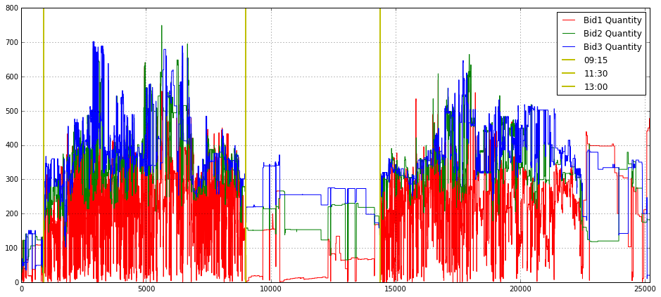
This block builds a single, annotated time-series plot of the top three bid‑side quantities so you can visually inspect intraday liquidity dynamics and identify regime changes relevant to execution and microstructure analysis. It starts by allocating a wide plotting canvas (16x7) and turning on a grid to make small fluctuations and relative levels easier to read; the three series — Bid1_Quantity_16_, Bid2_Quantity_16_, Bid3_Quantity_16_ — are then drawn on the same axes with distinct colors and labels so you can directly compare the immediate bid size at level 1, 2 and 3 over the session. Plot order matters for visibility when lines overlap, and labeling each series allows the legend to map colors back to queue depth.
The x-axis is explicitly constrained from 0 to 25,200, which in this context is being used as the trading session window (25,200 seconds = 7 hours). The hard limits focus the view on a single trading day and avoid distracting pre/post‑session noise. Three vertical lines (at x=900, 9000, 14,400) are drawn and annotated as 09:15, 11:30 and 13:00; these are anchors that segment the session into meaningful intraday periods (first 15 minutes, mid‑morning to lunch boundaries, and post‑lunch), which are commonly relevant for feature engineering, regime detection, or gating execution strategies because order flow and volatility often change at those times.
Why this matters for quant trading: visualizing the three top bid quantities together helps you spot liquidity depletion, sudden replenishment events, and persistent imbalances that would affect fill probability, market impact estimates, or smart‑order‑routing decisions. The vertical markers help correlate those microstructure events with canonical intraday phases that you may use as cut points for model training, evaluation windows, or different execution parameter sets.
import matplotlib.pyplot as plt
plt.figure(figsize = (16,9))
plt.subplot(221)
plt.grid()
plot(Bid1_Quantity_16_,label = ‘Bid1 Quantity’,color = ‘r’)
plot(Bid2_Quantity_16_,label = ‘Bid2 Quantity’,color = ‘g’)
plot(Bid3_Quantity_16_,label = ‘Bid3 Quantity’,color = ‘b’)
plt.xlim(0.0,25200)
plt.xlabel(”Second”)
plt.ylabel(”Quantity”)
#plt.axvline(x = 900 ,color = ‘y’,linestyle = ‘-’,label = ‘09:15’, linewidth = 2)
#plt.axvline(x = 9000 ,color = ‘y’,linestyle = ‘-’,label = ‘11:30’, linewidth = 2)
#plt.axvline(x = 14400 ,color = ‘y’,linestyle = ‘-’,label = ‘13:00’, linewidth = 2)
plt.legend(loc = 1,borderpad = 0.08,labelspacing = 0.08)

plt.subplot(222)
plt.grid()
plot(Ask1_Quantity_16_,label = ‘Ask1 Quantity’,color = ‘r’)
plot(Ask2_Quantity_16_,label = ‘Ask2 Quantity’,color = ‘g’)
plot(Ask3_Quantity_16_,label = ‘Ask3 Quantity’,color = ‘b’)
plt.xlabel(”Second”)
#plt.axvline(x = 900 ,color = ‘y’,linestyle = ‘-’,label = ‘09:15’, linewidth = 2)
#plt.axvline(x = 9000 ,color = ‘y’,linestyle = ‘-’,label = ‘11:30’, linewidth = 2)
#plt.axvline(x = 14400 ,color = ‘y’,linestyle = ‘-’,label = ‘13:00’, linewidth = 2)
plt.xlim(0.0,25200)
plt.legend(loc = 1,borderpad = 0.08,labelspacing = 0.08)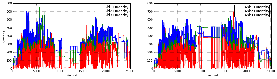
This block is constructing a two-panel visualization of order-book quantities over a trading day so you can inspect intra-day liquidity dynamics and spot imbalances or structural shifts. It opens a wide 16:9 canvas and allocates the top-left and top-right slots of a 2×2 grid for the bid and ask quantity series respectively; leaving the bottom row free implies the author intended to add more diagnostics (e.g., price, spread, or imbalance) below. The overall intent is exploratory — to make temporal patterns and sudden volume events in the top-of-book visible at second resolution.
In the first (top-left) panel the code plots the first three bid-level quantities (Bid1, Bid2, Bid3) as separate colored lines, turns on a grid for easier visual alignment, and labels axes with “Second” and “Quantity”. The x-axis is clipped to 0–25,200 seconds, which equals 7 hours: this ties the horizontal range to the full trading session so that each second index maps to a time-of-day. Plotting the top 3 bid levels lets you observe how available buying interest is stacked at the best prices and immediately behind them — useful for detecting liquidity suction or replenishment that matters for execution algorithms and short-term market-making strategies.
The second (top-right) panel mirrors the first but for the top three ask-level quantities (Ask1, Ask2, Ask3). Keeping bids and asks on separate subplots reduces visual clutter and makes asymmetries easier to read; if you want direct pointwise comparisons you could overlay them or compute a bid/ask imbalance series and plot that as a separate diagnostic. Both subplots use small legend padding and consistent coloring so you can quickly identify which depth-level is moving and whether changes are persistent or transient.
There are three commented vertical lines (axvline) at 900, 9,000 and 14,400 seconds that are left disabled — these are clearly intended to mark schedule landmarks like the opening micro-period and mid-session break points (for example, if your session starts at 09:00 then 900 s = 09:15, 9000 s ≈ 11:30, 14,400 s = 13:00). Turning those on helps correlate liquidity shifts with known market structure events (open/close auctions, lunch breaks, or known news windows). Finally, note that the plots do not fix y-limits or apply smoothing/normalization: that preserves raw quantity magnitudes which is good for execution sizing, but for comparative analyses you might want consistent y-scaling across panels, log-scaling to handle spikes, or a rolling-average overlay to reduce tick noise depending on the hypothesis you’re testing in your quant strategy.
plt.figure(figsize = (15,15))
plt.subplot(321)
plt.grid()
plot(Bid1_Quantity_16_,label = ‘Bid1 Quantity’,color = ‘r’)
plt.xlim(0.0,25200)
plt.axvline(x = 900 ,color = ‘y’,linestyle = ‘-’,label = ‘09:15’, linewidth = 2)
plt.axvline(x = 9000 ,color = ‘y’,linestyle = ‘-’,label = ‘11:30’, linewidth = 2)
plt.axvline(x = 14400 ,color = ‘y’,linestyle = ‘-’,label = ‘13:00’, linewidth = 2)
#plt.xlabel(”Second”)
plt.ylabel(”Quantity”)
plt.legend(loc = 1,borderpad = 0.08,labelspacing = 0.08)

plt.subplot(323)
plt.grid()
plot(Bid2_Quantity_16_,label = ‘Bid2 Quantity’,color = ‘g’)
plt.xlim(0.0,25200)
plt.axvline(x = 900 ,color = ‘y’,linestyle = ‘-’,label = ‘09:15’, linewidth = 2)
plt.axvline(x = 9000 ,color = ‘y’,linestyle = ‘-’,label = ‘11:30’, linewidth = 2)
plt.axvline(x = 14400 ,color = ‘y’,linestyle = ‘-’,label = ‘13:00’, linewidth = 2)
#plt.xlabel(”Second”)
plt.ylabel(”Quantity”)
plt.legend(loc = 1,borderpad = 0.08,labelspacing = 0.08)
plt.subplot(325)

plt.grid()
plot(Bid3_Quantity_16_,label = ‘Bid3 Quantity’,color = ‘b’)
plt.xlim(0.0,25200)
plt.axvline(x = 900 ,color = ‘y’,linestyle = ‘-’,label = ‘09:15’, linewidth = 2)
plt.axvline(x = 9000 ,color = ‘y’,linestyle = ‘-’,label = ‘11:30’, linewidth = 2)
plt.axvline(x = 14400 ,color = ‘y’,linestyle = ‘-’,label = ‘13:00’, linewidth = 2)
plt.xlabel(”Second”)
plt.ylabel(”Quantity”)
plt.legend(loc = 1,borderpad = 0.08,labelspacing = 0.08)
plt.subplot(322)

plt.grid()
plot(Ask1_Quantity_16_,label = ‘Ask1 Quantity’,color = ‘r’)
plt.xlim(0.0,25200)
plt.axvline(x = 900 ,color = ‘y’,linestyle = ‘-’,label = ‘09:15’, linewidth = 2)
plt.axvline(x = 9000 ,color = ‘y’,linestyle = ‘-’,label = ‘11:30’, linewidth = 2)
plt.axvline(x = 14400 ,color = ‘y’,linestyle = ‘-’,label = ‘13:00’, linewidth = 2)
#plt.xlabel(”Second”)
plt.ylabel(”Quantity”)
plt.legend(loc = 1,borderpad = 0.08,labelspacing = 0.08)

plt.subplot(324)
plt.grid()
plot(Ask2_Quantity_16_,label = ‘Ask2 Quantity’,color = ‘g’)
plt.xlim(0.0,25200)
plt.axvline(x = 900 ,color = ‘y’,linestyle = ‘-’,label = ‘09:15’, linewidth = 2)
plt.axvline(x = 9000 ,color = ‘y’,linestyle = ‘-’,label = ‘11:30’, linewidth = 2)
plt.axvline(x = 14400 ,color = ‘y’,linestyle = ‘-’,label = ‘13:00’, linewidth = 2)
#plt.xlabel(”Second”)
plt.ylabel(”Quantity”)
plt.legend(loc = 1,borderpad = 0.08,labelspacing = 0.08)

plt.subplot(326)
plt.grid()
plot(Ask3_Quantity_16_,label = ‘Ask3 Quantity’,color = ‘b’)
plt.xlim(0.0,25200)
plt.axvline(x = 900 ,color = ‘y’,linestyle = ‘-’,label = ‘09:15’, linewidth = 2)
plt.axvline(x = 9000 ,color = ‘y’,linestyle = ‘-’,label = ‘11:30’, linewidth = 2)
plt.axvline(x = 14400 ,color = ‘y’,linestyle = ‘-’,label = ‘13:00’, linewidth = 2)
plt.xlabel(”Second”)
plt.ylabel(”Quantity”)
plt.legend(loc = 1,borderpad = 0.08,labelspacing = 0.08)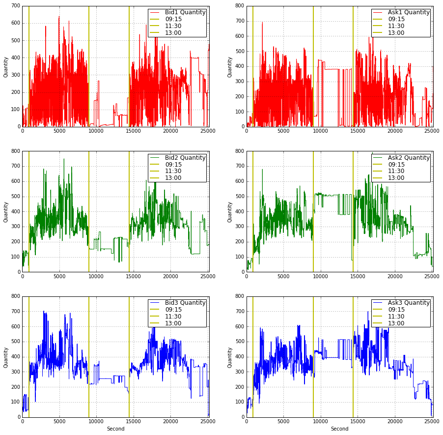
This code builds a 3×2 visualization of order‑book quantities so you can inspect intraday depth dynamics at the first three bid and ask levels. It starts by creating a large square canvas (figsize = 15×15) to give each small subplot enough room; the layout uses explicit subplot indices so the left column (321, 323, 325) is reserved for Bid1–Bid3 and the right column (322, 324, 326) for Ask1–Ask3. That arrangement intentionally separates side (bid vs ask) and level (1–3), which reduces overplotting and makes it easy to compare how liquidity evolves across price levels and across sides.
Each subplot draws a single time series of quantities (e.g., Bid1_Quantity_16_) with a consistent color scheme (red/green/blue for levels 1/2/3) and turns on a grid to make short‑term structure easier to read. The x axis is clipped to 0…25200 seconds; this enforces a common time window for all panels (the full trading interval of interest) so events line up vertically between plots. The clipping also prevents extreme timestamps or gaps from stretching the axis and hiding intraday patterns.
Every panel adds three vertical reference lines via axvline at x = 900, 9000, and 14400 and labels them as ‘09:15’, ‘11:30’, and ‘13:00’. These are deliberate intraday anchors — likely mapping seconds since market open to meaningful clock times — and they make it straightforward to correlate liquidity changes (spikes, thinning, or regime shifts) with known session boundaries or scheduled events. Placing identical markers on every subplot ensures you can visually compare how each depth level responds at the same moments.
The code also pays attention to readability: only the bottom row includes an x‑axis label (“Second”) to avoid cluttering every panel, while every subplot uses a y label “Quantity” so vertical scale meaning is explicit. Legends are positioned consistently at loc=1 (upper right) with small paddings to keep them out of the main data area but still informative; consistent labeling across panels lets you quickly identify the series and its color without scanning for a caption.
From a quant‑trading perspective this visualization is serving two main goals: diagnosing microstructure behavior (e.g., where liquidity concentrates, when depth collapses, asymmetric reactions between bid and ask) and generating features or hypotheses for models (e.g., intraday seasonality, level‑specific volatility, or event‑driven liquidity shifts). Practically, because the code repeats the same annotation and styling for each subplot, it would be straightforward to refactor into a small loop or helper to reduce duplication and to generalize the time markers if you need different session breakpoints or a different sampling frequency.
Bid1_Quantity_16_ = []
for i in range(0,25200,1):
    index = np.where(array(timestamp_time_second) <= i)[0][-1]
    Bid1_Quantity_16_.append(Bid1_Quantity_16[index])
At a high level this loop is taking an irregular, tick-level time series of the best bid quantity (Bid1_Quantity_16) and producing a fixed-length, per-second sequence for a 7‑hour window (25200 seconds). The outer loop walks second-by-second from 0 up to 25199; for each second i it looks up the most recent tick whose timestamp is at or before that second and copies that tick’s bid quantity into the output list. In other words, you are resampling the tick stream to a uniform one-second cadence using a “last known value” or forward‑fill rule so that the quoted bid quantity persists until the next tick updates it.
Mechanically, the code finds the index by selecting all indices where timestamp_time_second <= i and then taking the last of those indices ([0][-1]), and then it appends Bid1_Quantity_16 at that index into Bid1_Quantity_16_. The decision to use the last index <= i is deliberate: for market microstructure and backtesting we usually want the most recent known state at each evaluation timestamp (we do not extrapolate or interpolate between ticks because quotes are stepwise and you typically want right-continuous values). Using <= also means that if there is a tick exactly at second i, that tick is used; otherwise the previous tick is carried forward.
A few important caveats and reasons to revisit the implementation for production use in a quant setting. First, if there are seconds before the first tick (no timestamp <= i), the np.where (…) [0][-1] pattern will raise an IndexError — you need an explicit boundary check or an initial fill value to avoid crashes. Second, this loop repeatedly calls the search operation for every second which is O(T * N) in the worst case and will be slow for long windows or large tick arrays. If the timestamp array is sorted (which it should be), a much faster and clearer approach is to use np.searchsorted once (vectorized) or pandas’ reindex/resample with forward-fill; these give the same right-continuous semantics at far better performance. Finally, make sure timestamp_time_second is aligned to the same origin as i (e.g., seconds since session open), and that types and monotonicity are guaranteed; otherwise alignment errors will silently produce incorrect series.
import matplotlib.pyplot as plt
plt.figure(figsize = (16,7))
plt.grid()
plot(Bid1_Quantity_16_,label = ‘Bid1 Quantity’)
plt.xlabel(”Second”)
plt.ylabel(”Quantity”)
plt.axvline(x = 900 ,color = ‘y’,linestyle = ‘-’,label = ‘09:15’, linewidth = 2)
plt.axvline(x = 9000 ,color = ‘y’,linestyle = ‘-’,label = ‘11:30’, linewidth = 2)
plt.axvline(x = 14400 ,color = ‘y’,linestyle = ‘-’,label = ‘13:00’, linewidth = 2)
plt.xlim(0.0,25200)
plt.legend(loc = 1)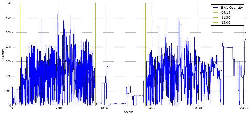
This block builds a simple time-series visualization of the best-bid quantity (Bid1_Quantity_16_) across a trading day so you can visually relate liquidity dynamics to fixed calendar times. It treats the series as an array indexed by elapsed seconds from a day-start (the x-axis label is “Second”), so the call to plot uses the series’ positional index as the time axis. The figure size and grid are set up first to make the chart legible and to help the eye follow level changes and short-lived spikes — useful when scanning for transient liquidity events or algorithmic activity.
Three vertical reference lines are drawn at x = 900, 9000 and 14400, labeled 09:15, 11:30 and 13:00 respectively. These numbers are in seconds: 900s = 15 minutes, 9000s = 2.5 hours, 14400s = 4 hours, so the code assumes the day starts at 09:00 (or otherwise that those second offsets correspond to the named clock times). Placing these markers directly on the chart lets you quickly correlate changes in Bid1 quantity with specific market schedule points (for example auction windows, known micro-structure shifts, or a lunch/auction break), which is crucial for understanding intraday liquidity patterns and for engineering time-dependent features in quant models.
The x-axis is clipped to the window 0.0–25200 seconds (7 hours), which enforces a consistent trading-hours view even if the underlying data contain extra timestamps or gaps; this keeps comparisons across days or instruments aligned. The legend and labels identify the series and the annotated times so the plot is immediately interpretable when reviewing many days or when presenting to stakeholders. In practice, this code implicitly assumes the data are sampled or reindexed to per-second resolution and aligned to the day-start — if that assumption doesn’t hold you’ll get misleading alignment between the plotted index and the labeled vertical lines. For robustness in a quant workflow you often want to explicitly convert timestamps to elapsed seconds, forward-fill or mark gaps, and consider smoothing or aggregating noisy per-second ticks before plotting so the visual highlights true liquidity structure rather than measurement noise.
import matplotlib.pyplot as plt
plt.figure(figsize = (16,7))
plt.grid()
plot(Bid2_Quantity_16_,label = ‘Bid2 Quantity’)
plt.xlim(0.0,25200)
plt.legend(loc = 1)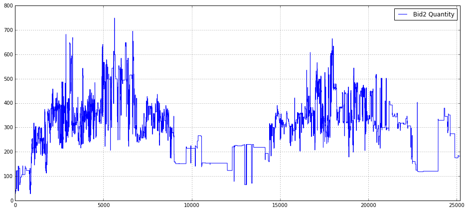
This snippet builds a focused time‑series visualization of a single order‑book quantity series so you can inspect liquidity at the second bid level over a trading session. First, it creates a wide plotting canvas (16×7 inches) so long horizontal time series are displayed with enough horizontal resolution to reveal intra‑session structure; the explicit figure size is chosen to make patterns and short‑lived events visible when you share or analyze a full‑day view. Enabling the grid provides regular visual reference lines, which helps when eyeballing level changes, jumps, or cyclic patterns in quantity.
The core drawing call plots the array/series Bid2_Quantity_16_ and attaches the label “Bid2 Quantity”. Depending on the object type, matplotlib will use either the Series’ datetime index (if it’s a pandas Series) or a numeric index (if it’s a numpy array); the plotted values represent the volume (or order count) at the second best bid level over time, which you inspect to detect liquidity shifts, microstructure events, or features useful for execution and alpha modeling. After plotting, the x‑axis is explicitly bounded to [0.0, 25200]; that constraint fixes the visible time window (likely representing a fixed session length or a fixed number of seconds/ticks), which prevents autoscaling to outliers and ensures consistency when comparing multiple plots or backtests. Using a hard limit like 25200 enforces a common frame of reference across figures, but it’s worth documenting or computing that limit from session metadata rather than leaving it as a “magic number.”
Finally, the legend is placed at location 1 (upper right) so the plotted series is identified on the figure; this is important whenever you overlay multiple series or want quick clarity on what each line means. In the context of quant trading, this plot is a quick diagnostic: it helps you validate feature behavior, spot anomalous order‑book activity, and decide whether further preprocessing (resampling, smoothing, outlier clipping, or alignment to timestamps) is needed before feeding the series into models or execution logic. Note that for production‑grade inspection you should add explicit axis labels and a title and prefer semantic legend/location strings (e.g., ‘upper right’) and timestamped x‑ticks if the index represents real times.
Bid3_Quantity_16_ = []
for i in range(0,25200,1):
    index = np.where(array(timestamp_time_second) <= i)[0][-1]
    Bid3_Quantity_16_.append(Bid3_Quantity_16[index])
This snippet is taking an irregular, tick-level sequence of bid sizes (Bid3_Quantity_16) and producing a regular, one-second resolved series of the same length (25200 seconds, i.e., 7 hours). The outer loop iterates over each second i in the target sampling grid. For each second it finds the last index in timestamp_time_second whose timestamp is <= i (the np.where(…)[0][-1] expression) and appends the corresponding bid size to the output list. In short, for every integer second it carries forward the most recent observed bid quantity — a last-observation-carried-forward (LOCF) resampling that produces a stepwise, time-aligned series.
import matplotlib.pyplot as plt
plt.figure(figsize = (16,7))
plt.grid()
plot(Bid3_Quantity_16_,label = ‘Bid3 Quantity’)
plt.xlim(0.0,25200)
plt.legend(loc = 1)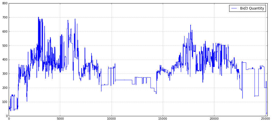
This block constructs a simple, focused visualization of the Bid3 quantity time series so you can inspect liquidity behavior at the third-best bid level over a trading interval. First it creates a wide figure (16x7 inches) to give horizontal space for high-frequency or long-duration time series — this reduces overplotting and makes short-lived spikes or microstructure patterns easier to see. Enabling the grid improves visual alignment so you can judge magnitudes and timing of moves at a glance, which is important when comparing small changes in order size across many observations.
The core action is plotting the array Bid3_Quantity_16_. That variable represents the quantity available at the third bid level (likely sampled at a regular interval), and plotting it directly surfaces liquidity dynamics such as step changes when orders are placed/cancelled, predictable intra-day patterns, or outliers that could indicate fat-finger events or data issues. The label provided on the series allows the legend to identify this trace when multiple series are overlaid.
Setting x-axis limits to (0.0, 25200) intentionally crops the view to the initial window of interest — 25200 is the number of seconds in 7 hours — so this is probably meant to focus the chart on a single trading session or a fixed analysis window rather than the entire dataset. That helps avoid displaying irrelevant pre/post-market data or very long histories that would compress the structure of a single session and hide microstructure effects. Finally, placing the legend at location 1 (upper-right) ensures the label is visible without covering the main body of the series in typical layouts; if you later add more series or annotations you may need to reposition or use an automated placement to avoid overlap.
Ask1_Quantity_16_ = []
for i in range(0,25200,1):
    index = np.where(array(timestamp_time_second) <= i)[0][-1]
    Ask1_Quantity_16_.append(Ask1_Quantity_16[index])
This loop is taking irregular, tick-level order-book updates and turning them into a fixed, one-second cadence series for the top-of-book ask quantity (Ask1). Conceptually you start with two parallel arrays: a timestamp array in seconds (timestamp_time_second) and an Ask1 quantity array sampled at those timestamps (Ask1_Quantity_16). The goal is to produce Ask1_Quantity_16_ — a length-25200 time series where each element is the most recent Ask1 value as of that whole-second timestamp.
Step by step: for each second i from 0 up to 25,199 the code finds the last index in the timestamp array whose timestamp is <= i, and then uses that index to read the corresponding Ask1 quantity and append it to the per-second output. Because the code uses the last index <= i, if there were multiple tick updates within the same second it picks the most recent one in that second; if there were no updates exactly at i it carries forward the last known value (last-observation-carried-forward). That design is intentional for quant workflows: many downstream features and risk calculations require regularly sampled inputs (returns, realized variance, microstructure features), so you need to align irregular updates onto a uniform grid.
A few important behavioral and robustness points to keep in mind. First, this is a forward-fill strategy: long gaps between ticks will produce repeated stale values for many consecutive seconds, which is appropriate when you want a snapshot series but can distort measures that assume frequent updates. Second, the current code relies on there being at least one timestamp <= i for every i; if the timestamp series starts after 0 the np.where(…)[0][-1] lookup will error. You should explicitly handle initial-empty-periods (for example, by pre-filling with NaN or the first observation). Third, the implementation is inefficient: calling np.where inside a Python loop is O(T*N) in practice and will be slow for large timestamp arrays and long time horizons. A much faster, more robust approach is to use a vectorized search on a sorted timestamp array (e.g., a searchsorted-style lookup for all integer seconds followed by a single index-based selection) or simply use a time-indexed Series/DataFrame and reindex with forward-fill. Finally, beware of variable-name confusion: Ask1_Quantity_16_ is the new list, while Ask1_Quantity_16 (without the trailing underscore) must be the original source array — ensure you don’t accidentally overwrite the source before this loop.
In short: the code produces a per-second snapshot series by carrying the last known ask quantity forward to every whole second, which is a common preprocessing step in quant trading to synchronize irregular order-book data onto a regular time grid. Make the edge-case handling explicit and switch to a vectorized method for scalability.
Ask2_Quantity_16_ = []
for i in range(0,25200,1):
    index = np.where(array(timestamp_time_second) <= i)[0][-1]
    Ask2_Quantity_16_.append(Ask2_Quantity_16[index])
This code is building a second-by-second version of an order-book quantity series so downstream quant models or backtests can consume a uniformly sampled feature. Conceptually, the original data consists of two parallel arrays: timestamp_time_second (irregular or event-driven times in whole seconds) and Ask2_Quantity_16 (the quantity observed at those event times). The loop walks through every second from 0 up to 25,199 and, for each second i, finds the most recent event whose timestamp is less than or equal to i, then copies that event’s Ask2_Quantity_16 into the per-second output array Ask2_Quantity_16_. The effect is “last observation carried forward” (LOCF): you hold the most recently observed quantity constant until an update arrives.
How the logic flows: for each i the code uses np.where(array(timestamp_time_second) <= i)[0][-1] to locate the index of the last timestamp that does not exceed i. That index is then used to pick the corresponding Ask2_Quantity_16 value and append it to the output list. Choosing the last matching index (the [-1]) enforces the forward-fill semantics and the <= ensures that an event occurring exactly at second i is used for that second’s value.
Why this is done in quant trading: many models and backtests require fixed-frequency inputs (per-second, per-minute, etc.) even though market messages arrive asynchronously. By converting irregular event data into a regular time grid and using LOCF, you preserve the most recent market state at every evaluation time — which is usually the correct semantic for features like displayed quantity that persist until changed. That alignment is critical for feature engineering, aggregation, and ensuring model inputs and target computations are synchronized.
Important assumptions and pitfalls to watch for: the code assumes timestamp_time_second is sorted ascending and that there is at least one timestamp <= i for every i in the loop; otherwise np.where(…)[0][-1] will raise an IndexError (this often occurs if the first timestamp is greater than 0). It also assumes timestamps are integer seconds and that Ask2_Quantity_16 is indexed the same way as timestamp_time_second. Performance is another concern: this is O(T * log? or O(T * N) depending on np.where internals) because each second performs a search over the timestamps; for long time ranges or large event counts this will be slow.
Ask3_Quantity_16_ = []
for i in range(0,25200,1):
    index = np.where(array(timestamp_time_second) <= i)[0][-1]
    Ask3_Quantity_16_.append(Ask3_Quantity_16[index])
This loop is building a regular, per-second time series of the level-3 ask quantity by mapping each integer second to the most recent observed market value at or before that second. Concretely, for every second i from 0 up to 25,199 the code finds the last index in the timestamp_time_second array whose value is <= i, then appends the Ask3_Quantity_16 value at that index to the output list. In other words, it implements a last-observation-carried-forward (forward-fill / “as-of”) resampling: every second gets assigned the latest known Ask3 quantity available up to that time.
Why this is done: many quant workflows and backtests require features sampled on a fixed time grid (per-second here) so that models, metrics, or simulators see regularly spaced inputs. Orderbook updates arrive irregularly; mapping them onto a uniform timeline with the most recent observation preserves the intraday state without inventing values between updates. Using the condition <= i ensures we pick the latest observation at or before each second, which is appropriate when you want market state “as of” that second.
Important assumptions and edge cases to be aware of: this presumes timestamp_time_second is monotonic (sorted). If it is not sorted, the “last index where <= i” does not reliably represent chronological last observation and will produce incorrect mapping. If there are seconds before the first recorded timestamp, np.where(…)[0][-1] will raise an IndexError — you should decide whether to fill those leading seconds with NaN, zeros, or a defined default. Also, if many updates occur inside the same second, the code picks the last one within that second, which is usually the desired behavior for an “as-of” view.
Performance and robustness concerns: the code calls np.where on a (re)constructed array(timestamp_time_second) every iteration, so it repeats the same scan thousands of times. That makes the routine O(T * N) in the worst case (T = 25,200 seconds, N = number of timestamps) and will be slow for typical tick-level volumes. It also continuously converts timestamp_time_second to an array if that conversion happens inside the loop. A more robust approach is to use a vectorized search (np.searchsorted on a precomputed numpy array) or to use pandas’ reindex/resample with asof/ffill functionality, both of which are O(N + T) and handle edge cases more cleanly. Finally, consider making the target time range dynamic (based on trading hours or data span) and explicitly handling leading missing values and any timezone/epoch alignment issues so downstream models and backtests see consistent, well-defined inputs.
import matplotlib.pyplot as plt
plt.figure(figsize = (16,7))
plt.grid()
plot(Ask1_Quantity_16_,label = ‘Ask1 Quantity’)
plt.xlim(0.0,25200)
plt.legend(loc = 1)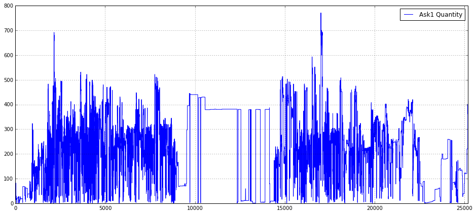
This block creates a wide, readable time-series plot of the top-of-book ask volume for the instrument labeled “16” so you can visually inspect liquidity dynamics. The code first allocates a rectangular canvas (16×7 inches) and turns on a grid to give you horizontal/vertical reference lines, which makes it easier to judge the magnitude and timing of changes in the series. It then draws the series Ask1_Quantity_16_ as a single line and tags it with the label “Ask1 Quantity” so the plotted trace is self-describing in the legend.
From a data-flow perspective, matplotlib uses the series index as the x-axis by default, so the visualization shows Ask1 quantities over whatever implicit time or sample index your array carries. The explicit x-axis limit xlim(0.0, 25200) zooms the view to the integer range 0 → 25,200, which is deliberate: 25,200 seconds equals seven hours, so this constrains the plot to a single trading-session window (or any intended 7-hour slice) and ensures consistent alignment when you compare multiple sessions or instruments.
Finally, placing the legend at location 1 (upper-right) is a simple, pragmatic choice to keep the annotation out of the main plot area in most cases and to future-proof the code when you add more series. The net business purpose is to enable quick visual detection of liquidity events — spikes, dry-ups, or regime shifts at the best ask — which are critical signals for execution algorithms, market-impact estimation, and feature engineering in quant strategies. If you plan to do repeated visual QA, consider ensuring the x-axis truly represents the intended time base (seconds vs. datetimes) and, for high-frequency noisy traces, think about downsampling or smoothing to reveal mid- to larger-scale patterns.
import matplotlib.pyplot as plt
plt.figure(figsize = (16,7))
plt.grid()
plot(Ask2_Quantity_16_,label = ‘Ask2 Quantity’)
plt.xlim(0.0,25200)
plt.legend(loc = 1)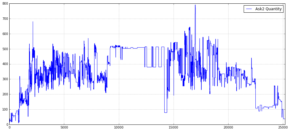
This small block is a focused visualization step whose goal is to make the time evolution of the second-level ask-side quantity for a particular instrument (Ask2_Quantity_16_) immediately interpretable for a quant workflow. First, we create a wide, single-panel figure (16x7) so the intraday structure is visible with enough horizontal resolution to display many time steps; choosing a large aspect ratio is deliberate for time-series where patterns and transient spikes matter. Enabling the grid improves visual readibility of horizontal and vertical reference lines so you can quickly judge magnitudes and timing of liquidity events.
The central action is plotting Ask2_Quantity_16_ as a labeled series; the label ensures the plotted line can be identified when multiple series are shown or when saving figures for later review. The explicit x-axis limit of (0.0, 25200) constrains the view to a fixed intraday window — in practice this maps the array index to a trading-day span (25200 is likely an integer number of seconds or ticks chosen to correspond with the period of interest). Limiting the x-range focuses analysis on the main session, removes far-out indices or tails that would compress the main structure, and makes it easier to compare this plot across days or instruments on a consistent time grid.
Finally, the legend placed in the upper-right (loc=1) keeps the label unobtrusive while remaining visible, and the overall arrangement is intended to serve two operational purposes in quant trading: quick human validation of the raw order-book quantity series (spotting data quality issues, gaps, or timestamp misalignment) and exploratory detection of microstructure phenomena — e.g., liquidity depletion, periodicity, or spikes around known events — that can inform feature engineering, intraday regime classification, or trigger rules for execution algorithms.
import matplotlib.pyplot as plt
plt.figure(figsize = (16,7))
plt.grid()
plot(Ask3_Quantity_16_,label = ‘Ask3 Quantity’)
plt.xlim(0.0,25200)
plt.legend(loc = 1)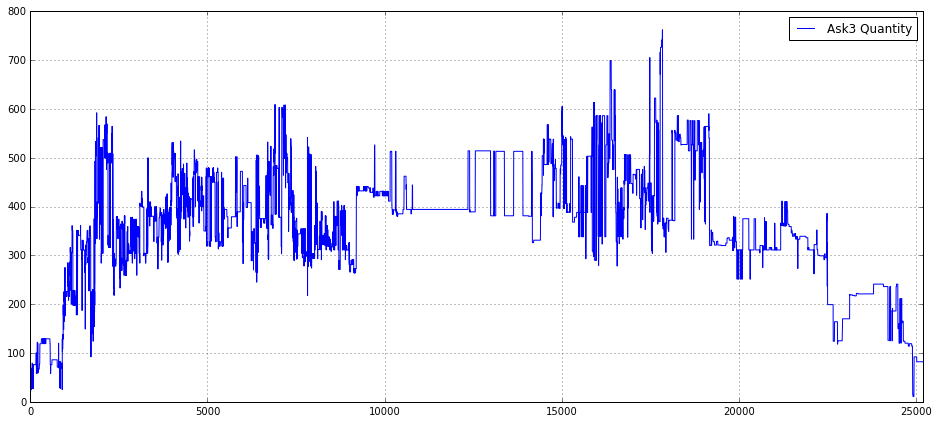
This block is setting up a visual inspection of a single time series — the Ask3_Quantity_16_ — with the intention of making patterns in that order-book variable visible across a full trading session. The code first creates a wide plotting canvas (16x7) so that time-dependent structure and transient spikes are not compressed; for quant trading work you often need horizontal space to see intraday seasonality, clusters of liquidity events, and the fine structure of order-flow spikes that could become features. Turning on the grid is a deliberate readability choice: horizontal and vertical gridlines make it easier to estimate magnitudes and align events in time when you’re eyeballing relationships between order-book quantities and price moves.
Next, the series itself is rendered with a label of ‘Ask3 Quantity’, so it will appear in the legend and be identifiable when multiple series are overlaid. Plotting the Ask3 quantity (level-3 ask size) is a common diagnostic for liquidity dynamics — you’re looking for changes in resting size that precede price moves, consolidations, or episodes of liquidity withdrawal. The hard x-axis limit of 0.0 to 25200 is meaningful: it forces a consistent timescale across charts (25200 seconds = 7 hours), which is useful when you want to compare multiple days or multiple instruments on the same horizontal span. That consistency helps detect intraday patterns and align events across runs, but it also has two trade-offs: it will clip data outside that window and will show empty space if the series is shorter than 25200 indices, so you should ensure your index-to-time mapping matches this scale.
Finally, the legend is placed in location 1 (upper-right) so the plotted label is visible without overlapping typical mid-chart activity. In summary, this snippet is about turning raw Ask3 quantity data into a consistently-scaled, readable diagnostic plot to support feature discovery and event inspection in a quant trading workflow; be mindful that using integer x-limits and not converting indices to human-friendly timestamps can obscure interpretation, so consider aligning the x-axis with actual timestamps or annotating known market events when you move from exploration to production diagnostics.
hist(array(bas_16_one_second)/5.0,bins = 50)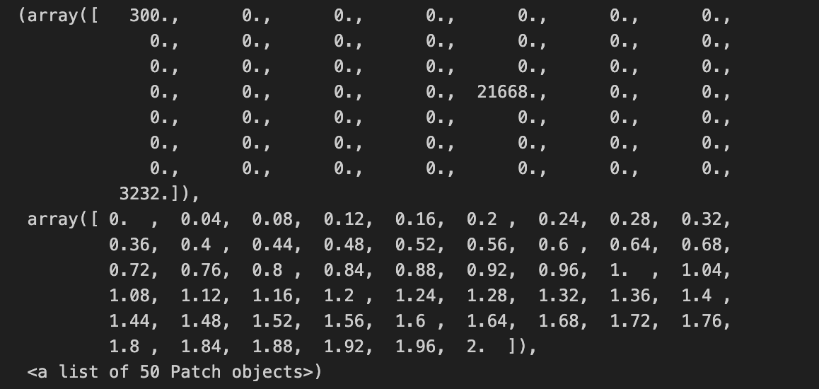
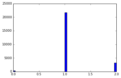
This line takes your raw per-second series (bas_16_one_second), ensures it’s treated as a numeric array, rescales every element by dividing by 5.0, and then builds a 50-bin histogram to visualize the empirical distribution. Converting to an array first guarantees we get elementwise arithmetic (so the division produces a vector of scaled values rather than a single scalar or object-level operation), which is important if bas_16_one_second can be a list-like or other iterable. The division by 5.0 is a deliberate rescaling step — in quant trading this is usually done to convert the raw metric into a consistent unit (for example, from ticks to price change per 5 seconds, from total volume to volume per standard lot, or to normalize amplitudes so different instruments are comparable). Doing the scaling up front keeps the histogram’s bins interpretable in that target unit rather than the original raw measurement.
Choosing bins=50 is a pragmatic trade-off between resolution and noise: with 50 bins you get reasonably fine-grained detail on the distribution shape (peaks, shoulders, and tail behavior) without making each bin so narrow that sampling noise dominates. From a quant perspective the resulting histogram is used to inspect distributional properties relevant for modeling and risk — spotting heavy tails, skew, clustering or outliers that might invalidate Gaussian assumptions, influence volatility estimates, or require robust preprocessing.
min_Ask1_16_time_series = []
min_Ask1_16_time_series.append(0)
for i in range(1,len(Ask1_16),1):
    min_Ask1_16_time_series.append(min(Ask1_16[i:]))
This small block is building a time series of suffix minima from an Ask price sequence (Ask1_16) — in other words, for each time index it records the minimum ask price observed from that index forward. The code starts by creating an output list and appending a 0 as the first element; then it iterates i from 1 to the last index and appends min(Ask1_16[i:]) for each i. Concretely, the element at position i in min_Ask1_16_time_series (for i >= 1) is the minimum of Ask1_16 over indices [i, i+1, …, end]. The explicit 0 at position 0 is a placeholder so the output list ends up the same length as Ask1_16 — the author has chosen not to compute a suffix minimum for index 0 (or to represent it with a sentinel).
Why you would compute this in a quant context: suffix minima give you the best (lowest) ask price you could have achieved by waiting from each observation forward, which is useful for labeling supervised problems (e.g., “how low will the ask go in the future?”), estimating potential slippage or execution opportunity, or constructing event-based targets for backtests. Whether the minimum should include the current price matters for the interpretation: the current code includes Ask1_16[i] in the minimum (because it takes Ask1_16[i:]), so the suffix minimum can be equal to the current price — if you want to measure future improvement strictly after the current tick, you should use Ask1_16[i+1:].
max_Bid1_16_time_series = []
max_Bid1_16_time_series.append(0)
for i in range(1,len(Bid1_16),1):
    max_Bid1_16_time_series.append(max(Bid1_16[i:]))
This snippet is building a forward-looking “peak” series from an existing Bid1_16 price series: for each time index i it records the maximum bid seen from i (inclusive) to the end of the array, and it prepends a single zero to keep the output the same length as the input. Stepping through the flow: the list is created and seeded with 0 as the zeroth element; the loop starts at index 1 and for each i computes max(Bid1_16[i:]) — that is, the highest bid that occurs at or after time i — and appends that value. By the loop’s final iteration (i == len(Bid1_16) — 1) it appends the last element of Bid1_16, so the resulting list has one entry per original timestamp.
Why you would do this in quant trading is straightforward: you often need a label or feature that captures the best possible future price movement from a given entry point (for example to estimate potential profit, the peak reachable after entry, or to determine whether a price will ever exceed a threshold after a given time). This code produces that “future-peak” signal for each time point (except the zeroth index, which this code currently represents with a zero placeholder).
There are a couple of important behavioral and correctness details to be aware of. First, the choice to seed the series with 0 is a design decision that can materially affect downstream decisions or model training: zero may be an inappropriate placeholder if bids are strictly positive (it will artificially lower metrics) or if you expect NaN/missing to indicate absence of future information. Second, the loop uses max(Bid1_16[i:]) which includes the current index i in the future window; if your intent is to measure the maximum strictly after the current timestamp, you should shift the slice to i+1. Third, this implementation is O(n²) in time and allocates many intermediate slices, because each iteration computes a new max over an increasingly large suffix; for long tick series that will be slow and memory inefficient.
To address performance and robustness, compute the forward maximum in a single O(n) pass from right to left: maintain a running max, update it with each element as you traverse backwards, and store the running max values (then reverse if needed). That avoids repeated slicing and is linear time with constant extra memory overhead beyond the output. Also consider whether the initial placeholder should be NaN, the full-array max, or omitted, and be explicit about whether the window is inclusive or exclusive of the current timestamp — align that choice with how you will use this series in labeling, backtesting, or feature engineering so you do not leak future information or bias model targets.
import matplotlib.pyplot as plt
plt.figure(figsize = (16,7))
plt.grid()
plot(Ask1_16[0:len(Ask1_16)],label = ‘Ask1’,color = ‘b’)
#plot(Ask2[0:data_trade_time_series_0900_0930],label = ‘Ask2’)
#plot(Ask3[0:data_trade_time_series_0900_0930],label = ‘Ask3’)
plot(min_Ask1_16_time_series[0:len(Ask1_16)],label = ‘min Ask1 (close)’, linewidth = 2,color = ‘y’)
plot(max_Bid1_16_time_series[0:len(Ask1_16)],label = ‘max Bid1 (close)’, linewidth = 2,color = ‘g’)

plot(Bid1_16[0:len(Ask1_16)],label = ‘Bid1’,color = ‘r’)
#plot(Bid2[0:data_trade_time_series_0900_0930],label = ‘Bid2’)
#plot(Bid3[0:data_trade_time_series_0900_0930],label = ‘Bid3’)
plt.ylim(6710,6810)
plt.legend(loc = 4)
index1 = np.where(np.array(max_Bid1_16_time_series[0:len(Ask1_16)]) == max(max_Bid1_16_time_series[0:len(Ask1_16)]))[0][-1]
plt.axvline(x = index1 ,color = ‘g’,linestyle = ‘-’,label = 0.4, linewidth = 2)
index2 = np.where(np.array(min_Ask1_16_time_series[0:len(Ask1_16)]) == unique(min_Ask1_16_time_series[0:len(Ask1_16)][1]))[0][-1]
plt.axvline(x = index2 ,color = ‘y’,linestyle = ‘-’,label = 0.4, linewidth = 2)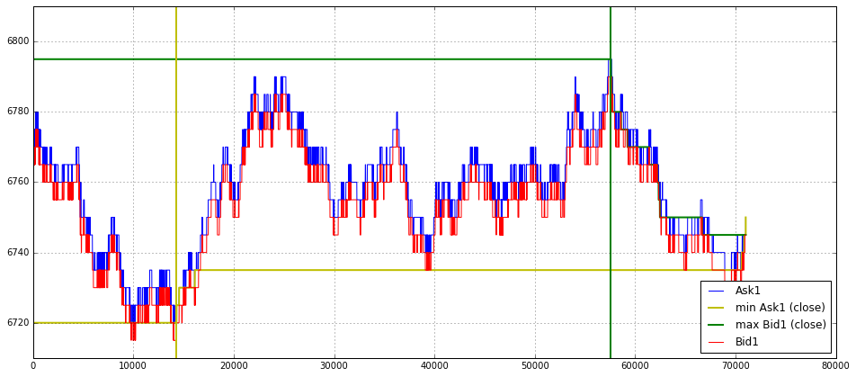
This block is a small visualization routine whose practical purpose is to inspect top-of-book price evolution and highlight two extreme events in that series so you can reason about liquidity / entry points in the trading session.
First, the code sets up a wide figure and enables a grid so the plotted price traces are easy to read. Every plotted series is explicitly sliced with [0:len(Ask1_16)] to force the same length for each trace; that’s a defensive move to avoid mismatched-length errors or unintended broadcasting when the underlying arrays may have different lengths. In a quant-trading context we want all series aligned on the same index (time buckets, ticks, or intervals) so price relationships (bid vs ask, min/max) are visually comparable.
Next, the routine draws four overlaid series: Ask1_16 in blue and Bid1_16 in red are the live top-of-book ask and bid traces (the most important market-facing prices). Two thicker, colored series are overplotted to emphasize envelope information: min_Ask1_16_time_series (yellow) and max_Bid1_16_time_series (green) — these appear to be precomputed per-interval minima or maxima (note the labels use “(close)”, which implies they might represent an extremum across a subwindow such as close-of-interval values). Visually emphasizing these max/min series helps you quickly see when the active top-of-book touches or breaks prior local extremes, which is useful for identifying breakout or mean-reversion opportunities.
The y-axis is clipped with plt.ylim(6710,6810) to focus the view on the price band of interest and reduce visual noise; limiting the vertical range makes spread changes and small penetrations easier to spot. A legend is placed in the lower-right (loc=4) to keep the chart readable.
After plotting, the code computes two indices to mark with vertical lines. index1 finds the last occurrence of the maximum value in max_Bid1_16_time_series: it converts that slice to an array, compares to the overall maximum, uses np.where to get indices, and picks [0][-1] to take the final occurrence. Plotting a vertical green line at index1 highlights the most recent time when the bid envelope reached its maximum — that’s meaningful because the most recent extreme can be a reference for resistance or a liquidity cluster that matters for trade execution decisions.
index2 attempts to do something analogous for the min_Ask1_16_time_series, but the expression as written is fragile and likely incorrect. The code uses unique(min_Ask1_16_time_series[0:len(Ask1_16)][1]) which effectively takes the element at position 1 of the slice and then wraps it in np.unique; the equality test therefore finds positions equal to that single element. If the intent was to find the index of the global minimum or the last occurrence of a particular extreme, this is the wrong approach. A clearer, more robust intent would be either:
- to locate the global minimum: idx = np.where(arr == np.min(arr))[0][-1], or simply idx = np.argmin(arr) if you want the first minimum, or
- to pick a specific unique value (for example the second unique value) you should call np.unique(arr)[1] explicitly, not np.unique(arr[1]).
Choosing [-1] (last occurrence) in both index computations is deliberate: when multiple equal extrema exist, the code picks the most recent one so the vertical marker points to the latest event, which is typically what you care about for live decision-making.
import time
start = time.time()
min15_Ask1_time_series = []
min15_Ask1_time_series.append(0)
i = 0
for j in range(1,len(Ask1_16),1):

    index = np.where(array(timestamp_time_second) <= i)[0][-1]
    #print ‘i = %d’%(i)
    #print ‘index = %d’%(index)
    #print ‘timestamp = %d’%(timestamp_time_second[index])
    if i < 25200 - 900:
            index_15_min = np.where(np.array(timestamp_time_second[index:]) >= i + 900)[0][0]
    min_15 = min(Ask1_16[(index+1):(index + 1 + index_15_min + 1)])
    min15_Ask1_time_series.append(min_15)
    if timestamp_time_second[j] > i:
        i = i + 1

#max_Bid1_time_series = []
#max_Bid1_time_series.append(0)
#for i in range(1,len(Ask1),1):
#    max_Bid1_time_series.append(max(Bid1[i:]))
end = time.time()
print “Total time = %f”%(end - start)
This block is building a time-series of 15-minute forward minima of the ask-side top-of-book (Ask1_16) aligned to a running second counter; in quant terms, you can think of it as producing a label or feature that answers “what was the lowest ask price in the next 15 minutes from this point in time?” for each observed snapshot. The outer loop iterates across the sequence of order-book snapshots (the loop variable j is only used to advance time), while the integer i acts as a current-second clock that the code uses to locate the most recent snapshot at or before that second and then to find the snapshot at/after i + 900 seconds (900 = 15 minutes). The result appended each iteration is the minimum Ask1 price observed between the snapshot immediately after the current-second index and the first snapshot at or after 15 minutes ahead.
Concretely, for each iteration the code first finds index = last position where timestamp_time_second <= i, i.e. the most recent snapshot that occurred at or before the current second i. Next it computes index_15_min by searching forward from that index for the first snapshot whose timestamp is >= i + 900. This gives an offset that identifies the end of the 15-minute forward window in terms of snapshot index rather than raw seconds. The code then slices Ask1_16 from the element after the current index up to that forward index and takes the minimum; that minimum is appended to min15_Ask1_time_series. This is how the code converts irregularly timed snapshots into a fixed 15-minute forward metric: it maps the current-second clock to snapshot indices, then computes the min across the snapshots that fall inside the next 15 minutes.
The loop advances the second-counter i in an event-driven way: if the timestamp at the current loop position j exceeds i, it increments i by one second. Because j steps through snapshots and i steps through integer seconds only when a new snapshot’s timestamp goes beyond the current second, the algorithm effectively walks time forward as snapshots arrive, aligning the forward-window calculations to second granularity while using the actual snapshot times to delimit the window boundaries.
import time
start = time.time()
max_Bid1_time_series = []
max_Bid1_time_series.append(0)
i = 0
for j in range(1,len(Bid1_16),1):

    index = np.where(array(timestamp_time_second) <= i)[0][-1]
    #print ‘i = %d’%(i)
    #print ‘index = %d’%(index)
    #print ‘timestamp = %d’%(timestamp_time_second[index])
    if i < 25200 - 900:
            index_15_max = np.where(np.array(timestamp_time_second[index:]) >= i + 900)[0][0]
    max_15 = max(Bid1_16[(index+1):(index + 1 + index_15_max + 1)])
    max_Bid1_time_series.append(max_15)
    if timestamp_time_second[j] > i:
        i = i + 1

end = time.time()
print “Total time = %f”%(end - start)
This loop’s high-level goal is to build a time series of “15-minute forward maximum” values for the best-bid (Bid1_16) so you can use a forward-looking label or feature for a quant-trading model (for example, to predict whether the best bid will reach a certain level within the next 15 minutes). The code walks through tick data (indexed by j) while maintaining an auxiliary second-counter i that maps the high-resolution tick timestamps to whole seconds. For each iteration it finds the most recent tick index at or before the current second i, locates the tick index that first reaches at least i + 900 seconds (i.e., 15 minutes later) and then computes the maximum Bid1_16 across that forward slice. That maximum is appended to max_Bid1_time_series. The run is timed to measure total wall-clock cost.
More concretely, the logic flow is:
- i starts at 0 and is intended to represent elapsed seconds from session start. timestamp_time_second is assumed to be a monotonic array of tick timestamps expressed in whole seconds.
- For each tick index j (looping from 1 to len(Bid1_16)-1) the code maps the current second i to the corresponding tick index using index = np.where(timestamp_time_second <= i)[0][-1]. This gives the last tick that occurred at or before second i.
- If we are at least 15 minutes before the session end (i < 25200–900; here 25200 sec looks like a session length constant), the code finds the offset index_15_max into timestamp_time_second[index:] of the first tick whose timestamp is >= i + 900 seconds. That offset plus the base index gives the tick at or just after the 15-minute horizon.
- Using that offset, it slices Bid1_16 from just after the current index up through the determined future index and computes max_15 = max(…) — the 15-minute forward maximum of the best bid — and appends it to max_Bid1_time_series.
- At the end of the loop body, the code increments i by one second only when timestamp_time_second[j] > i, which effectively steps the second-counter forward when the current tick moves past the current second. This makes i climb in one-second increments keyed to tick timestamps; multiple ticks that fall inside the same second will reuse the same i and therefore the same forward-max result.
- Outside the loop the code prints the elapsed processing time. The initial max_Bid1_time_series.append(0) is a placeholder to align indices (presumably so the returned list lines up with some other series), and the loop appends one value per iteration (so length and alignment considerations matter for downstream use).
Why this is done this way (the “why” behind key decisions):
- Mapping i (seconds) to a tick index lets you compute a forward-looking label based on a fixed time horizon (900 seconds) even though the original data are irregularly spaced ticks. Many trading strategies and supervised labels are defined on fixed time horizons rather than fixed tick counts, so this mapping is necessary.
- Using the first timestamp >= i + 900 ensures the forward window extends to at least the 15-minute boundary; using max over that window gives a conservative label for “how high the bid reached” in that horizon, which is useful for max-reward / breakout objectives.
- Incrementing i only when timestamp_time_second[j] > i causes the algorithm to produce repeated entries for ticks occurring in the same second (which may be intentional if you want one forward-max per tick but keyed by second) and to advance the second-counter in lockstep with ticks.
Important correctness and performance notes:
- Off-by-one and edge-case risk: the slice uses (index+1):(index + 1 + index_15_max + 1). Given how index_15_max is computed (as an offset into timestamp_time_second[index:]), the various +1s are confusing and easily produce an extra element or exclude the intended boundary. You should verify whether you want the window to include the tick at index (current tick), the tick at the 15-minute boundary, or only strictly between them, and simplify the slice accordingly.
- Session-end handling bug: index_15_max is only defined inside the if i < 25200–900 branch. When i is within the final 15 minutes (i >= 25200–900) the code will not set index_15_max but will still attempt to compute max_15 and append it — that will raise a NameError. If the intention is to stop generating forward labels in the final 15 minutes, add an explicit else branch (or break/continue) to avoid using an undefined variable.
- Efficiency: the code repeatedly calls np.where on the full timestamp array inside the loop, converts slices to arrays, and computes Python max on slices — this is O(N * M) work in the worst case and will be slow on large tick streams. Because timestamp_time_second is sorted, a far faster approach is to precompute mappings with np.searchsorted (vectorized), or to compute all “end” indices once (searchsorted(timestamp_time_second, timestamp_time_second + 900)) and then compute forward maxima in one pass. For sliding-window maxima, a deque-based rolling-max or a vectorized cumulative max on a reversed array (or numba/Cython) will be much faster and more memory-efficient.
- Repeated dtype conversions: the code does np.array(timestamp_time_second[index:]) inside the loop — avoid repeated conversions by ensuring timestamp_time_second is already a NumPy array and use slicing/searchsorted directly.
import matplotlib.pyplot as plt
plt.figure(figsize = (16,6))
plt.grid()
plot(Ask1_16[0:len(Ask1_16)],label = ‘Ask1’,color = ‘b’)
#plot(Ask2[0:len(Ask1)],label = ‘Ask2’)
#plot(Ask3[0:data_trade_time_series_1530_1600],label = ‘Ask3’)
plot(min15_Ask1_time_series[0:len(Ask1_16)],label = ‘min Ask1(15 min)’, linewidth = 1.2,color = ‘y’)
plot(max_Bid1_time_series[0:len(Ask1_16)],label = ‘max Bid1(15 min)’, linewidth = 1.2,color = ‘g’)

plot(Bid1_16[0:len(Bid1_16)],label = ‘Bid1’,color = ‘r’)
#plot(Bid2[0:len(Ask1)],label = ‘Bid2’)
#plot(Bid3[0:data_trade_time_series_1530_1600],label = ‘Bid3’)
plt.ylim(6710,6805)
plt.xlabel(”Microsecond”)
plt.ylabel(”A50 Price”)
plt.legend(loc = 1)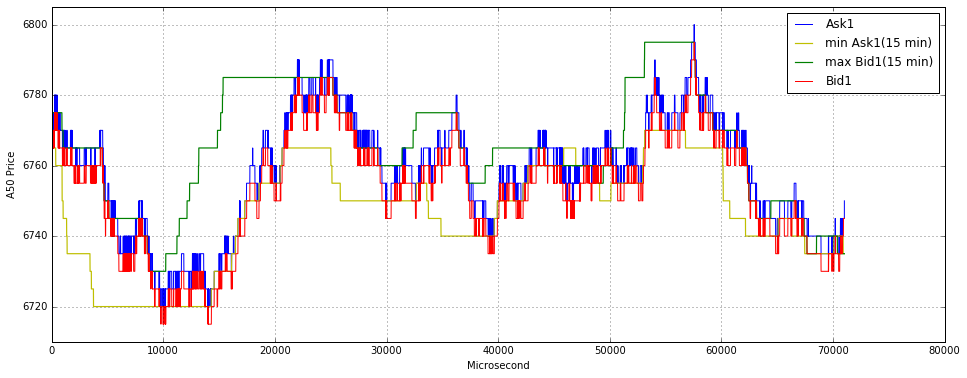
This block’s immediate goal is visual inspection: it overlays raw bid and ask microstructure with 15-minute aggregate extrema so you can quickly see how short-term extremes constrain or diverge from the live quote stream. We begin by creating a wide plotting canvas and enabling a grid to make small vertical deviations easy to see at a glance — useful when you’re evaluating microsecond-resolution moves in an instrument such as A50. The figure width is intentionally large to spread out dense tick data so patterns and clusters aren’t visually compressed.
Next, the live ask series Ask1_16 is drawn first as the primary reference line (blue). The code slices every series to the length of Ask1_16 before plotting; this is a pragmatic way to avoid shape-mismatch errors and to ensure all overlaid series share the same x-index range. Practically, that means the x-axis here is the integer index of ticks (the code labels it “Microsecond”), not a datetime axis — so the plot shows relative sequence order rather than absolute timestamps. If you need exact timing for latency or event alignment analysis, you’d replace these slices with a timestamp-aligned index.
After plotting the raw ask stream, the script overlays two 15-minute aggregated boundary series: min15_Ask1_time_series (yellow) and max_Bid1_time_series (green). These are drawn with slightly increased linewidth to visually separate the longer-window extrema from the noisy tick lines; the extrema act as contextual bands that indicate recent local support/resistance or liquidity ceilings/floors. Displaying the ask-side 15-min minima and the bid-side 15-min maxima together helps you evaluate spread behavior and whether the current quote is approaching or breaking out of the short-term range — a useful signal for entry/exit logic, stop placement, or detecting regime shifts.
The live bid stream Bid1_16 is plotted afterwards in red, so it sits on top of earlier layers and makes the current bid/ask spread immediately visible where the two primary tick lines converge or diverge. A couple of extra series (Ask2/Ask3, Bid2/Bid3) are commented out; that indicates the author considered plotting deeper levels but chose to focus on top-of-book dynamics for clarity. Plotting order matters: lines drawn later can occlude earlier ones, so the chosen order prioritizes visibility of the live bid and the aggregated extrema relative to the live ask.
Finally, the plot enforces a tight y-limits window (6710–6805) and labels the axes, which forces focus on the relevant price band and prevents autoscaling from flattening the fine structure you care about in quant work. The legend is placed in the upper-right to explain colors and styles. Collectively, this visualization gives you a fast diagnostic of microstructure: whether the book is tight or widening, whether price is trading near recent 15-minute extremes (possible breakout/mean-reversion signals), and whether stale or anomalous quotes appear — all information you’d use to validate models, tune execution algorithms, or trigger strategy rules.
import matplotlib.pyplot as plt
plt.figure(figsize = (16,6))
plt.grid()
plot(Ask1_16[0:len(Ask1_16)],label = ‘Ask1’,color = ‘b’)
#plot(Ask2[0:len(Ask1)],label = ‘Ask2’)
#plot(Ask3[0:data_trade_time_series_1530_1600],label = ‘Ask3’)
plot(min15_Ask1_time_series[0:len(Ask1_16)],label = ‘min Ask1(15 min)’, linewidth = 1.2,color = ‘y’)
plot(max_Bid1_time_series[0:len(Ask1_16)],label = ‘max Bid1(15 min)’, linewidth = 1.2,color = ‘g’)
plt.axvline(x = index11_16 ,color = ‘y’,linestyle = ‘-’,label = ‘11:30’, linewidth = 2)
plt.axvline(x = index13_16 ,color = ‘y’,linestyle = ‘-’,label = ‘13:00’, linewidth = 2)
plot(Bid1_16[0:len(Bid1_16)],label = ‘Bid1’,color = ‘r’)
#plot(Bid2[0:len(Ask1)],label = ‘Bid2’)
#plot(Bid3[0:data_trade_time_series_1530_1600],label = ‘Bid3’)
plt.ylim(6710,6805)
plt.legend(loc = 1)

plt.figure(figsize = (16,3))
plt.grid()
plot(rise_ratio_ask_16,label = ‘Ask1 Rise Ratio’, linewidth = 1.2,color = ‘b’)

plt.axhline(0.4,color = ‘g’,linestyle = ‘-’,label = 0.4, linewidth = 1.2)
plt.axhline(0.15,color = ‘r’,linestyle = ‘-’,label = 0.15, linewidth = 1.2)
plt.axhline(-0.15,color = ‘g’,linestyle = ‘-’,label = -0.15, linewidth = 1.2)
plt.axhline(-0.4,color = ‘g’,linestyle = ‘-’,label = -0.4, linewidth = 1.2)
plt.ylim(-0.65,0.65)
plt.legend(loc = 1,borderpad = 0.08,labelspacing = 0.08)

plt.figure(figsize = (16,3))
plt.grid()
plot(rise_ratio_bid_16,label = ‘Bid1 Rise Ratio’, linewidth = 1.2,color = ‘b’)

plt.axhline(0.4,color = ‘g’,linestyle = ‘-’,label = 0.4, linewidth = 1.2)
plt.axhline(0.15,color = ‘r’,linestyle = ‘-’,label = 0.15, linewidth = 1.2)
plt.axhline(-0.15,color = ‘g’,linestyle = ‘-’,label = -0.15, linewidth = 1.2)
plt.axhline(-0.4,color = ‘g’,linestyle = ‘-’,label = -0.4, linewidth = 1.2)
plt.ylim(-0.65,0.65)
plt.xlabel(”Microsecond”)
plt.legend(loc = 1,borderpad = 0.08,labelspacing = 0.08)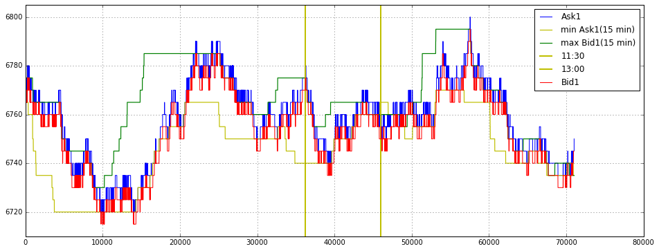
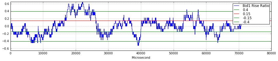
This block produces three stacked visualizations that together juxtapose the best bid/ask price series with short-term range markers and two compact momentum-like metrics. The overall intent — given the context of quantitative trading — is to make microstructure movements, intraday regime boundaries, and the intensity/direction of short-term moves easy to read so you can spot trade opportunities or regime changes.
First figure (price context). We start a wide figure and draw a grid to help read vertical relationships. Ask1_16 is plotted as the primary series (blue); Bid1_16 is added later (red), so you can directly compare the best ask and best bid over the same time axis. The code explicitly slices auxiliary series to the length of Ask1_16 — this enforces alignment: every overlaid line uses the same sample count so visual points correspond to the same time index. Two overlaid series represent short-window extrema: min15_Ask1_time_series (yellow) shows a rolling 15-minute minimum of the ask, and max_Bid1_time_series (green) shows a rolling 15-minute maximum of the bid. Plotting these extrema highlights the local short-term range and helps you see breakouts, mean-reversion windows, or widening/narrowing of spread dynamics that are useful when deciding entry/exit or sizing. Two vertical lines are drawn at index11_16 and index13_16 and labeled 11:30 and 13:00; these are session/time markers — useful for correlating price moves with scheduled events, session openings/closings, or intra-day regime shifts. Finally the y-range is clamped to (6710, 6805) to focus the view on the relevant price band and suppress distracting long tails; the legend is turned on to keep the plot interpretable.
Second and third figures (short-term directional intensity). Each of the next two narrow figures displays a “rise ratio” for asks and bids respectively. These rise_ratio_* arrays are plotted as compact blue lines with grid and tighter vertical scale; while the code doesn’t show their computation, the name and usage imply they are normalized measures of recent upward movement (e.g., fractional change, z-score, or slope over a short window). Normalizing or turning raw changes into a ratio is important in quant trading because it lets you compare signal strength across different price regimes and instruments and avoid false triggers when absolute price movement magnitude varies. The plots include horizontal threshold lines at ±0.15 and ±0.4 (and a 0.15 line colored red) — these act as visual decision boundaries: the mid threshold likely represents a moderate signal (possible trade or caution), while the outer threshold flags a strong move or breakout. Using symmetric positive and negative thresholds is purposeful: it makes it straightforward to detect strong buying pressure (positive exceedance) versus strong selling pressure (negative exceedance). Both plots limit the y-axis to ±0.65 so those thresholds are always visible and comparable across time.
import pandas as pd
import time
import csv
def order_book_tranform(year,month,day,path,best_price_number,series):
## read file
def read_file(year,month,day,path,series):
data = []
if len(str(month)) == 1:
month_ = ‘0’ + str(month)
else:
month_ = str(month)
if len(str(day)) == 1:
day_ = ‘0’ + str(day)
else:
day_ = str(day)
datapath = str(path) + str(year) + ‘.’ + str(month_) + ‘.’ + str(day_) + ‘.csv’
data = pd.read_csv(datapath)
data = data[data.Series == series]
return data.reset_index(drop = True)
def insert(order_book_data,data_to_insert,ob_position):
top = order_book_data[0:ob_position]
bottom = order_book_data[ob_position:]
return pd.concat((top,data_to_insert,bottom)).reset_index(drop = True)
def draw_out(order_book_data,ob_position):
top = order_book_data[0:ob_position]
bottom = order_book_data[ob_position + 1:]
return pd.concat((top,bottom)).reset_index(drop = True)
def order_book_to_csv(order_book_bid,order_book_ask,data,i):
order_book_bid_sum = order_book_bid[[’Price’,’QuantityDifference’]].groupby(by = [’Price’],as_index = False,sort = False).sum()
order_book_ask_sum = order_book_ask[[’Price’,’QuantityDifference’]].groupby(by = [’Price’],as_index = False).sum()
order_book_bid_sum = order_book_bid_sum[order_book_bid_sum.QuantityDifference != 0.0].reset_index(drop = True)
order_book_ask_sum = order_book_ask_sum[order_book_ask_sum.QuantityDifference != 0.0].reset_index(drop = True)
order_book_bid_ask = pd.concat([order_book_bid_sum[[’Price’,’QuantityDifference’]],order_book_ask_sum[[’Price’,’QuantityDifference’]]],axis = 1)
with open(’order_book_’+str(best_price_number)+’_’+str(year)+’_’+str(month)+’_’+str(day)+’.csv’,’a’) as f:
order_book = csv.writer(f)
order_book.writerow([”TimeStamp”,data.TimeStamp[i-1:i].iloc[0]])
order_book = csv.writer(f,delimiter=’,’)
for i in range(0,min(len(order_book_bid_ask),best_price_number),1):
order_book.writerow(order_book_bid_ask[i:i+1].values.tolist()[0])
return order_book_bid_sum,order_book_ask_sum
data = read_file(year,month,day,path,series)
with open(’order_book_’ + str(best_price_number) + ‘_’ + str(year) + ‘_’ + str(month) + ‘_’ + str(day) + ‘.csv’, ‘wb’) as csvfile:
f = csv.writer(csvfile)
data[[’QuantityDifference’]] = data[[’QuantityDifference’]].astype(float)
data[’QuantityDifference_’] = data[’QuantityDifference’]
data_ask = data[(data.BidOrAsk == ‘A’)].reset_index(drop=True)
data_bid = data[(data.BidOrAsk == ‘B’)].reset_index(drop=True)
order_book_bid = []
order_book_ask = []
x1 = data[(data.BidOrAsk == ‘A’)].TimeStamp.unique()
x2 = data[(data.BidOrAsk == ‘B’)].TimeStamp.unique()
temp_ask = 0
temp_bid = 0
def first_order_create(index_,data):
timestamp = data.TimeStamp.unique()[index_]
print ‘timestamp = %s’%(timestamp)
bid = []
ask = []
timestamp_ = []
index_find = data[data[’TimeStamp’].str.contains(timestamp)].index[-1]
y = data[:index_find + 1]
bid.append(y[(y.BidOrAsk == ‘B’)][[”Price”,”OrderNumber”,”QuantityDifference”,”QuantityDifference_”]]) # bid
ask.append(y[(y.BidOrAsk == ‘A’)][[”Price”,”OrderNumber”,”QuantityDifference”,”QuantityDifference_”]]) # ask
a = bid[0].sort([’Price’],ascending = [False])
b = ask[0].sort([’Price’],ascending = [True])
order_book_bid = a[a.QuantityDifference != 0].reset_index(drop = True)
order_book_ask = b[b.QuantityDifference != 0].reset_index(drop = True)
order_book_bid_sum = order_book_bid[[’Price’,’QuantityDifference’]].groupby(by = [’Price’],as_index = False,sort = False).sum()
order_book_ask_sum = order_book_ask[[’Price’,’QuantityDifference’]].groupby(by = [’Price’],as_index = False).sum()
if len(order_book_bid_sum[order_book_bid_sum.QuantityDifference == 0.0]) != 0 and len(order_book_ask_sum[order_book_ask_sum.QuantityDifference == 0.0]) != 0:
print ‘Exist Bid Ask Order Book Price = Zero’
price_bid_zero = order_book_bid_sum[order_book_bid_sum.QuantityDifference == 0.0][’Price’][0]
price_ask_zero = order_book_ask_sum[order_book_ask_sum.QuantityDifference == 0.0][’Price’][0]
order_book_bid = order_book_bid[order_book_bid.Price != price_bid_zero]
order_book_ask = order_book_ask[order_book_ask.Price != price_ask_zero]
elif len(order_book_bid_sum[order_book_bid_sum.QuantityDifference == 0.0]) != 0 and len(order_book_ask_sum[order_book_ask_sum.QuantityDifference == 0.0]) == 0:
print ‘Exist Bid Order Book Price = Zero’
price_bid_zero = order_book_bid_sum[order_book_bid_sum.QuantityDifference == 0.0][’Price’][0]
order_book_bid = order_book_bid[order_book_bid.Price != price_bid_zero]
elif len(order_book_bid_sum[order_book_bid_sum.QuantityDifference == 0.0]) == 0 and len(order_book_ask_sum[order_book_ask_sum.QuantityDifference == 0.0]) != 0:
print ‘Exist Ask Order Book Price = Zero’
price_ask_zero = order_book_ask_sum[order_book_ask_sum.QuantityDifference == 0.0][’Price’][0]
order_book_ask = order_book_ask[order_book_ask.Price != price_ask_zero]
order_book_bid_sum = order_book_bid_sum[order_book_bid_sum.QuantityDifference != 0].reset_index(drop = True)
order_book_ask_sum = order_book_ask_sum[order_book_ask_sum.QuantityDifference != 0].reset_index(drop = True)
order_book_bid_ask = pd.concat([order_book_bid_sum[[’Price’,’QuantityDifference’]],order_book_ask_sum[[’Price’,’QuantityDifference’]]],axis = 1)
return order_book_bid, order_book_ask, order_book_bid_ask, timestamp, y, index_find
def with_first_order_book(best_price_number,year,month,day,timestamp,order_book_bid_ask,index_):
with open(’order_book_’+str(best_price_number)+’_’+str(year)+’_’+str(month)+’_’+str(day)+’.csv’,’a’) as f:
order_book = csv.writer(f)
if index_ == 0:
order_book.writerow([”Bid”,”Bid_Quantity”,”Ask”,”Ask_Quantity”])
order_book.writerow([”TimeStamp”,timestamp])
order_book = csv.writer(f,delimiter=’,’)
for i in range(0,min(len(order_book_bid_ask),best_price_number),1):
order_book.writerow(order_book_bid_ask[i:i+1].values.tolist()[0])
first_order_book_data_lenth = 0
order_book_bid_time = 0
order_book_ask_time = 0
for time in range(0,1000,1):
index_ = time
order_book_bid, order_book_ask, order_book_bid_ask,\
timestamp, y, index_find = first_order_create(index_, data)
if len(order_book_bid) != 0 and len(order_book_ask) != 0:
with_first_order_book(best_price_number,year,month,day,timestamp,order_book_bid_ask,index_)
break
elif len(order_book_bid) == 0 and len(order_book_ask) != 0:
with_first_order_book(best_price_number,year,month,day,timestamp,order_book_bid_ask,index_)
temp_ask +=1
elif len(order_book_bid) != 0 and len(order_book_ask) == 0:
with_first_order_book(best_price_number,year,month,day,timestamp,order_book_bid_ask,index_)
temp_bid +=1
print ‘-------------------------------------------’
print ‘index_find = %s’%(index_find)
for i in range(index_find + 1,100,1):#len(data), 1):
#print ‘---------------------------------’
#print data[[’Price’,’QuantityDifference’,’BidOrAsk’,’TimeStamp’]][i:i+1]
#print i ,temp_bid, temp_ask
#print data.TimeStamp[i], x2[temp_bid], x1[temp_ask]
time_second = int(data[i:i+1].TimeStamp.iloc[0][18]) + int(data[i:i+1].TimeStamp.iloc[0][17])*10 +\
int(data[i:i+1].TimeStamp.iloc[0][15])*60 + int(data[i:i+1].TimeStamp.iloc[0][14])*600 +\
int(data[i:i+1].TimeStamp.iloc[0][12])*3600 + int(data[i:i+1].TimeStamp.iloc[0][11])*36000
if time_second > 57600:
break
if time_second == 32400 and time_second >= 57300:
order_book_bid = order_book_bid.sort([’Price’],ascending = [False]).reset_index(drop = True)
order_book_ask = order_book_ask.sort([’Price’],ascending = [True]).reset_index(drop = True)
pass
if data.BidOrAsk[i] == ‘A’:
data_ask_Quantity = data.BestQuantity[i]
if int(data[[’QuantityDifference’]][i:i+1].values) > 0 :
if order_book_bid.Price[0] >= data[i:i+1].Price.iloc[0] and time_second < 32400:
for k in range(0,len(order_book_bid)):
diff = order_book_bid.QuantityDifference_[k] - data[i:i+1].QuantityDifference_.iloc[0]
if order_book_bid.Price[k] >= data[i:i+1].Price.iloc[0] and diff >= 0:
order_book_bid.QuantityDifference_[k] = diff
data[i:i+1].QuantityDifference_.iloc[0] = 0
break
elif order_book_bid.Price[k] >= data[i:i+1].Price.iloc[0] and diff < 0:
order_book_bid.QuantityDifference_[k] = 0
data[i:i+1].QuantityDifference_.iloc[0] = -diff
pass
else:
break
if data.TimeStamp[i] == x1[temp_ask]:
position_ = int(data[[’OrderBookPosition’]][i:i+1].iloc[0]) - 1
order_book_ask = insert(order_book_ask,data[[’Price’,’OrderNumber’,’QuantityDifference’,’QuantityDifference_’]][i:i+1],position_)
if time_second > 32400 and time_second < 57300:
if position_ == 0 and len(order_book_ask) > 1:
if order_book_ask[position_ + 1:position_ + 1 + 1][”Price”].iloc[0] < data[’Price’][i:i+1].iloc[0]:
print ‘Some error1(Ask & Q>0 & timestamp not change & 1),position = %d,index = %d,price = %d,OrderNumber = %s’%(position_,i,data[’Price’][i:i+1].iloc[0],data[’OrderNumber’][i:i+1].iloc[0])
break
else:
pass
elif 0 < position_< (len(order_book_ask)-1):
if order_book_ask[position_ + 1:position_+1+1][”Price”].iloc[0] < data[’Price’][i:i+1].iloc[0] or order_book_ask[position_ - 1:position_ - 1 + 1][”Price”].iloc[0] > data[’Price’][i:i+1].iloc[0]:
print ‘Some error1(Ask & Q>0 & timestamp not change & 2),position = %d,index = %d,price = %d,OrderNumber = %s’%(position_,i,data[’Price’][i:i+1].iloc[0],data[’OrderNumber’][i:i+1].iloc[0])
break
else:
pass
elif position_ == len(order_book_ask)-1:
if order_book_ask[position_ - 1:position_ - 1 + 1][”Price”].iloc[0] > data[’Price’][i:i+1].iloc[0]:
print ‘Some error1(Ask & Q>0 & timestamp not change & 3),position = %d,index = %d,price = %d,OrderNumber = %s’%(position_,i,data[’Price’][i:i+1].iloc[0],data[’OrderNumber’][i:i+1].iloc[0])
break
else:
pass
elif position_ == 0 and len(order_book_ask) == 1:
pass
else:
pass
elif data.TimeStamp[i] != x1[temp_ask]:
if temp_ask == 0:
temp_ask = temp_ask + 1
best_price = data[i:(i+1)][’BestPrice’]
position_ = int(data[[’OrderBookPosition’]][i:i+1].iloc[0]) - 1
order_book_ask = insert(order_book_ask,data[[’Price’,’OrderNumber’,’QuantityDifference’,’QuantityDifference_’]][i:i+1],position_)
if time_second > 32400 and time_second < 57300:
if position_ == 0 and len(order_book_ask) > 1:
if order_book_ask[position_+1:position_+1+1][”Price”].iloc[0] < data[’Price’][i:i+1].iloc[0]:
print ‘Some error2(Ask & Q>0 & timestamp change & 1),position = %d,index = %d,price = %d,OrderNumber = %s’%(position_,i,data[’Price’][i:i+1].iloc[0],data[’OrderNumber’][i:i+1].iloc[0])
break
else:
pass
elif 0 < position_< len(order_book_ask)-1:
if order_book_ask[position_+ 1:position_+1+1][”Price”].iloc[0] < data[’Price’][i:i+1].iloc[0] or order_book_ask[position_-1:position_-1+1][”Price”].iloc[0] > data[’Price’][i:i+1].iloc[0]:
print ‘Some error2(Ask & Q>0 & timestamp change & 2),position = %d,index = %d,price = %d,OrderNumber = %s’%(position_,i,data[’Price’][i:i+1].iloc[0],data[’OrderNumber’][i:i+1].iloc[0])
break
else:
pass
elif position_ == len(order_book_ask)-1:
if order_book_ask[position_-1:position_-1+1][”Price”].iloc[0] > data[’Price’][i:i+1].iloc[0]:
print ‘Some error2(Ask & Q>0 & timestamp change & 3),position = %d,index = %d,price = %d,OrderNumber = %s’%(position_,i,data[’Price’][i:i+1].iloc[0],data[’OrderNumber’][i:i+1].iloc[0])
break
else:
pass
elif position_ == 0 and len(order_book_ask) == 1:
pass
else:
pass
else:
order_book_bid_sum,order_book_ask_sum = order_book_to_csv(order_book_bid,order_book_ask,data,i)
if time_second > 32400 and time_second < 57300:
if round(float(data[i:i+1].TimeStamp.iloc[0][18:29]) - float(data[i-1:i].TimeStamp.iloc[0][18:28]),4) > 0.03 or\
round(float(data[i:i+1].TimeStamp.iloc[0][18:29]) - float(data[i-1:i].TimeStamp.iloc[0][18:28]),4) < 0:
if data[i-1:i].BidOrAsk.iloc[0] == ‘A’:
if order_book_ask_sum[0:1].values.tolist()[0][1] == data[i-1:i].BestQuantity.iloc[0]:
pass
else:
print ‘Best ask quantity is false’
pass
#break
else:
j = i - 1
while j >= 1:
if data[j-1:j].BidOrAsk.iloc[0] == ‘A’:
if order_book_ask_sum[0:1].values.tolist()[0][1] == data[j-1:j].BestQuantity.iloc[0]:
break
else:
j = j - 1
pass
else:
pass
else:
pass
position_ = int(data[[’OrderBookPosition’]][i:i+1].iloc[0]) - 1
temp_ask = temp_ask + 1
order_book_ask = insert(order_book_ask,data[[’Price’,’OrderNumber’,’QuantityDifference’,’QuantityDifference_’]][i:i+1],position_)
if time_second > 32400 and time_second < 57300:
if position_ == 0:
if order_book_ask[position_+1:position_+1+1][”Price”].iloc[0] < data[’Price’][i:i+1].iloc[0]:
print ‘Some error3(Ask & Q>0 & timestamp change & 1),position = %d,index = %d,price = %d,OrderNumber = %s’%(position_,i,data[’Price’][i:i+1].iloc[0],data[’OrderNumber’][i:i+1].iloc[0])
break
else:
pass
elif 0 < position_< len(order_book_ask)-1:
if order_book_ask[position_+1:position_+1+1][”Price”].iloc[0] < data[’Price’][i:i+1].iloc[0]:
print ‘Some error3(Ask & Q>0 & timestamp change & 2),position = %d,index = %d,price = %d,OrderNumber = %s’%(position_,i,data[’Price’][i:i+1].iloc[0],data[’OrderNumber’][i:i+1].iloc[0])
break
else:
pass
elif position_ == len(order_book_ask)-1:
if order_book_ask[position_-1:position_-1+1][”Price”].iloc[0] > data[’Price’][i:i+1].iloc[0]:
print ‘Some error3(Ask & Q>0 & timestamp change & 3),position = %d,index = %d,price = %d,OrderNumber = %s’%(position_,i,data[’Price’][i:i+1].iloc[0],data[’OrderNumber’][i:i+1].iloc[0])
break
else:
pass
elif position_ == 0 and len(order_book_ask[0]) == 1:
pass
else:
pass
elif int(data[[’QuantityDifference’]][i:i+1].values) < 0:
if data.TimeStamp[i] == x1[temp_ask]:
order_number_ = data[’OrderNumber’][i:i + 1].iloc[0]
position_ = order_book_ask[order_book_ask.OrderNumber == order_number_].index[0]
price_ = data[i:i+1][’Price’].iloc[0]
if time_second > 32400 and time_second < 57300:
if position_ == 0 and len(order_book_ask) > 1:
if order_book_ask[position_+1:position_+1+1][”Price”].iloc[0] < data[’Price’][i:i+1].iloc[0]:
print ‘Some error4(Ask & Q<0 & timestamp not change & 1),position = %d,index = %d,price = %d,OrderNumber = %s’%(position_,i,data[’Price’][i:i+1].iloc[0],data[’OrderNumber’][i:i+1].iloc[0])
break
else:
pass
elif 0 < position_< len(order_book_ask)-1:
if order_book_ask[position_+1:position_+1+1][”Price”].iloc[0] < data[’Price’][i:i+1].iloc[0]:
print ‘Some error4(Ask & Q<0 & timestamp not change & 2),position = %d,index = %d,price = %d,OrderNumber = %s’%(position_,i,data[’Price’][i:i+1].iloc[0],data[’OrderNumber’][i:i+1].iloc[0])
break
else:
pass
elif position_ == len(order_book_ask)-1:
if position_ > 0 and order_book_ask[position_-1:position_-1+1][”Price”].iloc[0] > data[’Price’][i:i+1].iloc[0]:
print ‘Some error4(Ask & Q<0 & timestamp not change & 3),position = %d,index = %d,price = %d,OrderNumber = %s’%(position_,i,data[’Price’][i:i+1].iloc[0],data[’OrderNumber’][i:i+1].iloc[0])
break
elif position_ == 0:
pass
else:
pass
elif position_ == 0 and len(order_book_ask) == 1:
pass
else:
pass
if order_book_ask[(order_book_ask.OrderNumber == order_number_)&(order_book_ask.Price == price_)][’QuantityDifference’].iloc[0] == abs(data[i:i+1][’QuantityDifference’].iloc[0]):
order_book_ask = order_book_ask.drop(order_book_ask.index[[position_]]).reset_index(drop = True)
else:
order_book_ask[’QuantityDifference’][order_book_ask.OrderNumber == order_number_] = order_book_ask[’QuantityDifference’][order_book_ask.OrderNumber == order_number_] + data[i:i+1][’QuantityDifference’].iloc[0]
elif data.TimeStamp[i] != x1[temp_ask]:
order_book_bid_sum,order_book_ask_sum = order_book_to_csv(order_book_bid,order_book_ask,data,i)
if time_second > 32400 and time_second < 57300:
if round(float(data[i:i+1].TimeStamp.iloc[0][18:29]) - float(data[i-1:i].TimeStamp.iloc[0][18:28]),4) > 0.03 or\
round(float(data[i:i+1].TimeStamp.iloc[0][18:29]) - float(data[i-1:i].TimeStamp.iloc[0][18:28]),4) < 0:
if data[i-1:i].BidOrAsk.iloc[0] == ‘A’:
if order_book_ask_sum[0:1].values.tolist()[0][1] == data[i-1:i].BestQuantity.iloc[0]:
pass
else:
print ‘Best ask quantity is false’
#break
pass
else:
j = i - 1
while j >= 1:
if data[j-1:j].BidOrAsk.iloc[0] == ‘A’:
if order_book_ask_sum[0:1].values.tolist()[0][1] == data[j-1:j].BestQuantity.iloc[0]:
break
else:
j = j - 1
pass
else:
pass
order_number_ = data[’OrderNumber’][i : i + 1].iloc[0]
position_ = order_book_ask[order_book_ask.OrderNumber == order_number_].index[0]
price_ = data[i:i+1][’Price’].iloc[0]
temp_ask = temp_ask + 1
if time_second > 32400 and time_second < 57300:
if position_ == 0 and len(order_book_ask) > 1:
if order_book_ask[position_ + 1:position_+1+1][”Price”].iloc[0] < data[’Price’][i:i+1].iloc[0]:
print ‘Some error5(Ask & Q<0 & timestamp change & 1),position = %d,index = %d,price = %d,OrderNumber = %s’%(position_,i,data[’Price’][i:i+1].iloc[0],data[’OrderNumber’][i:i+1].iloc[0])
break
else:
pass
elif 0 < position_< len(order_book_ask)-1:
if order_book_ask[position_ + 1:position_+1+1][”Price”].iloc[0] < data[’Price’][i:i+1].iloc[0]:
print ‘Some error5(Ask & Q<0 & timestamp change & 2),position = %d,index = %d,price = %d,OrderNumber = %s’%(position_,i,data[’Price’][i:i+1].iloc[0],data[’OrderNumber’][i:i+1].iloc[0])
break
else:
pass
elif position_ == len(order_book_ask)-1:
if position_ > 0 and order_book_ask[position_-1:position_-1 + 1][”Price”].iloc[0] > data[’Price’][i:i+1].iloc[0]:
print ‘Some error5(Ask & Q<0 & timestamp change & 3),position = %d,index = %d,price = %d,OrderNumber = %s’%(position_,i,data[’Price’][i:i+1].iloc[0],data[’OrderNumber’][i:i+1].iloc[0])
break
elif position_ == 0:
pass
else:
pass
elif position_ == 0 and len(order_book_ask) == 1:
pass
else:
pass
if order_book_ask[(order_book_ask.OrderNumber == order_number_)&(order_book_ask.Price == price_)][’QuantityDifference’].iloc[0] == abs(data[i:i+1][’QuantityDifference’].iloc[0]):
order_book_ask = order_book_ask.drop(order_book_ask.index[[position_]]).reset_index(drop = True)
else:
order_book_ask[’QuantityDifference’][order_book_ask.OrderNumber == order_number_] = order_book_ask[’QuantityDifference’][order_book_ask.OrderNumber == order_number_] + data[i:i+1][’QuantityDifference’].iloc[0]
elif data.BidOrAsk[i] == ‘B’:
data_bid_Quantity = data.BestQuantity[i]
if int(data[[’QuantityDifference’]][i:i+1].values) > 0:
if order_book_ask.Price[0] <= data[i:i+1].Price.iloc[0] and time_second < 32400:
for k in range(0,len(order_book_ask)):
diff = order_book_ask.QuantityDifference_[k] - data[i:i+1].QuantityDifference_.iloc[0]
if order_book_ask.Price[k] <= data[i:i+1].Price.iloc[0] and diff >= 0:
order_book_ask.QuantityDifference_[k] = diff
data[i:i+1].QuantityDifference_.iloc[0] = 0
break
elif order_book_ask.Price[k] <= data[i:i+1].Price.iloc[0] and diff < 0:
order_book_ask.QuantityDifference_[k] = 0
data[i:i+1].QuantityDifference_.iloc[0] = - diff
pass
else:
break
if data.TimeStamp[i] == x2[temp_bid]:
position_ = int(data[[’OrderBookPosition’]][i:i+1].iloc[0]) - 1
order_book_bid = insert(order_book_bid,data[[’Price’,’OrderNumber’,’QuantityDifference’,’QuantityDifference_’]][i:i+1],position_)
if time_second > 32400 and time_second < 57300:
if position_ == 0 and len(order_book_bid) > 1:
if order_book_bid[position_+1:position_+1+1][”Price”].iloc[0] > data[’Price’][i:i+1].iloc[0]:
print ‘Some error1(Bid & Q>0 & timestamp not change & 1),position = %d,index = %d,price = %d,OrderNumber = %s’%(position_,i,data[’Price’][i:i+1].iloc[0],data[’OrderNumber’][i:i+1].iloc[0])
break
else:
pass
elif 0 < position_< len(order_book_bid)-1:
if order_book_bid[position_-1:position_-1+1][”Price”].iloc[0] < data[’Price’][i:i+1].iloc[0] or order_book_bid[position_+1:position_+1+1][”Price”].iloc[0] > data[’Price’][i:i+1].iloc[0]:
print ‘Some error1(Bid & Q>0 & timestamp not change & 2),position = %d,index = %d,price = %d,OrderNumber = %s’%(position_,i,data[’Price’][i:i+1].iloc[0],data[’OrderNumber’][i:i+1].iloc[0])
break
else:
pass
elif position_ == len(order_book_bid)-1 and len(order_book_bid) > 1:
if order_book_bid[position_-1:position_-1+1][”Price”].iloc[0] < data[’Price’][i:i+1].iloc[0]:
print ‘Some error1(Bid & Q>0 & timestamp not change & 3),position = %d,index = %d,price = %d,OrderNumber = %s’%(position_,i,data[’Price’][i:i+1].iloc[0],data[’OrderNumber’][i:i+1].iloc[0])
break
else:
pass
elif position_ == 0 and len(order_book_bid[temp_bid]) == 1:
pass
else:
pass
elif data.TimeStamp[i] != x2[temp_bid]:
if temp_bid == 0:
best_price = data[i:(i+1)][’BestPrice’]
position_ = int(data[[’OrderBookPosition’]][i:i+1].iloc[0]) - 1
temp_bid = temp_bid + 1
order_book_bid = insert(order_book_bid,data[[’Price’,’OrderNumber’,’QuantityDifference’,’QuantityDifference_’]][i:i+1],position_)
if time_second > 32400 and time_second < 57300:
if position_ == 0 and len(order_book_bid) > 1:
if order_book_bid[position_+1:position_+1+1][”Price”].iloc[0] > data[’Price’][i:i+1].iloc[0] or order_book_bid[’Price’][0:1].iloc[0] != data[’BestPrice’][i]:
print ‘Some error2(Bid & Q>0 & timestamp change & 1),position = %d,index = %d,price = %d,OrderNumber = %s’%(position_,i,data[’Price’][i:i+1].iloc[0]) + data[’OrderNumber’][i:i+1].iloc[0]
break
else:
pass
elif 0 < position_< len(order_book_bid)-1:
if order_book_bid[position_-1:position_-1+1][”Price”].iloc[0] < data[’Price’][i:i+1].iloc[0] or order_book_bid[position_+1:position_+1+1][”Price”].iloc[0] > data[’Price’][i:i+1].iloc[0]:
print ‘Some error2(Bid & Q>0 & timestamp change & 2),position = %d,index = %d,price = %d,OrderNumber = %s’%(position_,i,data[’Price’][i:i+1].iloc[0],data[’OrderNumber’][i:i+1].iloc[0])
break
else:
pass
elif position_ == len(order_book_bid)-1:
if order_book_bid[position_-1:position_-1+1][”Price”].iloc[0] < data[’Price’][i:i+1].iloc[0] or order_book_bid[’Price’][0:1].iloc[0] != data[’BestPrice’][i]:
print ‘Some error2(Bid & Q>0 & timestamp change & 3),position = %d,index = %d,price = %d,OrderNumber = %s’%(position_,i,data[’Price’][i:i+1].iloc[0],data[’OrderNumber’][i:i+1].iloc[0])
pass
else:
pass
elif position_ == 0 and len(order_book_bid) == 1:
pass
else:
pass
else:
if time_second > 32400 and time_second < 57300:
if round(float(data[i:i+1].TimeStamp.iloc[0][18:29]) - float(data[i-1:i].TimeStamp.iloc[0][18:28]),4) > 0.03 or\
round(float(data[i:i+1].TimeStamp.iloc[0][18:29]) - float(data[i-1:i].TimeStamp.iloc[0][18:28]),4) < 0:
order_book_bid_sum,order_book_ask_sum = order_book_to_csv(order_book_bid,order_book_ask,data,i)
if data[i-1:i].BidOrAsk.iloc[0] == ‘B’:
if order_book_bid_sum[0:1].values.tolist()[0][1] == data[i-1:i].BestQuantity.iloc[0]:
pass
else:
print ‘Best bid quantity is false’
#break
pass
else:
j = i - 1
while j >= 1:
if data[j-1:j].BidOrAsk.iloc[0] == ‘B’:
if order_book_bid_sum[0:1].values.tolist()[0][1] == data[j-1:j].BestQuantity.iloc[0]:
break
else:
print ‘Best bid quantity is false’
#break
pass
else:
j = j - 1
pass
else:
pass
position_ = int(data[[’OrderBookPosition’]][i:i+1].iloc[0]) - 1
temp_bid = temp_bid + 1
order_book_bid = insert(order_book_bid,data[[’Price’,’OrderNumber’,’QuantityDifference’,’QuantityDifference_’]][i:i+1],position_)
if time_second > 32400 and time_second < 57300:
if position_ == 0 and len(order_book_bid) > 1:
if order_book_bid[position_+1:position_+1+1][”Price”].iloc[0] > data[’Price’][i:i+1].iloc[0] or order_book_bid[’Price’][0:1].iloc[0] != data[’BestPrice’][i]:
print ‘Some error3(Bid & Q>0 & timestamp change & 1),position = %d,index = %d,price = %d,OrderNumber = %s’%(position_,i,data[’Price’][i:i+1].iloc[0],data[’OrderNumber’][i:i+1].iloc[0])
break
else:
pass
elif 0 < position_< len(order_book_bid)-1:
if order_book_bid[position_-1:position_-1+1][”Price”].iloc[0] < data[’Price’][i:i+1].iloc[0] or order_book_bid[position_+1:position_+1+1][”Price”].iloc[0] > data[’Price’][i:i+1].iloc[0]:
print ‘Some error3(Bid & Q>0 & timestamp change & 2),position = %d,index = %d,price = %d,OrderNumber = %s’%(position_,i,data[’Price’][i:i+1].iloc[0],data[’OrderNumber’][i:i+1].iloc[0])
break
else:
pass
elif position_ == len(order_book_bid)-1:
if order_book_bid[position_-1:position_-1 + 1][”Price”].iloc[0] < data[’Price’][i:i+1].iloc[0] or order_book_bid[’Price’][0:1].iloc[0] != data[’BestPrice’][i]:
print ‘Some error3(Bid & Q>0 & timestamp change & 3),position = %d,index = %d,price = %d,OrderNumber = %s’%(position_,i,data[’Price’][i:i+1].iloc[0],data[’OrderNumber’][i:i+1].iloc[0])
break
else:
pass
elif position_ == 0 and len(order_book_bid[0]) == 1:
pass
else:
pass
elif int(data[[’QuantityDifference’]][i:i+1].values) < 0:
if data.TimeStamp[i] == x2[temp_bid]:
order_number_ = data[’OrderNumber’][i : i + 1].iloc[0]
position_ = order_book_bid[order_book_bid.OrderNumber == order_number_].index[0]
price_ = data[i:i+1][’Price’].iloc[0]
if time_second > 32400 and time_second < 57300:
if position_ == 0 and len(order_book_bid) > 1:
if order_book_bid[position_+1:position_+1+1][”Price”].iloc[0] > data[’Price’][i:i+1].iloc[0]:
print ‘Some error4(Bid & Q<0 & timestamp not change & 1),position = %d,index = %d,price = %d,OrderNumber = %s’%(position_,i,data[’Price’][i:i+1].iloc[0],data[’OrderNumber’][i:i+1].iloc[0])
break
else:
pass
elif 0 < position_< len(order_book_bid)-1:
if order_book_bid[position_-1:position_-1+1][”Price”].iloc[0] < data[’Price’][i:i+1].iloc[0] or order_book_bid[position_+1:position_+1+1][”Price”].iloc[0] > data[’Price’][i:i+1].iloc[0]:
print ‘Some error4(Bid & Q<0 & timestamp not change & 2),position = %d,index = %d,price = %d,OrderNumber = %s’%(position_,i,data[’Price’][i:i+1].iloc[0],data[’OrderNumber’][i:i+1].iloc[0])
break
else:
pass
elif position_ == len(order_book_bid)-1:
if order_book_bid[position_-1:position_-1+1][”Price”].iloc[0] < data[’Price’][i:i+1].iloc[0]:
print ‘Some error4(Bid & Q<0 & timestamp not change & 3),position = %d,index = %d,price = %d,OrderNumber = %s’%(position_,i,data[’Price’][i:i+1].iloc[0],data[’OrderNumber’][i:i+1].iloc[0])
break
elif position_ == 0:
pass
else:
pass
elif position_ == 0 and len(order_book_bid) == 1:
pass
else:
pass
if order_book_bid[(order_book_bid.OrderNumber == order_number_)&(order_book_bid.Price == price_)][’QuantityDifference’].iloc[0] == abs(data[i:i+1][’QuantityDifference’].iloc[0]):
order_book_bid = order_book_bid.drop(order_book_bid.index[[position_]]).reset_index(drop = True)
else:
order_book_bid[’QuantityDifference’][order_book_bid.OrderNumber == order_number_] = order_book_bid[’QuantityDifference’][order_book_bid.OrderNumber == order_number_] + data[i:i+1][’QuantityDifference’].iloc[0]
elif data.TimeStamp[i] != x2[temp_bid]:
if time_second > 32400 and time_second < 57300:
if round(float(data[i:i+1].TimeStamp.iloc[0][18:29]) - float(data[i-1:i].TimeStamp.iloc[0][18:28]),4) > 0.03 or\
round(float(data[i:i+1].TimeStamp.iloc[0][18:29]) - float(data[i-1:i].TimeStamp.iloc[0][18:28]),4) < 0:
order_book_bid_sum,order_book_ask_sum = order_book_to_csv(order_book_bid,order_book_ask,data,i)
if data[i-1:i].BidOrAsk.iloc[0] == ‘B’:
if order_book_bid_sum[0:1].values.tolist()[0][1] == data[i-1:i].BestQuantity.iloc[0]:
pass
else:
print ‘Best bid quantity is false’
#break
pass
else:
j = i - 1
while j >= 1:
if data[j-1:j].BidOrAsk.iloc[0] == ‘B’:
if order_book_bid_sum[0:1].values.tolist()[0][1] == data[j-1:j].BestQuantity.iloc[0]:
break
else:
print ‘Best bid quantity is false’
#break
pass
else:
j = j - 1
pass
else:
pass
order_number_ = data[’OrderNumber’][i:i+1].iloc[0]
position_ = order_book_bid[order_book_bid.OrderNumber == order_number_].index[0]
price_ = data[i:i+1][’Price’].iloc[0]
temp_bid = temp_bid + 1
if time_second > 32400 and time_second < 57300:
if position_ == 0 and len(order_book_bid) > 1:
if order_book_bid[position_+1:position_+1+1][”Price”].iloc[0] > data[’Price’][i:i+1].iloc[0]:
print ‘Some error5(Bid & Q<0 & timestamp change & 1),position = %d,index = %d,price = %d,OrderNumber = %s’%(position_,i,data[’Price’][i:i+1].iloc[0],data[’OrderNumber’][i:i+1].iloc[0])
break
else:
pass
elif 0 < position_< len(order_book_bid)-1:
if order_book_bid[position_-1:position_-1+1][”Price”].iloc[0] < data[’Price’][i:i+1].iloc[0] or order_book_bid[position_+1:position_+1+1][”Price”].iloc[0] > data[’Price’][i:i+1].iloc[0]:
print ‘Some error5(Bid & Q<0 & timestamp change & 2),position = %d,index = %d,price = %d,OrderNumber = %s’%(position_,i,data[’Price’][i:i+1].iloc[0],data[’OrderNumber’][i:i+1].iloc[0])
break
else:
pass
elif position_ == len(order_book_bid)-1:
if order_book_bid[position_-1:position_-1+1][”Price”].iloc[0] < data[’Price’][i:i+1].iloc[0]:
print ‘Some error5(Bid & Q<0 & timestamp change & 3),position = %d,index = %d,price = %d,OrderNumber = %s’%(position_,i,data[’Price’][i:i+1].iloc[0],data[’OrderNumber’][i:i+1].iloc[0])
break
elif position_ == 0:
pass
else:
pass
elif position_ == 0 and len(order_book_bid) == 1:
pass
else:
pass
if order_book_bid[(order_book_bid.OrderNumber == order_number_)&(order_book_bid.Price == price_)][’QuantityDifference’].iloc[0] == abs(data[i:i+1][’QuantityDifference’].iloc[0]):
order_book_bid = order_book_bid.drop(order_book_bid.index[[position_]]).reset_index(drop = True)
else:
order_book_bid[’QuantityDifference’][order_book_bid.OrderNumber == order_number_] = order_book_bid[’QuantityDifference’][order_book_bid.OrderNumber == order_number_] + data[i:i+1][’QuantityDifference’].iloc[0]
return data, order_book_bid, order_book_ask #, order_book_bid_sum, order_book_ask_sum
if __name__ == ‘__main__’:
path = ‘/home/rory/Demo/Data_Transformation/message_data/CN_Futures_’
year = 2014
best_price_number = 3
series = ‘CNF14’
month = 1
day_ = [2]
for i in day_:
print i
start = time.time()
data, order_book_bid, order_book_ask = order_book_tranform(year,month,i,path,best_price_number,series)
end = time.time()
print “Total time = %f”%(end - start)
Goal and high-level flow: This routine reconstructs a limit order book from a sequence of exchange message records and emits periodic top-of-book snapshots (best N price levels) to a CSV. In a quant-trading workflow we need an accurate LOB (limit order book) reconstruction from message-level data so we can compute microstructure features (spread, depth, liquidity consumption) and validate recorded “best” fields in the tape. The code reads the raw message CSV for a specific contract (series) and then walks events in chronological order, applying each message to an in-memory bid and ask book representation, emitting aggregated snapshots when timestamps change or when certain conditions are met.
File reading and initial preparation: The helper read_file builds the file path for the given date and loads only rows for the requested series. Immediately after loading, the code coerces QuantityDifference to float and makes a copy QuantityDifference_ — this second column is used so the algorithm can mutate a working quantity during matching (subtracting partial fills) while still having the original quantity if needed for other logic or validations. The dataset is also split into data_bid/data_ask filtered by the BidOrAsk flag; unique timestamps for ask and bid messages are computed into x1/x2 and two counters temp_ask/temp_bid are initialized to track timestamp boundaries as the code progresses.
Constructing the initial order book: The first_order_create inner function tries to build an initial snapshot by taking all messages up to the last row of a chosen timestamp and aggregating all outstanding orders at that moment. It extracts rows for Bid (B) and Ask (A), sorts bids descending by price and asks ascending by price, and groups by price to sum quantities — this produces the level-aggregated view (quantity per price). It then drops any price levels whose net QuantityDifference sums to zero (these are fully cancelled/executed). The outer loop calls first_order_create over timestamps (up to 1000 attempts) until it finds a moment when both bid and ask books are non-empty; that moment becomes the starting book and is written to CSV (the helper with_first_order_book writes a header and then the top-best_price_number rows). This initialization guarantees we start simulation from a valid LOB state (both sides present) rather than an empty or one-sided book.
Event-by-event processing (main loop): After the index_find that defined the initial snapshot, the main loop iterates forward through message events. For each message it computes a time_second integer by slicing the TimeStamp string and converting hour/minute/second digits to seconds-of-day; this is used to stop processing after the exchange end (a hard break if > 57600) and to enable different behavior inside vs outside core trading hours (the code treats seconds < 32400, between 32400 and 57300, and beyond differently). Each event’s behavior depends on BidOrAsk and the sign of QuantityDifference:
- Additions (QuantityDifference > 0): An incoming “add” may be a passive limit order that just joins the book, or a marketable/aggressive order that immediately matches existing opposite-side liquidity. The code first checks for immediate matching with the opposite book top-of-book price (for example, an incoming Ask add that is priced at or below the best bid). If it is marketable and pre-open (or for some time condition, the code uses time_second < 32400), it walks through the opposite book levels subtracting quantities from order_book_* .QuantityDifference_ until the incoming quantity is exhausted or no more price-compatible levels exist — this implements basic matching/consumption logic and updates the remaining QuantityDifference_ on levels and the incoming message.
If the incoming order remains (or was passive to start), the code inserts it into the local order_book_ask/bid list at the index given by the incoming message’s OrderBookPosition (the insert helper performs a top/bottom split and concatenation). When the message timestamp is a boundary (i.e., the message timestamp differs from the last timestamp for that side), the code writes the current aggregated book to CSV by grouping quantities by price via order_book_to_csv and performs validation checks: in core hours it compares the computed best-level aggregated quantity with the data’s BestQuantity field to detect mismatches.
- Reductions/cancels/trades (QuantityDifference < 0): For decreases the code locates the order to be reduced by matching OrderNumber and Price to find its position in the local book. If the reduction exactly matches the outstanding level quantity, the row is dropped; otherwise the QuantityDifference on that order is updated by adding the negative delta (i.e., reducing the stored quantity). When the timestamp changes between messages, the code likewise aggregates and writes the top-N snapshot and runs the same best-quantity consistency checks.
Aggregation and writing snapshots: The order_book_to_csv helper first groups the internal order lists by Price and sums QuantityDifference so the output is a price-level aggregated book (this is what most quant features use: depth at price levels). It filters out zero-quantity levels, concatenates bid and ask side frames into a single row-wise view, writes the timestamp row and then writes up to best_price_number rows to the CSV. This design keeps disk output compact (price-level aggregation) and generates time-stamped snapshots aligned with observed message timestamps so downstream models can compute features like mid, spread and depth time series.
Validation and defensive checks: Throughout the event handling there are many conditional checks (the “Some errorX” prints) that assert local invariants: that inserted orders have prices consistent with neighbouring levels, that position indices make sense relative to sorting order, and that during core trading hours best-level aggregated quantities match the BestQuantity reported in the input. These checks are important for two reasons in quant trading: they surface data-feed inconsistencies early (helping distinguish replay vs tape mismatches) and they protect against logic errors in reconstructing order positions from OrderBookPosition fields. When these checks fail the code prints diagnostic context (position, index, price, OrderNumber) and in many cases breaks execution.
Implementation notes that explain “why” of some choices: QuantityDifference_ is a working copy used to decrement order quantities as we simulate matching so the original QuantityDifference column remains available for comparisons; grouping by price before writing reduces noise from per-order granularity to the price-level book needed for most analytics. The code also uses timestamp changes as natural snapshot boundaries because many exchanges report best prices/quantities per message timestamp and you want snapshots aligned to those changes. The various time-second thresholds (32400, 57300, 57600) gate special treatment in the code (different validation strictness and an end-of-day break) to respect market session boundaries.
Outputs and return values: The function writes a CSV file named order_book_<best_price_number>_<year>_<month>_<day>.csv containing alternating timestamp rows and price-level rows for the aggregated top levels, and returns the original data plus the final in-memory order_book_bid and order_book_ask frames for further programmatic inspection.
pd.read_csv(’CN_Futures_2014.01.02.csv’).head(10)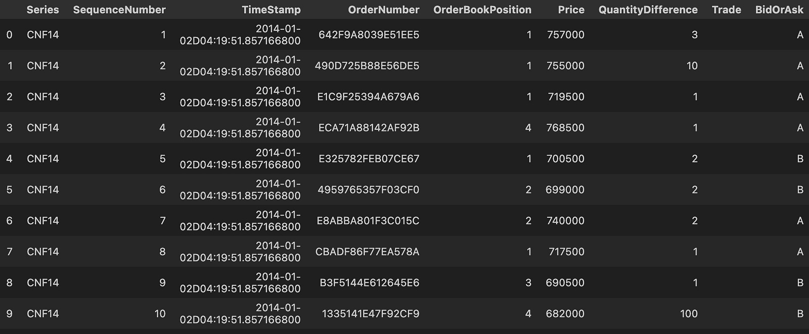
This one-liner is a quick, exploratory step in the data pipeline: pandas opens the CSV at the given path, interprets the file structure, materializes a DataFrame, and then returns the first ten rows for inspection. Conceptually the flow is: disk → parser → in-memory table → sample slice. We use head(10) here not because we want only ten rows saved, but because we want a fast sanity check of the file’s schema and values before committing to heavier processing. In other words, this line is about discovering what the message-level data looks like (column names, sample values, timestamp formats, numeric scales and missing-value markers) so we can design subsequent cleaning and transformation steps appropriately.
There are a few important consequences of how this is written that affect performance and correctness in a quant-trading context. By default read_csv will attempt to infer dtypes and will read the whole file into memory before head(10) extracts the sample; for large tick-message files this can be slow or OOM. If the intent is only to preview the file, prefer read_csv(…, nrows=10) to avoid loading the entire dataset. Conversely, if you actually want to load the whole trading day for downstream processing, you should explicitly control parsing (dtype, parse_dates, usecols, chunksize) so pandas doesn’t make lossy or inconsistent inferences that later harm numeric precision or sort order.
Why this inspection matters for the trading pipeline: message data for futures typically contains high-frequency timestamps, tick prices and sizes, and discrete message types (trades, quotes, cancels, etc.). If timestamps aren’t parsed to a precise datetime64[ns] (or you lose sub-second resolution), microstructure features and event ordering will be corrupted and backtests will be invalid. Similarly, automatic dtype inference can produce object dtypes for numeric-looking columns (if there are stray characters or mixed types), which will slow computations and introduce conversion errors later. The sample lets you catch these issues early: confirm timestamp column names and formats, check whether prices are integers (ticks) or floats, and spot stray headers, encoding problems, or unusual NA markers.
Modeling High-Frequency Limit Order Book Dynamics with Machine Learning
%pylab inline
import pandas as pd
import numpy as np
import time
from sklearn.grid_search import GridSearchCV
from sklearn.ensemble import (RandomForestClassifier, ExtraTreesClassifier, AdaBoostClassifier,\
                              GradientBoostingClassifier)
from sklearn.tree import DecisionTreeClassifier
from sklearn.svm import SVC
from sklearn import metrics
from sklearn.linear_model import LogisticRegression
This block sets up the analytical toolkit you’ll use to build and validate classification-based signals for quantitative trading. At a high level it brings in the data manipulation and numerical libraries (pandas, numpy) and plotting convenience for interactive work, a timing helper to measure expensive steps, and a selection of supervised classification models and utilities from scikit-learn so you can train, tune, and evaluate candidate predictors. The intent is to move from raw tabular features through model selection and evaluation, in order to produce robust directional signals or filters that can be used in a backtest or live strategy.
We include pandas and numpy because feature engineering and time-series alignment are central in quant trading: you’ll use pandas for windowed aggregations, shifting/lagging labels, resampling and aligning signals to avoid look-ahead, and numpy for vectorized numerical operations. The interactive plotting magic gives quick inline visualizations of feature distributions, prediction traces and performance metrics during exploratory work, but note that for production notebooks it’s better to use explicit matplotlib/seaborn imports to avoid global namespace issues.
On the modeling side, the imports cover a progressive set of approaches: LogisticRegression for a simple, interpretable linear baseline; DecisionTreeClassifier as a single-tree non-linear model; RandomForestClassifier and ExtraTreesClassifier as bagged ensembles that provide robustness and feature-importance estimates; and AdaBoostClassifier and GradientBoostingClassifier as sequential boosting methods that often extract stronger signals from weak learners. Practically, you’ll start with logistic and a simple tree to get a feel for baseline performance and feature behavior, then move to ensemble methods to capture non-linear interactions and improve predictive power while using feature importances to guide further feature engineering. ExtraTrees and RandomForest are useful when you want variance reduction and faster training with randomized splits, while Gradient Boosting and AdaBoost are appropriate when you need finer-grained fitting of residuals but must be careful to avoid overfitting — especially important in non-stationary financial data.
Because hyperparameter choices materially affect performance in trading (and because risk of overfitting is high), GridSearchCV is imported to run systematic searches. But the “why” here must be tied to process: we use automated search to find reasonable hyperparameters, and cross-validation to estimate generalization. Important caveats apply: standard k-fold cross-validation assumes i.i.d. data and will leak future information in a time-series context. For financial applications, replace naive CV with time-aware splits (TimeSeriesSplit or custom rolling-window/walk-forward validation) and consider using custom scoring functions that reflect trading objectives (e.g., a return-based or Sharpe-like metric) rather than pure classification accuracy.
The SVC import gives you a maximum-margin classifier useful for some structured problems, but practically it’s expensive on large datasets and sensitive to feature scaling; therefore always standardize inputs (and usually wrap scaling + model in a Pipeline). LogisticRegression also benefits from scaling and gives calibrated probabilities which can be useful for sizing/positioning. The sklearn.metrics import is there to compute classification metrics (ROC AUC, precision/recall, confusion matrices) so you can diagnose model behavior, but in a quant workflow you’ll also want to translate classifier outputs into backtest-level metrics (cumulative returns, drawdown, transaction costs, turnover, and risk-adjusted returns) and integrate those into model selection and hyperparameter tuning via custom scorers.
Finally, the inclusion of time and the overall package choices imply a workflow: transform raw market data into lagged features and labels, split with time-aware validation, try simple models first, progress to ensemble/boosting methods, use GridSearchCV (with time-series CV and custom scoring) to tune, and evaluate using both classification metrics and full backtest P&L.
def read_csv(day_trade):
    data_up = []
    data_down = []
    path = ‘order_book_3_2014’
    for j,i in enumerate(day_trade):
        for k in range(0,len(i),1):
            path_up = path + ‘_’ + str(j+1) + ‘_’ + str(i[k]) + ‘_’ + ‘UP’ + ‘.csv’
            path_down = path + ‘_’ + str(j+1) + ‘_’ + str(i[k]) + ‘_’ + ‘DOWN’ + ‘.csv’
            data_up.append(pd.read_csv(path_up))
            data_down.append(pd.read_csv(path_down))
            #print path_down
    return data_up,data_down
This function is a small file-ingestion routine whose job is to assemble two parallel lists of order-book snapshots from disk — one list for “UP” snapshots and one for “DOWN” snapshots — so downstream training/test code in the quant pipeline can consume raw DataFrames. It starts by allocating two empty lists (data_up and data_down) and then iterates over the structure passed in as day_trade. In this loop the outer index j acts as a day-group identifier (the code uses j+1 because the filenames on disk appear to be 1-indexed), while the inner iterable i contains the identifiers (e.g., file indices, time buckets, or instrument codes) for that day. For each identifier the code constructs two concrete file paths by concatenating the shared base path, the 1-indexed day j+1, the identifier, and the direction tag (‘UP’ or ‘DOWN’), and then uses pandas.read_csv to load each CSV into memory and append the resulting DataFrame into the corresponding list.
The practical effect is that after the function returns you have two lists of DataFrames that are positionally aligned: for any given iteration the UP file and the DOWN file are appended in the same order, making it straightforward for later code to pair or compare them. This design is clearly intended to feed supervised or comparative model-building workflows common in quant trading — for example, training a model to predict microstructure moves by comparing order-book states labeled UP vs DOWN or to build symmetric training sets. Reading the raw CSVs into DataFrames keeps the data in a familiar tabular format for the usual downstream preprocessing steps (feature engineering, normalization, timestamp alignment, handling NaNs) that you’d normally perform before model training; note that normalization and consistent scaling are critical later to avoid issues such as exploding gradients or training instability.
There are some operational assumptions and risks implicit in this implementation: file naming and directory structure are hard-coded and platform-sensitive; missing or corrupted files will raise exceptions because there is no error handling; and loading everything into lists of DataFrames can be very memory-intensive for large order-book histories. For production-minded improvements, consider parameterizing the base path, switching to os.path.join or pathlib for robust path composition, adding try/except or existence checks with informative logging, and using lazy or chunked loading (generators, Dask, or storing preprocessed data in an HDF5/Parquet store) if the dataset is large. Also, if you depend on the positional alignment between UP and DOWN entries, make sure day_trade is deterministic and well-ordered upstream, or replace the two-list pattern with a single keyed structure (e.g., dict keyed by (day, id) with subkeys ‘UP’ and ‘DOWN’) to make the relationship explicit and less error-prone.
models = {
    ‘RandomForestClassifier’: RandomForestClassifier(random_state = 0),
    ‘ExtraTreesClassifier’: ExtraTreesClassifier(random_state = 0),
    ‘AdaBoostClassifier’: AdaBoostClassifier(base_estimator = DecisionTreeClassifier(),\
                                             n_estimators = 10,random_state = 0),
    ‘GradientBoostingClassifier’: GradientBoostingClassifier(random_state = 0),
    ‘SVC’: SVC(probability=True,random_state = 0),
}
This block defines a small model zoo intended to take engineered market features and produce binary (or multi-class) trading signals or probability estimates that downstream logic will use for position sizing, ranking, or backtest evaluation. The overall design choice is to include several diverse classifiers — three different tree‑based ensemble methods, a boosting approach, and a kernel-based SVM — so that we can compare performance across different bias/variance tradeoffs and capture a range of nonlinear relationships that often appear in financial data. In execution, the same set of input features will be fed to each model; each model fits its own decision surface and then emits either class labels or probability scores that the portfolio construction stage can use to decide trade entry/size.
Two similar but intentionally different ensemble trees are included: RandomForest and ExtraTrees. Both build many randomized trees and average their predictions to reduce variance, but they differ in how randomness is injected. RandomForest selects random subsets of features at each split and finds the best split given those features; ExtraTrees goes further by choosing split thresholds at random as well. That extra randomness often yields even lower variance and faster training at the cost of slightly higher bias, which can be desirable in markets where overfitting to noise is a big risk. Both are attractive in quant settings because they handle heterogeneous features, do not require scaling, and provide fast, interpretable feature importance metrics useful for diagnostics and feature selection.
GradientBoostingClassifier and AdaBoostClassifier represent sequential, boosting-style learners that build models by focusing on previous errors. Gradient boosting fits trees to residuals in a staged manner and tends to achieve strong predictive performance when carefully tuned (learning rate, max depth, number of estimators), but it is also more sensitive to hyperparameters and can overfit if you aren’t careful. AdaBoost here is explicitly given a DecisionTree base estimator and n_estimators=10 — a modest number chosen likely for speed and to avoid aggressive overfitting out of the box; AdaBoost works by reweighting samples that prior weak learners misclassified, which can be useful to emphasize harder-to-predict regimes in price series but also amplifies label noise. Including both boosting and bagging families gives you models that react differently to noisy labels and regime shifts, which is valuable when evaluating signal robustness.
The SVC is included as a non-tree, kernel-based approach to capture complex, smooth decision boundaries that trees might approximate poorly. Note that probability=True forces the model to produce calibrated probability estimates (via inner cross-validated Platt scaling), which are often required in quant workflows for ranking assets or computing expected returns per trade.
A few common operational choices are baked into the definitions: setting random_state=0 across estimators enforces reproducibility of the stochastic elements (bootstrap sampling, random splits, etc.), which is critical when comparing backtests and debugging model behavior. Also, trees do not need feature normalization, while SVC does; probability outputs from all models are important in quant applications because you typically want to rank opportunities or size positions proportionally to predicted edge. Finally, because financial data is non‑IID and prone to look‑ahead bias, the real risk is not model choice alone but how you validate and use these models: use time‑aware cross‑validation (walk‑forward), calibrate probabilities (especially for SVC and boosted models), be mindful of class imbalance, explicitly model transaction costs and slippage in evaluation, and tune hyperparameters (n_estimators, tree depth, learning rate) rather than relying on defaults if you want deployable signals.
model_grid_params = {
    ‘RandomForestClassifier’: {’max_features’:[None],’n_estimators’:[10],’max_depth’:[10],\
                               ‘min_samples_split’:[2],’criterion’:[’entropy’],\
                               ‘min_samples_leaf’:[3]},
    ‘ExtraTreesClassifier’: {’max_features’:[None],’n_estimators’:[10],’max_depth’:[10],\
                             ‘min_samples_split’:[2],’criterion’:[’entropy’],\
                             ‘min_samples_leaf’:[3]},
    ‘AdaBoostClassifier’: {”base_estimator__criterion” : [”entropy”],\
                           “base_estimator__max_depth”: [None],\
                           “base_estimator__min_samples_leaf” : [3],\
                           “base_estimator__min_samples_split” : [2],\
                           “base_estimator__max_features” : [None]},
    ‘GradientBoostingClassifier’: {’max_features’:[None],’n_estimators’:[10],’max_depth’:[10],\
                                   ‘min_samples_split’:[2],’min_samples_leaf’:[3],\
                                   ‘learning_rate’:[0.1],’subsample’:[1.0]},
    ‘SVC’: [{’kernel’:[’rbf’],’gamma’:[1e-1],’C’:[1]},\
            {’kernel’:[’linear’],’C’:[1,10]}]
}
This block defines a compact hyperparameter grid intended for automated model selection (e.g., GridSearchCV) across several classifiers. At a high level the code enumerates small, constrained parameter sets for each estimator so the grid search will try a limited number of configurations rather than an expansive sweep; this is an intentional tradeoff to keep training time bounded during backtests and to limit overfitting risk on noisy financial data.
Structurally, each key is the estimator name and the value is a dict (or list of dicts for SVC) that maps hyperparameters to one-or-more candidate values. These parameters directly influence how each model learns from the feature matrix and labels during cross-validation: depth and leaf-size parameters constrain tree complexity, criterion controls the splitting rule, learning_rate and n_estimators set the pace and ensemble size for boosting, and C/gamma tune the SVM margin and kernel behaviour. Note that the AdaBoost entries use the base_estimator__ prefix because those hyperparameters are intended for the underlying estimator wrapped by the AdaBoost ensemble; that naming convention is what sklearn expects when you need to reach into a nested estimator inside a meta-estimator.
For the tree-based ensembles (RandomForestClassifier and ExtraTreesClassifier), the grid forces max_features=None (i.e., use all features for splits), n_estimators=10, max_depth=10, min_samples_split=2, min_samples_leaf=3 and criterion=’entropy’. Using max_depth=10 and min_samples_leaf=3 is a regularization choice: it caps tree expressiveness so the model is less likely to memorize idiosyncratic patterns that are common in historical market microstructure noise. Choosing min_samples_leaf>1 further smooths splits so single anomalous observations don’t create fragile rules. The small n_estimators (10) and full-feature splits reflect a preference for faster training and potentially more stable, global splits, while criterion=’entropy’ means splits are selected by information gain (slower than gini but sometimes marginally better when feature signal is weak or skewed).
ExtraTrees mirrors RandomForest in the grid because the intent is to compare the two randomized-forest styles while holding most complexity controls constant. GradientBoostingClassifier uses a similar complexity envelope (max_depth=10, min_samples_leaf=3, min_samples_split=2, max_features=None) but with boosting-specific controls: n_estimators=10, learning_rate=0.1, and subsample=1.0. The learning_rate of 0.1 is a conventional compromise that slows learning to improve generalization; combined with a small n_estimators value this implies the grid is geared toward lightweight boosting runs for quick evaluation rather than a thorough tuned GBM. Subsample=1.0 means full-sample gradient boosting rather than stochastic boosting — again a choice that trades variance reduction via sub-sampling against simpler, deterministic training behavior.
AdaBoostClassifier’s entries target parameters of its base estimator (hence the base_estimator__ prefix), aligning those base trees with the same conservative structure used for the other tree ensembles (entropy splitting, no feature subsetting, small leaves). Because AdaBoost focuses on re-weighting difficult examples, keeping the base estimator relatively weak and regularized (min_samples_leaf=3, limited depth) reduces the risk of AdaBoost over-emphasizing noisy outliers in price data.
SVC is expressed as a list of two dictionaries to test two distinct kernel families: an RBF configuration (kernel=’rbf’, gamma=0.1, C=1) and a linear configuration (kernel=’linear’, C in {1,10}). This bifurcated grid reflects a pragmatic approach: try a smooth nonlinear kernel with a moderate gamma, and try a linear classifier with two regularization strengths. In quant trading, the linear option is attractive for interpretability and latency (prediction is cheaper), while the RBF option gives a controlled nonlinear alternative when simple linear separation is insufficient.
class Model_Selection:

    def __init__(self,models,model_grid_params,data_2014,latest_sec,pred_sec,day):

        self.models = models
        self.model_grid = model_grid_params
        self.data_2014 = data_2014
        self.latest_sec = latest_sec
        self.pred_sec = pred_sec
        self.day = day
        self.keys = models.keys()
        self.best_score = {}
        self.grid = {}
        self.predict_values = {}
        self.cv_acc = {}
        self.acc = {}
        self.fscore = {}
        self.true_values = {}
        self.predict_values_day = {}
        self.cv_acc_day = {}
        self.acc_day = {}
        self.fscore_day = {}
        self.true_values_day = {}
        self.summary_day = []

    def Grid_fit(self,X_train,y_train,cv = 5,scoring = ‘accuracy’):

        for key in self.keys:
            print “Running GridSearchCV for %s.” %(key)
            model = self.models[key]
            model_grid = self.model_grid[key]
            Grid = GridSearchCV(model, model_grid, cv = cv, scoring = scoring)
            Grid.fit(X_train,y_train)
            self.grid[key] = Grid
            print Grid.best_params_
            print ‘CV Best Score = %s’%(Grid.best_score_)
            self.cv_acc[key].append(Grid.best_score_)

    def model_fit(self,X_train, y_train, X_test, y_test):

        for key in self.keys:
            print “Running training & testing for %s.” %(key)
            model = self.models[key]
            model.set_params(**self.grid[key].best_params_)
            model.fit(X_train, y_train)
            predictions = model.predict(X_test)
            #print ‘Prediction latest 15 second = %s’%(predictions)
            self.predict_values[key].append(predictions.tolist())
            self.true_values[key].append(y_test.tolist())
            acc = metrics.accuracy_score(y_test,predictions)
            f_score = metrics.f1_score(y_test,predictions)
            print ‘Accuracy = %s’%(acc)
            self.acc[key].append(acc)
            self.fscore[key].append(f_score)

            if key == ‘SVC’:
                if self.grid[key].best_params_.values()[0] == ‘linear’:
                    feature_imp = dict(zip([i for i in range(0,64,1)],model.coef_[0]))
                    Top_five = sorted(feature_imp.items(),key = lambda x : x[1] , reverse=True)[0:5]
                    #print ‘Kernel is linear and top five importance features = %s’%(Top_five)
                else:
                    #print ‘Kernel is rbf’
                    pass
            else:
                feature_imp = dict(zip([i for i in range(0,64,1)],model.feature_importances_))
                Top_five = sorted(feature_imp.items(),key = lambda x : x[1] , reverse=True)[0:5]
                #print ‘Top five importance features = %s’%(Top_five)
                pass

    def pipline(self):

        self.set_list_day() # store day values
        for day in range(0,self.day,1):
            self.set_list() # store values
            print ‘Day = %s’%(day+1)
            for i in range(0,10,self.pred_sec):#9000-self.latest_sec-600,self.pred_sec):

                print ‘--------------------Rolling Window Time = %s--------------------’%(i/pred_sec)
                # Train data
                data_train = self.data_2014[day][i:i+self.latest_sec]
                X_train = data_train.drop([’0’],axis=1)#,’65’,’66’,’67’],axis=1)
                y_train = data_train[’0’]

                # Test data
                data_test = self.data_2014[day][i + self.latest_sec:i + self.latest_sec + self.pred_sec]
                X_test = data_test.drop([’0’],axis=1)#,’65’,’66’,’67’],axis=1)
                y_test = data_test[’0’]

                #start = time.time()
                self.Grid_fit(X_train, y_train, cv = 5, scoring = ‘accuracy’)
                self.model_fit(X_train, y_train,X_test,y_test)
                #end = time.time()
                #print ‘Total Time = %s’%(end - start)

            for key in self.keys:

                self.cv_acc_day[key].append(self.cv_acc[key])
                self.acc_day[key].append(self.acc[key])
                self.fscore_day[key].append(self.fscore[key])
                self.true_values_day[key].append(self.true_values[key])
                self.predict_values_day[key].append(self.predict_values[key])

            self.summary_day.append(self.score_summary(sort_by = ‘Accuracy_mean’))

    def set_list(self):

        for key in self.keys:
            self.predict_values[key] = []
            self.cv_acc[key] = []
            self.acc[key] = []
            self.fscore[key] = []
            self.true_values[key] = []

    def set_list_day(self):

        for key in self.keys:
            self.predict_values_day[key] = []
            self.cv_acc_day[key] = []
            self.acc_day[key] = []
            self.fscore_day[key] = []
            self.true_values_day[key] = []

    def score_summary(self,sort_by):

        summary = pd.concat([pd.DataFrame(self.acc.keys()),pd.DataFrame(map(lambda x: mean(self.acc[x]), self.acc)),\
                             pd.DataFrame(map(lambda x: std(self.acc[x]), self.acc)),\
                             pd.DataFrame(map(lambda x: max(self.acc[x]), self.acc)),\
                             pd.DataFrame(map(lambda x: min(self.acc[x]), self.acc)),\
                             pd.DataFrame(map(lambda x: mean(self.fscore[x]), self.fscore))],axis=1)
        summary.columns = [’Estimator’,’Accuracy_mean’,’Accuracy_std’,’Accuracy_max’,’Accuracy_min’,’F_score’]
        summary.index.rename(’Ranking’, inplace=True)
        return summary.sort_values(by = [sort_by], ascending=False)

    def print_(self):
        print self.predict_values
This class orchestrates hyperparameter tuning, training and short-horizon prediction across a rolling-window scheme you would use in a quant trading workflow to produce per-window predictions and summary performance metrics. At a high level the object is initialized with a dictionary of estimators, corresponding hyperparameter grids, and a multi-day dataset; it keeps internal containers for per-window and per-day results (predictions, true labels, CV accuracy, test accuracy and F1). The two timing parameters — latest_sec and pred_sec — represent the length of the training window and the prediction horizon respectively, and day controls how many days of your data will be processed. Those choices reflect the quant objective: retrain frequently on the most recent data and produce very short-term directional predictions.
The pipeline method is the runtime driver. It first creates empty per-day accumulators, then iterates over each day. For each day it resets per-window lists and then runs a rolling-window loop: for each step it slices the day’s DataFrame to form a training block consisting of the most recent latest_sec rows and a test block of pred_sec rows immediately following that block. The training features are the DataFrame without column ‘0’ and the labels are column ‘0’ (so the code assumes the label is stored in that column). For each window the pipeline calls Grid_fit to tune hyperparameters and then model_fit to fit the best-tuned model and evaluate it on the hold-out horizon. After finishing all windows in the day, the pipeline aggregates the window-level metrics into day-level containers and appends a per-day score summary to summary_day. This gives you per-window predictions for backtesting and per-day summarizes for performance tracking and model selection.
Grid_fit performs per-window hyperparameter tuning using cross-validated GridSearchCV for each estimator in the models dict. Running GridSearchCV inside every rolling window is a deliberate decision: financial data is non-stationary, so tuning on the most recent training block helps the model adapt to regime shifts and transient structure in intraday data. The method stores the fitted GridSearchCV object for each estimator and records its best CV score. Note this is expensive computationally, but it produces window-specific best_params_ which model_fit applies next.
model_fit takes the tuned estimator for each key, sets the estimator to the GridSearchCV best parameters, fits on the current training window, and predicts on the immediate pred_sec horizon. Predictions and true labels are appended to the per-window lists so you can later reconstruct sequence-level signals and compute risk or P&L. The method computes two evaluation metrics: accuracy and F1 score; accuracy is recorded as the main sorting metric in summaries while F1 gives additional insight on class balance and precision/recall tradeoffs. There is also a small interpretability step: for support vector classifiers with a linear kernel it extracts model.coef_ to rank feature coefficients; for other estimators it expects a feature_importances_ attribute (typical for tree ensembles) and ranks the top five features. This provides quick diagnostics about which features the model relied on in that window — useful in quant trading to detect shifts in informative signals.
Two helper methods initialize the containers: set_list resets the per-window lists before the rolling loop for a day, and set_list_day initializes the per-day accumulators before processing all days. Keeping separate window-level and day-level containers lets you both reconstruct detailed prediction traces and produce aggregated daily summaries without overwriting earlier windows.
score_summary aggregates performance across the windows for the current day by calculating mean, standard deviation, max, min of accuracy and mean F1 for each estimator, returning a DataFrame sorted by a chosen metric (e.g., Accuracy_mean). This is the main output used for selecting or ranking models at the daily level and for monitoring consistency and variance of performance across intraday windows.
latest_sec = 60 * 30
pred_sec = 10
day = 1
data_2014_up, data_2014_down = read_csv(day_trade)
data_2014 = data_2014_up
pip = Model_Selection(models,model_grid_params,data_2014,latest_sec,pred_sec,day)
This small block is orchestrating a single model-selection run for a short-horizon quant strategy. The two integer constants define the temporal framing: latest_sec = 60 * 30 sets the lookback window to 30 minutes of market activity that will be used as the feature/context window, and pred_sec = 10 sets the prediction horizon to 10 seconds into the future. day = 1 identifies which day’s data or which dataset slice we’re operating on (used downstream to locate/time-segment data and to keep experiments reproducible across days).
read_csv(day_trade) is the data-loading step that returns two pre-split dataframes: data_2014_up and data_2014_down. The loader has already separated the original trade stream into two labeled or filtered datasets — typically an “up” subset and a “down” subset — so downstream experiments can target directional regimes or balance labels. The code then assigns data_2014 = data_2014_up, explicitly choosing to train/evaluate on the “up” subset for this run. That choice drives the experiment’s objective (for example, learning buy-side microstructure patterns or validating a model specifically on upward moves) but also injects dataset selection bias that you must be conscious of when interpreting results.
The final line calls Model_Selection(models, model_grid_params, data_2014, latest_sec, pred_sec, day). Conceptually, this function is the orchestrator for hyperparameter search and validation: it should take the candidate model classes (models) and their parameter grids (model_grid_params), slice the passed time-series data into training and validation segments using the specified lookback (latest_sec) and prediction horizon (pred_sec), construct features and labels accordingly, and then evaluate models using a temporally appropriate cross-validation scheme. In practice that means building feature windows from the prior latest_sec seconds, assigning labels based on what happens at pred_sec in the future, and running a grid search or nested search to find the best model configuration according to your chosen metric (e.g., hit rate, Sharpe, precision on next-tick moves).
Why these pieces matter: the latest_sec and pred_sec parameters encode the business/predictive objective — a 30-minute history feeding a 10-second prediction is typical of short-term microstructure or liquidity signals and shapes feature engineering (rolling statistics, recent order-flow, imbalance over the lookback). Using the up-only subset focuses the model on a particular regime but can distort overall strategy performance if you later mix regimes without rebalancing or proper sampling. Equally important is avoiding lookahead and leakage: Model_Selection must implement time-aware splits (no random shuffles), ensure that features are computed only from past information, and account for non-stationarity (e.g., using walk-forward validation, re-fitting windows) so the selected model generalizes in live trading.
What you should expect back in pip: typically a trained pipeline or an object containing the best estimator, the best hyperparameters, cross-validated performance metrics, and possibly the preprocessing steps (scalers, feature selectors) used. Before trusting pip for backtesting or deployment, verify the validation regime was time-series-aware, inspect class balance and transaction-cost sensitivity, and confirm the feature/label construction matches live data availability at execution time.
start = time.time()
pip.pipline()
end = time.time()
print ‘Total Time = %s’%(end-start)
This snippet is a simple timing wrapper: it captures a timestamp immediately before invoking the core pipeline (start = time.time()), calls pip.pipline() — which is presumably the top-level data processing / trading pipeline that ingests market data, computes signals, and produces order instructions — then captures a second timestamp after that call and prints the difference as the total elapsed wall-clock time. The intent is clear: measure how long a single run of the pipeline takes so we can reason about latency and throughput.
Why we do this matters in a quant-trading context. Pipeline execution time determines how quickly we can react to market events, how much data we can process per unit time, and whether the runtime fits into downstream SLAs (e.g., decision deadlines for low-latency strategies). Capturing the elapsed wall-clock time gives a practical, end-to-end measurement that includes I/O, network latency, and any blocking operations inside the pipeline — the things that ultimately affect order timeliness in production.
There are several operational and correctness considerations to be aware of. time.time() returns wall-clock time and can be affected by system clock adjustments; for high-resolution or monotonic measurements, prefer platform timers (e.g., time.perf_counter() or time.monotonic() in modern Python). If pip.pipline() spawns threads or subprocesses, wall-clock timing measures overall latency but not CPU usage; if you need CPU-bound profiling, use process-level timers or a profiler. Also, if pip.pipline() raises an exception, the current code will never record the end time; wrap the call in try/finally (or use context managers) to ensure you always log elapsed time and any partial progress for post-mortem analysis.
From an engineering and monitoring standpoint, printing a single elapsed value is useful for ad-hoc checks but insufficient for production visibility. Prefer structured logging or metrics emission (with timestamps and tags for strategy/run id), record multiple stage-level timings inside the pipeline to pinpoint hotspots (data fetch, preprocessing, signal computation, order submission), and run repeated measurements (with warm-up runs) to get stable estimates. Finally, watch naming and discoverability: the object name pip and the method name pipline look potentially confusing or misspelled — ensure the pipeline entrypoint is clearly named and documented so other engineers can instrument and maintain it.
sns.set_style(”whitegrid”)
plt.figure(figsize = (18,6))
color_ = [’r’,’b’]
plot(data_2014[1][’66’],label = ‘Best Ask’,color = color_[1])
plot(data_2014[1][’67’],label = ‘Best Bid’,color = color_[0])
plt.legend(loc=0)
plt.xlabel(’Time(s)’,size = 15)
plt.ylabel(’Price’,size = 15)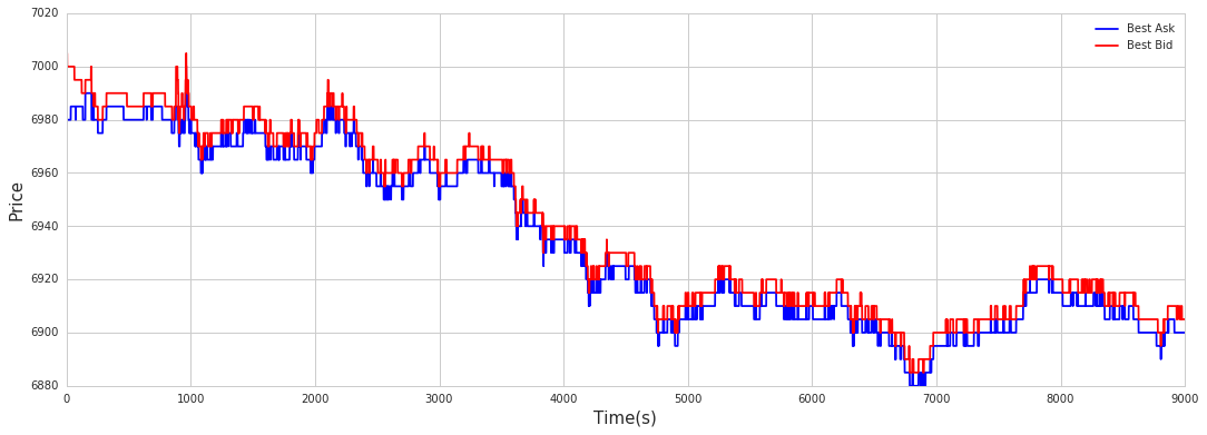
This block is setting up a simple time-series visualization of the best bid and best ask prices so you can visually inspect intraday microstructure behavior for a particular slice of the 2014 dataset. First we choose a clean plotting style (whitegrid) and allocate a wide figure (18x6 inches) to make fine-grained price movements and small spreads readable — that’s important in quant trading because tiny spread changes or brief quote spikes can be actionable signals or evidence of data issues. The code then defines a small palette and plots two series from data_2014[1]: the column keyed by ‘66’ as the best ask and the column keyed by ‘67’ as the best bid. Displaying both on the same axes makes it easy to see the bid–ask spread, mid-price dynamics, quote crossings, and any latency or stale-quote artifacts; consistent color choices help you immediately distinguish the two series when scanning charts.
A legend is added so the series labels (“Best Ask” and “Best Bid”) are clear, and the axes are labeled with units (Time(s) on x, Price on y) to tie the chart back to the trading context — the x-axis here is the observation index interpreted as seconds, which matters because temporal resolution and alignment drive interpretation of order book dynamics. In practice this visual check supports several quant workflows: validating data integrity (e.g., detecting missing or stale quotes), exploring spread behavior for feature engineering (how often and by how much spread widens), and confirming that any downstream signals based on bid/ask relationships are operating on sensible inputs.
A couple of implementation notes that follow from the “why”: ensure data_2014[1] is properly time-aligned (timestamps converted to actual seconds if needed) before trusting temporal inferences; for very high-frequency streams you may need decimation or transparency to avoid overplotting; and often it’s useful to compute and plot the spread or mid-price alongside raw quotes to simplify quantitative analysis rather than relying solely on visual inspection.
One Day Accuracy
sns.set_style(”whitegrid”)
plt.figure(figsize = (18,6))
color = []
for key in pip.keys:
    plot(np.array(pip.acc_day[key])[0],’-o’,label = key,lw = 1,markersize = 3)
    plt.legend(loc=0)
plt.ylim(-0.5,1.5)
plt.legend(loc=0)
plt.xlabel(’Rolling Window Numbers’,size = 15)
plt.ylabel(’Accuracy’,size = 15)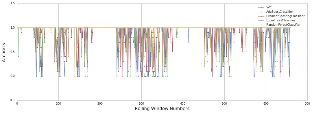
This block’s purpose is to produce a comparative time-series chart of model/strategy accuracy across a sequence of rolling windows so you can visually assess stability and relative performance for quant trading decisions (e.g., whether a model is drifting, when to retrain, or which signal to allocate capital to). It begins by setting a clean grid style and a wide figure so the horizontal axis (rolling windows) is easy to read — a wide aspect is useful for time/sequence plots where you want trend detail rather than a cramped view. The plotting loop then iterates the set of “keys” (each key represents a model, strategy, or asset) and for each one it pulls the stored accuracy series from pip.acc_day keyed by that identifier, coerces it into a NumPy array and selects the first row. That 1-D sequence is drawn as a connected line with small circular markers so you can inspect both pointwise accuracy and the trend across windows; the line width is kept thin to avoid overwhelming the chart when multiple lines overlap, and markersize is small to keep the plot tidy.
Several decisions in the code reflect practical visualization and analysis concerns. The y-axis limits are fixed between −0.5 and 1.5 to provide consistent scale across plots and to center a typical accuracy range [0,1] with a bit of padding so points don’t sit on the border; consistent scaling makes it easier to compare stability and volatility of accuracy between keys. The legend is requested (loc=0 means “best” placement) so each line is identifiable: this supports quick interpretation when choosing models to deploy or retire. Using a grid style improves the ability to read values and identify change points that might indicate regime shifts or model degradation — important signals in quant trading where performance can vary by market regime.
A few implementation notes and suggested cleanups (why they matter): the code takes the first row via [0] which implies the stored accuracies are nested (e.g., a 2D container containing a single row); that extraction is brittle if the data shape changes, so converting to a true 1-D sequence with ravel/flatten or validating shape first is safer and makes the visualization robust to data structure variations. The legend call inside the loop is redundant and expensive; calling it once after the loop is cleaner and avoids repeated layout calculations. The unused color list and use of a top-level plot function (instead of the explicit plotting namespace) are minor issues that can confuse readability — using the plotting module explicitly and removing unused variables clarifies intent. Finally, ensure you’re iterating the actual iterable of keys (e.g., keys() versus a keys attribute) so the loop behaves correctly.
In the context of model lifecycle and risk decisions for quant trading, this plot is a diagnostic tool: it reveals which models hold stable accuracy across rolling windows (candidates for production), which spike or collapse (candidates for further investigation), and where to trigger retraining or reduce allocation. Small implementation cleanups will make the chart more reliable and maintainable so it continues to provide good operational signals.
Cross-validation
sns.set_style(”whitegrid”)
plt.figure(figsize = (18,6))
color_ = [’r’,’orange’,’y’,’g’,’b’]
for index,key in enumerate(pip.keys):
    plot(np.array(pip.cv_acc_day[key])[0],’-o’,label = key,color = color_[index],lw = 1,markersize = 3)
#plot(best_cv_score,’-v’,label = ‘Best cv 5 folds score’,color = ‘violet’,lw = 1,markersize = 6)
plt.legend(loc=0)
plt.xlabel(’Rolling Window Numbers’,size = 15)
plt.ylabel(’CV Mean Accuracy’,size = 15)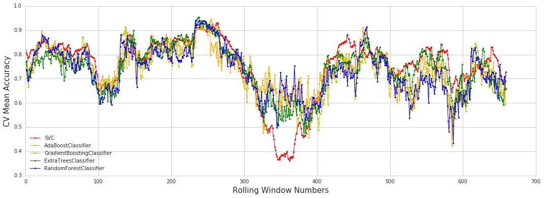
This block builds a diagnostic line-plot that compares cross‑validation (CV) mean accuracy across a series of rolling-window retrains for multiple models/instruments. It first switches to a light grid aesthetic and creates a wide plotting canvas so multiple short series can be compared horizontally; that layout choice favors readability when you are inspecting performance variation across many window lengths. The core data source is pip.cv_acc_day indexed by pip.keys: each key represents a model, asset, or strategy variant, and pip.cv_acc_day[key] contains the per-window CV accuracy results. Converting that object to a NumPy array and taking [0] extracts the primary summary vector (the mean CV score for each rolling window) that we want to visualize — this normalization step ensures the plotting routine receives a simple 1‑D numeric series regardless of how the results were originally nested.
Inside the loop, each series is plotted as a thin line with small circular markers and a distinct color; the line makes trends over window length easy to see, while the markers make individual window values discernible. Assigning a label to each series and later calling legend(loc=0) places a concise, automatically positioned key on the plot so you can immediately map curves back to specific models/strategies. The commented-out plot call shows an alternative to overlay a single “best CV across k‑folds” summary in a contrasting style, which can be used to highlight the single best configuration against the per‑model traces.
From a quant trading perspective, this visualization is purposeful: it surfaces how stable each model’s cross‑validated accuracy is as you change the rolling retrain window, helping you detect models that overfit transient patterns (large swings) versus those that generalize (flat, stable lines). The stylistic choices (grid, modest line width, markers, distinct colors) are practical decisions to minimize visual clutter while preserving the ability to compare subtle performance differences.
Best Model
sns.set_style(”whitegrid”)
plt.figure(figsize = (18,6))
plot(best_cv_score,’-o’,label = ‘Best cv 5 folds score’,color = ‘violet’,lw = 1,markersize = 5)
plt.legend(loc=0)
plt.xlabel(’Rolling Window Numbers’,size = 15)
plt.ylabel(’CV Mean Accuracy’,size = 15)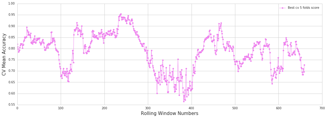
This block is purely about presenting the results of cross‑validation across a set of rolling‑window configurations so you can visually decide which lookback length or data window is most robust for your trading model. First, the plotting style is set to a clean white grid to make small differences and alignment against the axes easy to read; for quant workflows where we compare many adjacent window sizes, a consistent grid helps spot trends and small inflections that matter for model selection. A figure with an explicitly large width is created so that each rolling‑window point has enough horizontal space; this prevents cramped labels and overlapping markers when you sweep many window sizes and makes the plot usable in reports or notebooks.
Next, the series best_cv_score is drawn as a connected line with circular markers (‘-o’), which tells the viewer both the trend across window numbers and the precise CV mean at each point. The connection emphasizes monotonic or systematic behavior across windows (e.g., steadily improving or degrading performance) while the markers let you zero in on exact scores for individual windows. The color, line width and marker size choices are simply aesthetic controls to ensure the data is visible but not visually noisy — thin line to show the trend, distinct marker color to highlight points. A legend is added with automatic placement so it won’t obscure the data; in practice this makes the plot self‑documenting when multiple series are present (e.g., comparing different models or hyperparameter sets).
Finally, the x and y labels map the visual elements back to the quant trading decision: the x‑axis indicates the rolling window index (the different lookback/window sizes you tested) and the y‑axis reports the 5‑fold CV mean accuracy used as the selection metric. The purpose of this visualization is to help you identify windows that deliver consistently good CV performance (not just a noisy spike), to detect sensitivity to window choice, and to avoid chasing single high points that may be artefacts of particular folds. In practice you’ll often complement this plot with measures of fold variability (error bars or shaded std) and other metrics (precision/recall, Sharpe estimates on out‑of‑sample returns) before committing to a window choice for live trading.
sns.set_style(”whitegrid”)
plt.figure(figsize = (18,6))
color_ = [’r’,’orange’,’y’,’g’,’b’]
for index,key in enumerate(pip.keys):
    plot(np.array(pip.cv_acc_day[key])[0][0:250],’-o’,label = key,color = color_[index],lw = 1,markersize = 5)
#plot(best_cv_score,’-v’,label = ‘Best cv 5 folds score’,color = ‘violet’,lw = 1,markersize = 6)
plt.legend(loc=0)
plt.xlabel(’Rolling Window Numbers’,size = 15)
plt.ylabel(’CV Mean Accuracy’,size = 15)
plt.ylim(0.55,1)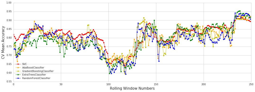
This block builds a visual diagnosis of model stability by plotting the cross-validated mean accuracies for several pipelines across a sequence of rolling windows — a common way in quant trading to check how model performance changes through time as you re-train or re-evaluate on successive windows. It starts by choosing a clean, grid-backed plotting style and a wide figure so many consecutive windows can be displayed without crowding; these choices improve readability when you want to inspect temporal patterns and small differences between models.
Inside the loop, each pipeline identified by pip.keys is drawn as a separate line. The code converts pip.cv_acc_day[key] to a NumPy array and then indexes into the first row before taking the first 250 entries. Practically, that [0] is selecting the sequence of mean CV accuracies (the stored structure is nested, so the explicit conversion and first-row selection make sure we pass a 1‑D numeric series to the plotter), and the [0:250] slice deliberately limits the plot to the first 250 rolling windows to keep the chart focused and uncluttered. Each series is drawn with a distinct color, small marker and thin line so you can see the discrete per-window points and the overall trend without overwhelming the figure; labels are attached so the legend maps lines back to pipeline names.
After the lines are drawn the legend is shown, axis labels are added to communicate that the x-axis indexes rolling-window positions and the y-axis reports CV mean accuracy, and the y-limits are constrained to [0.55, 1]. That y-range is a deliberate choice to zoom in on the useful band of predictive performance seen in trading models — it makes small but economically relevant differences visually apparent — but it does mean any accuracy below 0.55 will be clipped and not visible. The commented-out plot indicates a previously considered overlay of a “best 5-fold CV” baseline; re-enabling it would let you compare each rolling-window mean against a single global benchmark.
sns.set_style(”whitegrid”)
plt.figure(figsize = (18,6))
plot(best_cv_score[0:250],’-o’,label = ‘Best cv 5 folds score’,color = ‘violet’,lw = 1,markersize = 5)
plt.legend(loc=0)
plt.xlabel(’Rolling Window Numbers’,size = 15)
plt.ylabel(’CV Mean Accuracy’,size = 15)
plt.ylim(0.55,1)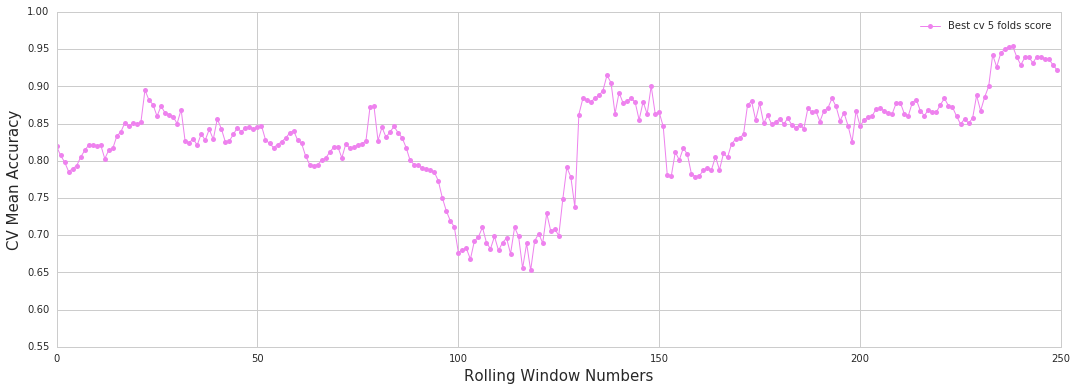
This block prepares a focused diagnostic plot that tracks model performance across a sequence of rolling-training windows — in our case the first 250 windows — so we can visually inspect temporal stability of the 5-fold cross-validation results. We set a clean whitegrid style and an 18x6 aspect ratio to make a long time-series easy to read: the horizontal stretch favors many sequential windows while the grid gives subtle visual anchors for small changes. Choosing a wide figure is intentional for quant workflows because we often need to compare many adjacent rolling windows without compressing individual fluctuations into noise.
We then draw a connected line with markers for each window’s best CV mean accuracy (best_cv_score[0:250]) so two things are achieved simultaneously: the line highlights trend and direction across windows, while the point markers expose per-window volatility and any outliers. Using a distinct color and a modest line width/marker size keeps the plot legible when many points are present; the label clarifies that these values are the mean accuracy from a 5-fold cross-validation, i.e., the estimator’s expected generalization performance within each rolling sample. The legend is placed automatically (loc=0) to avoid overlapping the data, which is useful when inspecting many different performance plots side-by-side.
Axis labels explicitly connect the visualization back to the quant-trading workflow: the x-axis enumerates rolling windows (sequential training/testing periods), and the y-axis is CV mean accuracy, the proxy for short-term model efficacy. We clamp the y-limits to the [0.55, 1.0] range to zoom into the practically relevant band for our models — this prevents the visual impression from being dominated by an uninformative global range and makes smaller but meaningful degradations or improvements visible. Choosing that lower bound (0.55) reflects a judgment that anything below it is effectively non-informative for our strategy and should be scrutinized separately.
Operationally, this plot is meant to answer questions critical to production quant systems: Is performance stable across market regimes, or do we see systematic decay or spikes that suggest overfitting, data leakage, or regime change? Persistent downward trends or sudden drops indicate model drift or feature-relevance shifts and should trigger retraining, feature re-examination, or alternative model selection. Conversely, near-perfect, flat performance across many windows can be a red flag for look-ahead bias or leakage. In short, these stylistic and range choices are deliberate to make model stability and anomalous windows immediately apparent to a quant practitioner.
Profit and Loss
# compute cum_profit and Best_cv_score
dict_ = {}
dict_[’cum_profit’] = []
dict_[’Best_cv_score’] = []

for day in range(0,1,1):
    cum_profit_label = []
    cum_profit = []
    best_cv_score = []
    spread = 0.2 * data_2014[day][’65’][1800:][9::10].values
    loss = 0.2*(data_2014[0][’67’][1800:9000-600][9::10].values - data_2014[day][’67’][1800+600:9000][9::10].values)
    for j in range(0,len(pip.cv_acc_day.values()[0][day]),1):
        max_al = {}
        for i in range(0,len(pip.keys),1):
            max_al[pip.keys[i]] = np.array(pip.cv_acc_day[pip.keys[i]])[day][j]
        # select best algorithm in cv = 5
        top_cv_acc = sorted(max_al.items(),key = lambda x : x[1], reverse = True)[0:1][0]
        best_cv_score.append(top_cv_acc[1])
        submission = pip.predict_values_day[top_cv_acc[0]][day][j][-1]
        true_value = pip.true_values_day[top_cv_acc[0]][day][j][-1]

        if submission == true_value:
            if submission == 1:
                cum_profit_label.append(1)
                cum_profit.append(spread[j])
            elif submission == 0:
                cum_profit_label.append(0)
                cum_profit.append(0)
        elif submission != true_value:
            if submission == 1:
                cum_profit_label.append(-1)
                cum_profit.append(loss[j])
            elif submission == 0:
                cum_profit_label.append(0)
                cum_profit.append(0)

    dict_[’cum_profit’].append(cum_profit)
    dict_[’Best_cv_score’].append(best_cv_score)
This block is evaluating trade-level profit outcomes by selecting, for each prediction opportunity, the single model with the highest cross‑validation accuracy and then applying that model’s final prediction to compute realized P&L. At the top level we build two output lists — cum_profit (the monetary P&L per trade) and Best_cv_score (the CV accuracy of the model chosen for that trade) — and append per‑day lists into dict_. The outer loop is written to iterate days, although with range(0,1,1) it effectively runs for a single day; the same logic generalizes to multiple days.
For the chosen day we precompute two series used to turn a correct or incorrect directional call into money: spread and loss. spread is a scaled slice of a price series (data_2014[day][‘65’]), subsampled by [9::10] and multiplied by 0.2; it represents the reward when a long trade is placed and the model is correct. loss is computed as 0.2 times the difference between two aligned slices of another price series (‘67’) shifted by 600 samples (data_2014[0][‘67’][1800:9000–600] minus data_2014[day][‘67’][1800+600:9000]); that subtraction produces the adverse move we would realize if a long trade is wrong after the intended holding period. In other words, spread is the profit for a correct long, and loss is the realized price move against us for an incorrect long — the 600‑step offset encodes the assumed trade duration.
The inner loop iterates over each prediction instance j for that day. For each j we build a mapping max_al of algorithm → CV accuracy by extracting the CV accuracy for that specific day and instance from pip.cv_acc_day for every algorithm in pip.keys. We then choose the single top algorithm by sorting these accuracies and taking the highest entry; its accuracy is appended to best_cv_score so we can later analyze the distribution of chosen CV scores. Using the chosen algorithm’s name we pull the final predicted label (submission) and the actual label (true_value) for that day/instance; those are the values used to decide the trade outcome.
The trading logic imputes that a prediction value of 1 means “enter a long trade” and 0 means “do not trade” (or equivalently, no exposure). If submission == true_value and submission == 1 we record a successful long: cum_profit_label gets +1 and cum_profit gets spread[j]. If submission == true_value and submission == 0 we record a correct “no trade” with zero P&L. If submission != true_value and submission == 1 we record a failed long (label -1) and the negative P&L equal to loss[j]. If submission != true_value and submission == 0 we again record zero P&L — predicting no trade never generates P&L in this logic, whether correct or not. At the end of the per‑day loop the code appends the per‑instance cum_profit and Best_cv_score lists to dict_ for downstream aggregation or analysis.
Why this design: by selecting the algorithm with the best CV accuracy for each instance, the code tries to exploit model heterogeneity at the finest granularity, effectively performing per‑trade model selection to maximize the chance of a correct directional call. The separation of spread and loss (and the 600‑step offset) enforces a realized P&L calculation tied to a fixed holding period and scaled to the business unit (0.2). The cum_profit_label vector provides a compact view of trade correctness (+1, 0, -1), while cum_profit gives the economic consequence, so you can compute aggregate metrics (total P&L, hit rate weighted by P&L, drawdown, etc.).
sns.set_style(”whitegrid”)
plt.figure(figsize = (20,8))
plt.subplot(211)
plot(cum_profit,’-o’,label = ‘Profit & Loss’,lw = 1,markersize = 3)
plt.ylabel(’Tick’,size = 15)
plt.legend(loc=0)
plt.ylim(-7.5,2.5)
plt.subplot(212)
plot(cumsum(cum_profit),’-o’,label = ‘Cum Profit’,lw = 1,markersize = 2)
plt.legend(loc=0)
plt.xlabel(’Rolling Window Numbers’,size = 15)
plt.ylabel(’Profit’,size = 15)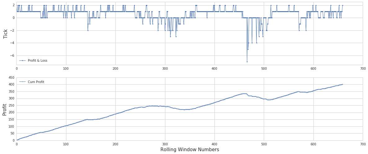
This block creates a two-panel diagnostic plot intended to help evaluate short‑term P&L behavior and its accumulation over a sequence of rolling windows — a common visualization when validating a quant strategy across parameter windows or time slices.
First, the code sets a clean grid style and a wide figure so lots of points and subtle variations are readable. The top subplot (211) plots the per‑window P&L series (named cum_profit here) as a connected line with small markers. The intention is to show the granular, tick‑level or window‑level fluctuations — individual wins and losses — so you can inspect volatility, outliers, and whether the per‑window returns are centered around a particular level. The y‑axis is labeled “Tick” which implies these values are expressed in ticks per window; the explicit y‑limits (-7.5 to 2.5) are chosen to fix the visual scale so that small variations aren’t lost to autoscaling and so multiple runs can be compared consistently. A compact line width and small markers keep the plot legible when there are many points.
The bottom subplot (212) transforms that same sequence into a running total via cumulative sum, plotting the aggregated P&L across the rolling windows. This cumulative view answers the “so what” question: regardless of noisy per‑window behavior, does the strategy net positive performance over the sequence, or does it drift into sustained drawdown? Plotting cumulative profit makes trends, persistent biases, and the timing of drawdowns immediately visible; the x‑axis labelled “Rolling Window Numbers” makes clear the independent variable is the window index rather than calendar time. The legend placement is left to the plotting backend (loc=0), and slightly different marker sizing and line weight are cosmetic choices to balance point visibility against line clutter.
Together, the two panels let you diagnose both local behavior (is each window profitable, how noisy is it, are there spikes) and global behavior (does noise average out to a positive drift, are there regime shifts or large cumulative drawdowns). These insights inform next steps in a quant workflow — for example, adjusting signal construction, changing stop/size rules, normalizing by volatility, or re‑examining window selection — because they reveal whether issues are transient, systematic, or scale‑dependent.
