Quantitative Finance with Python: Arbitrage & Asset Pricing

A step-by-step guide to writing trading algorithms and modeling stock expected returns using real-world market data.

Download the entire source code using the button at the end of this article!

Welcome to the intersection of quantitative finance and data science. If you have ever wondered how trading algorithms actually work under the hood, this article bridges the gap between financial theory and practical Python code. We will explore two foundational, yet highly distinct, market strategies: the rapid-fire world of Arbitrage Trading and the classic valuation principles of the Capital Asset Pricing Model (CAPM).

First, you will dive into a Pure Arbitrage Trading Algorithm. Using historical Bitcoin pricing data as a testing ground, you will learn how to write Python code using pandas and numpy to detect short-lived price imbalances across different exchanges. You won’t just look at theoretical spreads; you will read through line-by-line implementations that account for real-world constraints like transaction fees to generate mathematically sound execute/no-execute trading signals.

Next, the article shifts to traditional equities to break down the Capital Asset Pricing Model (CAPM). You will find a comprehensive guide on fetching historical stock and market data (such as the S&P 500 and 10-year Treasury yields), calculating periodic returns, and running Ordinary Least Squares (OLS) regressions using statsmodels. By the end, you will understand exactly how to calculate a stock’s Beta and plug it into the CAPM equation to forecast expected returns, complete with a thorough statistical breakdown of the results.

Arbitrage Trading Algorithm

Pure Arbitrage (Pure Arb) -> Cross Exchange Arbitrage

- Depends on ultra-low latency and the ability to detect short-lived price imbalances across venues.

- Executes offsetting trades at the same time on different markets — buying on the cheaper venue and selling on the pricier one — to capture the spread.

The opportunity set is large in theory, but practical profitability requires the fastest execution and careful accounting for costs; for example, the notebook aligns Gemini and Reuters prices, computes the absolute spread, estimates fees (0.2% of the two prices combined), and only treats opportunities as executable when the spread exceeds those estimated fees.

import pandas as pd
import numpy as np

The two import statements load two core Python libraries used for data analysis and numerical work. Importing a module makes its functions, classes, and constants available in the current program so you can call them by name. Here the modules are given short, conventional aliases: pandas as pd and numpy as np, which just saves typing and follows common practice in the data-science community.

Pandas (pd) provides high-level structures like DataFrame and Series and lots of tools for reading, reshaping, indexing, grouping, and summarizing tabular data. You’ll typically call things like pd.read_csv or pd.DataFrame, and use methods for aligning, merging, and aggregating time series or tables.

NumPy (np) supplies the ndarray (n-dimensional array) and fast, vectorized numerical operations, broadcasting rules, random number generation, and many mathematical functions. Operations done with np arrays are much faster than equivalent pure-Python loops for large numeric datasets, and many pandas operations are implemented on top of NumPy arrays.

- pd.DataFrame, pd.read_excel, pd.concat, etc., for table manipulation

- np.array, np.where, np.unique, arithmetic and vectorized math for numerical work

If either library isn’t installed in the environment, these import lines would raise an ImportError; otherwise they silently succeed.

gemini = pd.read_excel(’BTCPrices.xlsx’,sheet_name = ‘Gemini’, na_values=None) # You would replace these datasets with 
# live streamed data.
reuters = pd.read_excel(’BTCPrices.xlsx’, sheet_name = ‘Reuters’) # Note that you can’t actually trade Crypto on Eikon Reuters.
# This is just pricing history data. (and an example.)

These two lines load two sheets from an Excel file into pandas DataFrame objects and assign them to the names gemini and reuters.

pd.read_excel(‘BTCPrices.xlsx’, sheet_name=’Gemini’, na_values=None) tells pandas to open the file BTCPrices.xlsx, read the sheet named “Gemini” and return its contents as a DataFrame. The na_values=None argument says “don’t add any extra strings to pandas’ list of things to treat as missing” (it’s effectively the default behavior). After this line runs, gemini refers to an in-memory table containing whatever columns and rows were on the Gemini sheet.

pd.read_excel(‘BTCPrices.xlsx’, sheet_name=’Reuters’) does the same for the sheet named “Reuters”, using pandas’ default missing-value handling because na_values wasn’t specified there. The returned DataFrame is stored in reuters.

A couple of practical notes embedded in the comments: the code expects the Excel file to be accessible from the working directory (otherwise you’ll get a FileNotFoundError), and the author is indicating that in a real trading system you’d typically replace static Excel input with live data streams. The comment about Reuters is just context: the sheet here is historical pricing data used for the example, not a live tradable crypto feed. There’s no printed output from these lines unless you explicitly display the DataFrames; the effect is that two DataFrame variables are created and ready for further processing.

Exchanges with public APIs suitable for arbitrage scanning

These platforms provide REST/WebSocket endpoints you can query for price and order-book data to build aligned time series (similar to the Gemini “Open” series used in the notebook):

- Binance API

- Bittrex API

- Poloniex API

- Coinbase API

- Kraken API

- Bitfinex API

- Bitstamp API

- HitBTC API

- Gemini API

- KuCoin API

gemini = gemini.set_index(”Date (EST)”)
gemini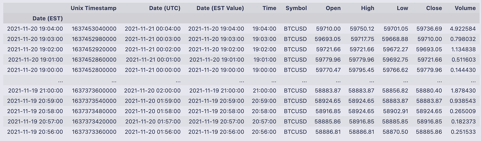

That line replaces the DataFrame’s default row index with the values from the “Date (EST)” column and stores the result back into the variable gemini. set_index returns a new DataFrame (it doesn’t modify in place unless you ask it to), so assigning it back to gemini makes the timestamp column become the row labels for every subsequent operation.

The printed table shows what that looks like: the leftmost field is now the index labeled Date (EST) and contains timestamp-like entries such as 2021–11–20 19:04:00, 2021–11–20 19:03:00, etc. To the right of that index you can see the DataFrame’s columns for each timestamp — things like Unix Timestamp, Date (UTC), Date (EST Value), Time, Symbol, Open, High, Low, Close and Volume. For example, the first displayed row (index 2021–11–20 19:04:00) has Open = 59710.00, High = 59750.12, Low = 59701.05, Close = 59736.69, and Volume = 4.922584. The output summary at the bottom tells you there are 1,329 rows and 10 columns after this change.

Using the timestamp column as the index makes the rows addressable by time (you can visually scan by datetime on the left), which is convenient whenever you want to slice, align or plot the data along the time axis.

reuters = reuters.set_index(”Time”)
reuters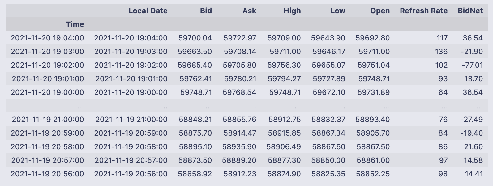

That single line replaces the DataFrame’s current row numbering with the values from the “Time” column and assigns that new indexed version back to the name reuters. set_index(“Time”) returns a new DataFrame whose rows are labeled by the entries that used to live in the “Time” column; because the result is assigned back into reuters, the variable now holds that indexed DataFrame (there’s no separate temporary left behind).

- Local Date

- Bid

- Ask

- High

- Low

- Open

- Refresh Rate

- BidNet

You’ll also notice the index values (the times) are repeated in the Local Date column in the sample rows — that just means the original sheet had both a Time column and a Local Date column, and only the Time column was promoted to the index here. The printed snapshot shows the first few and last few rows (top and bottom of the DataFrame) with numeric Bid/Ask/Open/etc. values, and the index on the left makes it easy to refer to or slice rows by those timestamps going forward.

import matplotlib.pyplot as plt
from matplotlib.pyplot import figure

The first line brings in Matplotlib’s pyplot module and gives it the common short name plt. Pyplot is a convenient, stateful plotting interface: it provides functions like plot, scatter, hist, xlabel, ylabel, title, legend and show, and it manages the “current” figure and axes so you can build plots with a sequence of simple calls (for example, plt.plot(…); plt.xlabel(…); plt.show()).

The second line imports the figure function itself directly into the local namespace. figure(…) is the constructor that creates a new Figure object (you can pass options like figsize and dpi). Because you imported it directly, you can call figure(…) without the plt. prefix; alternatively you can call plt.figure(…). Both refer to the same function, so this is essentially a convenience / redundancy: it saves you from typing plt. when you only need to create a Figure.

Neither line produces any visual output by itself — they just make plotting functions available. In a script you generally need plt.show() to force display; in many interactive notebook environments the backend will render plots automatically after plotting commands. One minor caution: doing from matplotlib.pyplot import figure brings that name into your global names, so if you later assign a variable called figure you’ll shadow the function. Otherwise, importing both plt and figure is harmless and common when you want the full plt API but also like calling figure(…) directly.

figure(figsize=(8, 4), dpi=200)
gem_BTC = gemini[’Open’]
reu_BTC = reuters[’Open’]
plt.plot(gem_BTC, label = “Gemini BTC”)
plt.plot(reu_BTC, label = “Reuters BTC”)
plt.title(’BTC Opening Prices’)
plt.legend()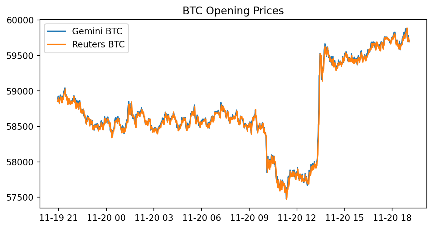

First the code allocates a plotting canvas with figure(figsize=(8, 4), dpi=200). That means matplotlib creates an 8 by 4 inch figure at 200 dots per inch, so the resulting image is 1600×800 pixels — a large, high-resolution plot.

Next two variables are created by pulling the “Open” column out of two existing pandas DataFrames: gem_BTC = gemini[‘Open’] and reu_BTC = reuters[‘Open’]. These are pandas Series of opening prices, and because they come from DataFrames with time-like indexes, plotting them will put those timestamps on the x-axis and the price values on the y-axis.

plt.plot(gem_BTC, label=”Gemini BTC”) and plt.plot(reu_BTC, label=”Reuters BTC”) draw the two price series on the same axes and attach the labels that are later used by the legend. plt.title(‘BTC Opening Prices’) sets the chart title, and plt.legend() draws the legend so you can tell which color corresponds to which source.

The displayed figure shows a blue line for Gemini and an orange line for Reuters that track each other very closely for the whole time span. The y-axis runs roughly from about 57,500 up to 60,000, and you can see a fairly abrupt upward jump partway through the timeline (around the middle-right of the plot) where both series rise together. For most of the chart the two lines almost overlap; small visible deviations are the moments when the two sources differ by a bit. The cell output also printed a matplotlib.legend.Legend object (that’s just the return value from plt.legend()) and the rendered figure is shown below it.

If you want to highlight the differences between the feeds more clearly, a next step would be to plot their difference (gem_BTC — reu_BTC) or to add transparency/markers so small gaps are easier to spot.

figure(figsize=(8, 4), dpi=400)
plt.plot(abs(gem_BTC - reu_BTC), label = “Spread |Gemini - Reuters|”)
plt.title(’Spread |Gemini - Reuters|’)
plt.legend()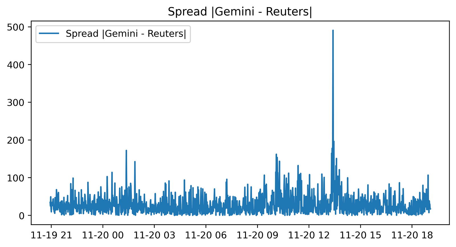

We start by making a new matplotlib figure with figure(figsize=(8, 4), dpi=400). That call sets the canvas size to 8 by 4 inches and a high resolution of 400 dots-per-inch, so the produced image is 3200×1600 pixels (8*400 by 4*400).

Next plt.plot(abs(gem_BTC — reu_BTC), label=”Spread |Gemini — Reuters|”) draws a single line: the absolute difference between the two Series gem_BTC and reu_BTC. Because those are pandas Series, the subtraction is done elementwise with alignment by their indexes, so each plotted point is the absolute spread at a given timestamp. The label you passed will be used in the legend. plt.title(…) puts the title “Spread |Gemini — Reuters|” above the plot, and plt.legend() shows the legend (the notebook prints the Legend object).

The displayed figure is a time series of that absolute spread. Most of the line sits at a relatively low level with continuous small fluctuations, there are short bursts of larger spreads in places, and one very large spike stands out well above the rest about two‑thirds of the way across the x‑axis. The x‑axis corresponds to the Series index (timestamps) and the y‑axis is the spread in the same price units as the original Series; numerical axis labels aren’t emphasized in this image but the shape and relative magnitude of the spread over time are clear. The printed output shown in the notebook is the Legend object and a description of the created Figure.

# Sum of the entire spread?
sum(abs(gem_BTC - reu_BTC))# In a PERFECT environment. This does not include fees. If via BTC,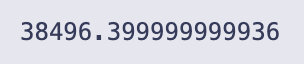

You’re taking the per-row difference between the two price series, turning those differences into absolute values, and then adding all of them up to get a single scalar.

Concretely:

- gem_BTC — reu_BTC computes the elementwise difference between the two pandas Series (pandas lines up values by index labels when you do this).

- abs(…) takes the absolute value of each of those differences so every entry is a non-negative spread.

- sum(…) adds up all those absolute spreads into one total number.

The printed result, 38496.399999999936, is that total. The long tail after the decimal is just floating-point representation; you can read it as roughly 38496.4 in whatever units your series use (e.g., dollars if these are USD BTC prices). The inline comment is correct: this is a perfect-environment aggregate of raw spreads and does not account for trading fees, slippage, or any transaction constraints.

# Buy Low in one exchange and sell high in the other exchange.
# Let’s combine the necessary columns together.
# 0.2% average between maker and taker.
comb_df = pd.concat([gem_BTC,
                     reu_BTC,
                     abs(gem_BTC - reu_BTC),
                     0.002 * (gem_BTC + reu_BTC)], axis = 1) 
comb_df.columns = [”Gemini_Open”, “Reuters_Open”, “Absolute_Difference”, “Total_Tax”]
comb_df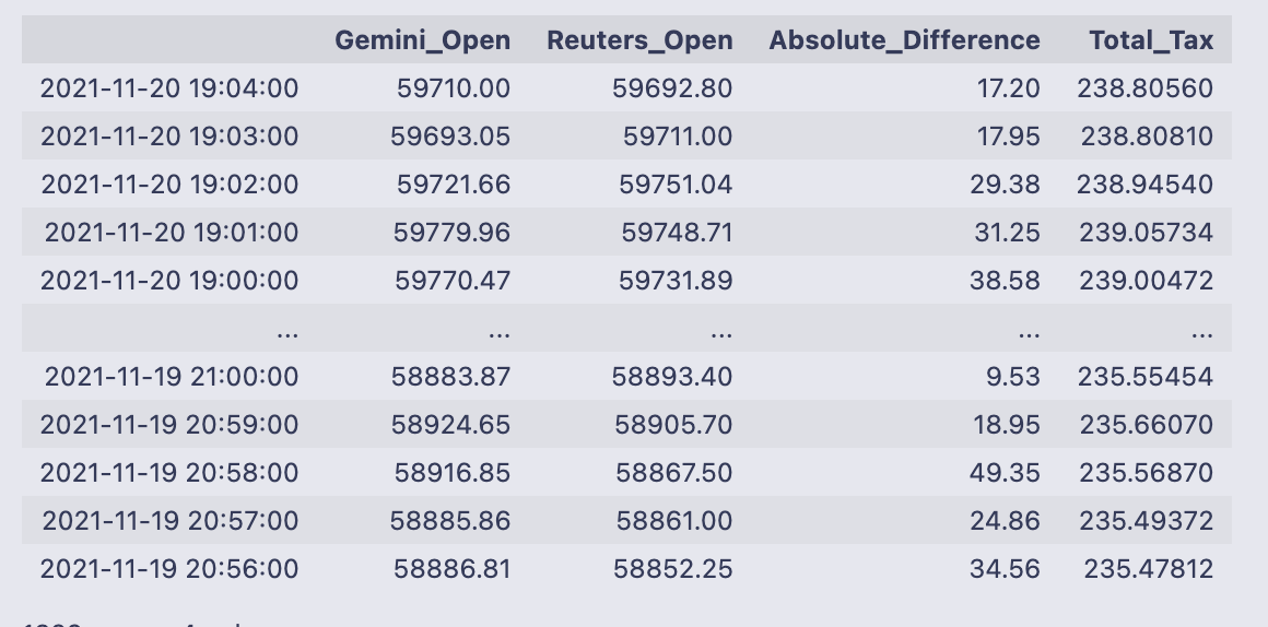

You take two price series and build a single table that puts the raw prices next to two simple calculations that are useful for deciding whether an arbitrage is worth executing.

First you call pd.concat with four column inputs and axis=1, which stacks them side-by-side as columns (pandas aligns each input by its index, so values line up by timestamp). The four columns are:

- gem_BTC (Gemini opening price),

- reu_BTC (Reuters opening price),

- abs(gem_BTC — reu_BTC) (the absolute spread between the two prices),

- 0.002 * (gem_BTC + reu_BTC) (an estimated total fee equal to 0.2% of the combined price).

After concatenation you rename the columns to [“Gemini_Open”, “Reuters_Open”, “Absolute_Difference”, “Total_Tax”] so the table is easier to read.

The printed DataFrame shows timestamped rows (the index is datetimes) with those four columns. Looking at the sample rows, the spreads (Absolute_Difference) are on the order of tens of dollars (e.g., 17.20, 31.25, 49.35) while the Total_Tax values are about 238 in these rows — that number comes from 0.002 * (Gemini_Open + Reuters_Open). For example, 0.002 * (59710.00 + 59692.80) = 238.8056, which matches the Total_Tax shown. Because the fee estimate is much larger than the spread in these examples, a naive glance suggests most individual spreads here would not cover the fee; the DataFrame makes it easy to check that across all timestamps.

Finally, pandas reports the table shape at the bottom: 1329 rows × 4 columns, confirming how many aligned timestamps ended up in this combined view.

# Check out which accounts in the corresponding exchanges need to be bought or sold.
v = pd.DataFrame(np.where(comb_df[”Gemini_Open”] > comb_df[”Reuters_Open”], 0,1))
v.index = comb_df.index
v.columns = [”BuyGemSellReuOrder”]
comb_df = pd.concat([comb_df, v], axis= 1)
comb_df # Exchange Signal = 0, Sell Gemini; Buy Reuters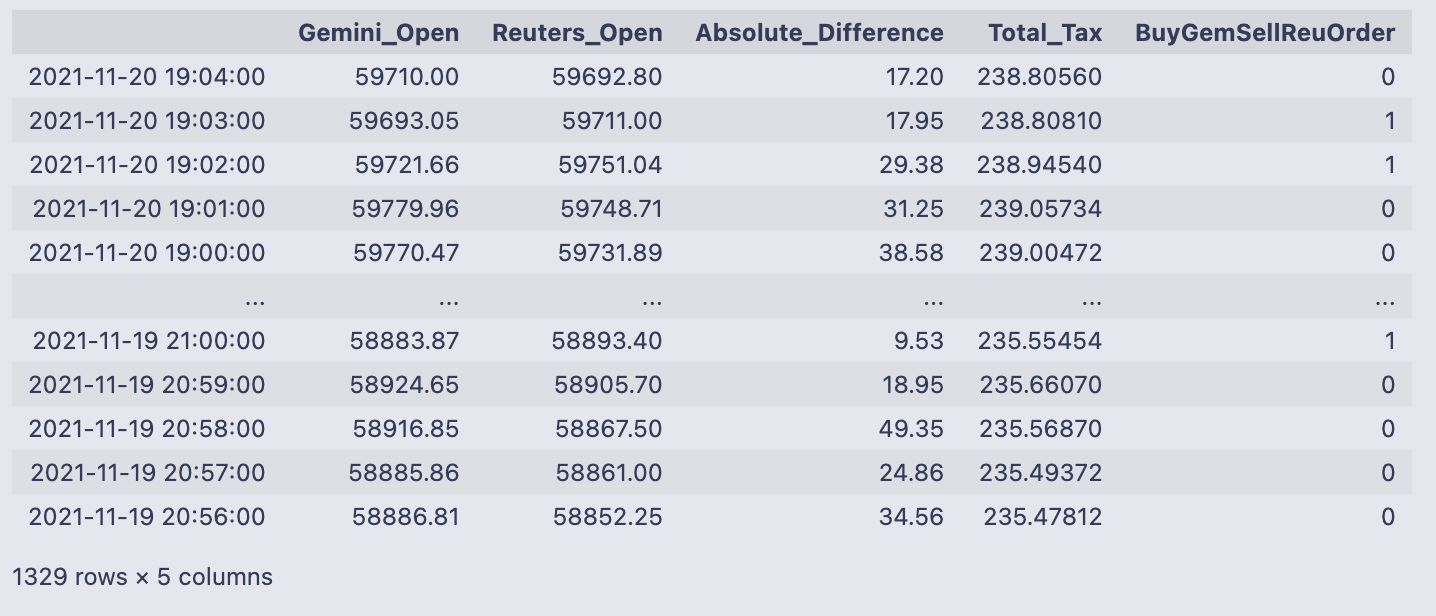

We build a simple buy/sell signal column and attach it to comb_df. np.where(comb_df[“Gemini_Open”] > comb_df[“Reuters_Open”], 0, 1) produces a numpy array of 0s and 1s: it writes 0 when the Gemini price is greater than the Reuters price, and 1 otherwise. Wrapping that array with pd.DataFrame gives us v, a one-column DataFrame with those integer signals.

- v.index = comb_df.index sets v’s index to be the same timestamps as comb_df so rows line up.

- v.columns = [“BuyGemSellReuOrder”] gives the new column a descriptive name.

pd.concat([comb_df, v], axis=1) then appends that single column to comb_df as a new column. The final comb_df is shown directly, so you can see the original columns (Gemini_Open, Reuters_Open, Absolute_Difference, Total_Tax) plus the new BuyGemSellReuOrder column of 0/1 signals.

Looking at the printed output ties the logic to real rows: the first line, timestamp 2021–11–20 19:04:00, has Gemini_Open 59710.00 and Reuters_Open 59692.80, so Gemini > Reuters and the signal is 0. The next row has Gemini_Open 59693.05 < Reuters_Open 59711.00, so the signal is 1. The table footer tells you there are 1,329 rows and 5 columns after adding the new signal column.

The intended interpretation (as noted in the inline comment) is: a 0 means “sell on Gemini and buy on Reuters” (because Gemini’s price is higher), while a 1 means the opposite direction. One small behavioral detail to notice: the test uses >, not >=, so exact price equality will be classified as 1 (the “otherwise” branch).

# Execute Trade for profit?
# Check out which accounts in the corresponding exchanges need to be bought or sold.
order66 = pd.DataFrame(np.where(comb_df[”Absolute_Difference”] > comb_df[”Total_Tax”], 0,1))
order66.index = comb_df.index
order66.columns = [”Execute”]
comb_df = pd.concat([comb_df, order66], axis= 1)
comb_df # Exchange Signal = 0, Sell Gemini; Buy Reuters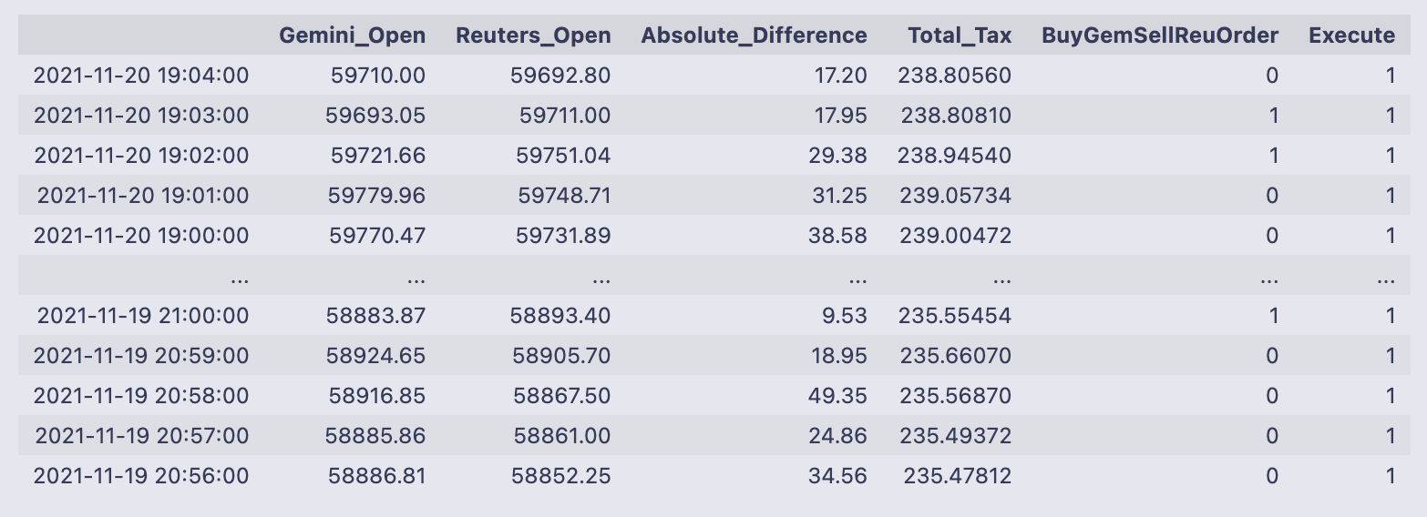

The code is creating a simple execute/no-execute signal and appending it to the existing table (comb_df). Concretely, np.where(comb_df[“Absolute_Difference”] > comb_df[“Total_Tax”], 0, 1) evaluates whether the absolute spread between the two prices is greater than the estimated total fee. If the spread is larger than the fee the expression yields 0, otherwise it yields 1. That array of zeros and ones is wrapped in a DataFrame called order66, its index is set to match comb_df.index so the rows line up, and the single column is named “Execute”. Finally the new DataFrame is concatenated onto comb_df along columns, so every row in comb_df now has an Execute flag.

- np.where returns a NumPy array of 0/1 values; converting to a DataFrame lets us set the index and a column name before concatenation.

- order66.index = comb_df.index ensures rows line up correctly; pd.concat(axis=1) just appends the column rather than inserting it by position.

- The code uses 0 to indicate a profitable/executable opportunity (spread > fee) and 1 to indicate don’t execute — that choice of coding (0 = execute, 1 = skip) is the convention used here.

The printed DataFrame confirms the new column appears beside the existing columns. For example, the top row shows Absolute_Difference = 17.20 and Total_Tax = 238.80560, so Execute is 1 (do not execute) because the fee estimate dwarfs the spread. The sample output shows mostly Execute = 1 in these rows, and the full table size is reported as 1329 rows × 6 columns, meaning every timestamp now carries the two prices, the spread, the fee estimate, the prior buy/sell direction column (BuyGemSellReuOrder), and this new Execute flag. When Execute equals 0, you know the row is flagged as potentially profitable; combined with the BuyGemSellReuOrder column (0/1 indicating which side to buy/sell) you have both the decision to act and the direction to act.

np.unique(comb_df[”Execute”], return_counts = True) #LOL!

You’re calling numpy’s unique function on the “Execute” column of comb_df and asking it to also return counts for each unique value. np.unique returns a tuple: the first element is a sorted array of the distinct values found, and the second element is an array of how many times each of those values occurs (aligned by position).

- array([0, 1]) — the distinct values present in the column (0 and 1).

- array([ 1, 1328], dtype=int64) — the counts for those values: the value 0 appears once, and the value 1 appears 1328 times.

So the “Execute” column is almost entirely 1s with a single 0. The little #LOL! comment suggests the author was amused or surprised by that imbalance.

# Let’s get a tally on all the orders that would’ve been executed.
orders_fulfilled = comb_df.loc[comb_df[”Execute”] == 0]
orders_fulfilled

The line orders_fulfilled = comb_df.loc[comb_df[“Execute”] == 0] builds a filtered view of comb_df by using a boolean mask: comb_df[“Execute”] == 0 produces True/False for every row, and .loc[…] returns only the rows where that condition is True. The next line (just the variable name) prints that filtered DataFrame so you can inspect the rows that matched.

The printed table shows a single row (indexed by the timestamp 2021–11–20 13:24:00) with these columns and values:

- Gemini_Open: 59216.09

- Reuters_Open: 58725.23

- Absolute_Difference: 490.86

- Total_Tax: 235.88264

- BuyGemSellReuOrder: 0

- Execute: 0

So what happened here: the code extracted all rows where the Execute flag equals 0 and displayed them. Only one row met that condition in this dataset. Looking at the numbers in that row, the absolute difference between the two prices (490.86) is larger than the Total_Tax value (235.88264), which explains why this row was flagged as an executable opportunity and ended up in orders_fulfilled. The BuyGemSellReuOrder column is 0 for this timestamp, showing whatever direction/signal encoding was used for that column in the table.

total_profits = sum(orders_fulfilled[”Absolute_Difference”] - orders_fulfilled[”Total_Tax”])
total_profits # would’ve made aroun $255 in one day for only ONE coin on 2 exchanges (Remember that Reuters doesn’t trade crypto)

total_profits is created by taking the per-row difference between two columns in the orders_fulfilled DataFrame — “Absolute_Difference” minus “Total_Tax” — and then summing all those row-wise differences into one scalar. In code terms, orders_fulfilled[“Absolute_Difference”] — orders_fulfilled[“Total_Tax”] produces a Series where each entry is the net amount (spread minus estimated fee) for one fulfilled order, and sum(…) adds up that Series into a single total.

When you evaluate total_profits the notebook prints 254.9773599999933. That number is the aggregate of all those per-order net amounts; the inline comment in the code interprets it as “about $255” for the set of orders included in orders_fulfilled. The long tail of digits is just floating-point representation — if you want a currency-style number you would typically round it to two decimal places (for example, round(total_profits, 2) -> 254.98).

# Notice that I am not even including the volume. (Hence everything will be a multiple)
# Retrieving that specific row:
gemini[comb_df[”Gemini_Open”] == 59216.09] # 27.31 BTC!!! Probably explains that huge discrpency amongst the “exchanges”.

The two commented lines set the intent and then do a simple lookup: comb_df[“Gemini_Open”] == 59216.09 creates a boolean Series that is True where the Gemini open price equals 59216.09, and then gemini[…] uses that boolean Series to select the matching row(s) from the original gemini DataFrame. Pandas aligns the boolean Series to gemini by index labels, so you get the full original row(s) for any timestamps where the Gemini open was exactly 59216.09.

- Open: 59216.09 (the value we matched)

- High/Low/Close: nearby price information (59347.67 / 59029.89 / 59218.88)

- Volume: 27.313468

That volume is the reason for the in-line comment: a 27.31 BTC trade is large enough to move or reflect a very different price on a single exchange, so seeing that large volume at the time of the 59216.09 quote helps explain why Gemini’s price at that timestamp might differ significantly from the other source.

A couple of quick practical notes relevant to this exact code:

- Testing equality on floating-point prices can be brittle (floating precision, small rounding differences). If you might have rounding mismatches, prefer something like np.isclose or round() before comparing.

- The boolean indexing works because the boolean Series and gemini share the same index labels; if their indexes weren’t aligned you could get unexpected results or an empty selection.

# So, in a perfect world, if there were 27.31 bitcoins on the “Reuters” exchange and I had the capital to pull that arbitrage
# I would walk away with:
(27.313468/2) * total_profits

The expression divides 27.313468 by 2, then multiplies that quotient by total_profits. The comment above the line explains the intent: treating 27.313468 as a number of bitcoins on the “Reuters” side and scaling whatever total_profits represents by half of that bitcoin amount.

- 27.313468/2 is computed first (because division is evaluated left-to-right), giving 13.656734.

- That value is multiplied by total_profits, producing the final numeric result that gets printed.

The output printed is 3482.1579815421487, so the product of 13.656734 and total_profits is about 3,482.16. If total_profits represents a profit per bitcoin (or per unit), then this line is converting that per-unit profit into a total profit for roughly 13.6567 bitcoins; the numeric answer shown is that aggregated amount.

---

Capital Asset Pricing Model

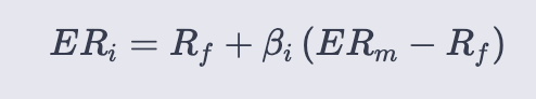
ER = Expected return of the asset

ERm = Expected return of the market portfolio (e.g., S&P 500)

Rf = Risk‑free rate (the notebook uses the 10‑year Treasury yield)

β = Asset beta — the sensitivity of the asset’s excess return to the market’s excess return (estimated here by OLS on excess returns for DPZ daily and XOM monthly)

(ERm − Rf) = Market risk premium

import re
from io import StringIO
from datetime import datetime, timedelta
import requests
import pandas as pd
import numpy as np
import pandas_datareader as pdr
from datetime import datetime
import statsmodels.api as sm
import statsmodels.formula.api as smf

You’re bringing in a set of standard utilities for fetching data, parsing text and dates, manipulating tabular data and arrays, and running statistical models. I’ll walk through what each import gives you and why it’s commonly used, in plain terms.

- re: the regular-expression module. Use it to find or replace patterns in text, validate strings, or split/clean messy textual data.

- StringIO from io: gives you an in-memory text stream that behaves like a file. Handy when you fetch CSV or other text over the network and want to hand it to pandas.read_csv without writing a file to disk.

- datetime and timedelta from datetime: datetime is the object for timestamps (year/month/day/hour/etc.), timedelta represents time differences (add/subtract days, hours, etc.). Together they let you do date arithmetic and format or parse date/time values. (Note: datetime is imported twice in these lines — once together with timedelta, and then again by itself. That second import is redundant but harmless.)

- requests: a simple HTTP client. You use requests.get/post to download a web page or raw CSV text from a URL before turning it into a pandas DataFrame or passing it through StringIO.

- pandas as pd: the core tabular-data library. DataFrames, Series, CSV/Excel/JSON I/O, groupby, merge, resample and lots of convenience for cleaning and transforming data.

- numpy as np: numerical arrays and math functions. Often used alongside pandas for vectorized calculations, array ops, and numerical utilities.

- pandas_datareader as pdr: a convenience layer to fetch financial and economic time series from remote providers (Yahoo, FRED, etc.). It returns pandas objects directly.

- statsmodels.api as sm and statsmodels.formula.api as smf: two entry points into statsmodels. sm is the lower-level API where you typically work with arrays/matrices (and explicitly add an intercept column, etc.). smf provides a formula-style interface (“y ~ x1 + x2”) similar to R, which is compact and convenient for regression specification. Keeping both is common: use smf for quick OLS via formulas, and sm when you need finer control or different model classes.

A couple of small practical notes you’ll feel when running code that uses these imports:

- The aliasing (pd, np, pdr, sm, smf) is just shorthand so the code reads cleanly.

- Importing datetime twice is unnecessary; best practice is to import it once to avoid confusion.

- These import lines don’t themselves produce output — they just make functions and classes available for the rest of your code to call.

# Loading in our data
def get_historical_Data(tickers):
    “”“
    This function returns a pd dataframe with all of the adjusted closing information
    “”“
    data = pd.DataFrame()
    names = list()
    for i in tickers:
        data = pd.concat([data,pdr.get_data_yahoo(symbols=i, start=datetime(2010, 11, 17), end=datetime(2020, 11, 17)).iloc[:,5]], axis = 1)
        names.append(i)
    data.columns = names
    return data

The function builds a table of adjusted closing prices for whatever tickers you hand it, by pulling each ticker’s history from Yahoo and stacking those single-series results side-by-side into one DataFrame.

- Creates an empty DataFrame called data and an empty list names to keep track of the tickers we add.

- Loops over the tickers argument. For each ticker i it calls pdr.get_data_yahoo(…) with fixed start and end dates (datetime(2010,11,17) to datetime(2020,11,17)). From the DataFrame that get_data_yahoo returns it selects .iloc[:,5] — the sixth column — which in the typical Yahoo output is the “Adj Close” series (that is, the adjusted closing price for each date).

- Concatenates that single-column series onto the running data DataFrame along axis=1, so each ticker becomes its own column. The ticker symbol i is appended to names.

- After the loop finishes it sets data.columns = names so the columns are labeled with the ticker symbols you passed in, and returns that DataFrame.

Some practical notes and small caveats to keep in mind:

- The function uses fixed start/end dates; every call will request the same 2010–11–17 to 2020–11–17 window unless you change the code.

- Using .iloc[:,5] assumes the returned Yahoo DataFrame has the adjusted close as its sixth column. That’s usually true, but a more robust approach is to select by column name (“Adj Close”) to avoid index-position fragility.

- Concatenating inside the loop works but is not the fastest pattern for many tickers; an alternative is to collect the series in a list or dict and call pd.concat once at the end.

- pd.concat with axis=1 aligns rows by the date index, so if some tickers have different available dates you’ll get NaNs where a ticker lacks a value for a given date.

In everyday use, calling get_historical_Data([‘DPZ’,’^GSPC’]) (for example) gives you a DataFrame indexed by trading dates with two columns, ‘DPZ’ and ‘^GSPC’, each containing the adjusted close prices for the specified period.

# Reading in our 10 year Treasury Constant Maturity Rate.
# https://fred.stlouisfed.org/series/DGS10
T_rate = pd.read_csv(’DGS10.csv’)

The two lines starting with # are comments telling you what the file contains (the 10‑year Treasury Constant Maturity Rate from FRED) and giving the FRED series URL. The executable line calls pandas.read_csv to open the file ‘DGS10.csv’ and load its contents into a pandas DataFrame assigned to the name T_rate.

read_csv will, by default, treat the first row of the CSV as column names, infer data types for each column, and create a new integer RangeIndex for the rows (so nothing is used as the DataFrame index unless you explicitly ask for it). Because no extra arguments are given, dates in any column will be read as plain strings rather than pandas datetime objects, and missing or unusual values will be handled by pandas’ default NA parsing rules. If the file is not in the current working directory or the path is wrong, Python will raise a FileNotFoundError when this line runs.

After this runs you have the CSV loaded into memory as T_rate and can inspect or manipulate it. Common next checks are:

- T_rate.head() to see the first few rows and confirm column names and sample values

- T_rate.info() to check dtypes and non-null counts

- T_rate.describe() for a quick numeric summary

If you want the date column parsed as datetimes right away, you can add parse_dates=[‘<date-column-name>’] to read_csv, or convert it afterward with pd.to_datetime.

T_rate[’DATE’] = pd.to_datetime(T_rate[’DATE’], format = “%Y-%m-%d”).dt.strftime(’%m-%d-%Y’)

This line takes the DATE column in the T_rate DataFrame, parses those values as datetimes assuming they are written as “YYYY-mm-dd”, then reformats each date into the string form “mm-dd-YYYY” and writes that back into the same column. Concretely, pd.to_datetime(…) turns the column into pandas Timestamp values (datetime64[ns]) using the explicit format argument to interpret the input correctly, and the .dt.strftime(‘%m-%d-%Y’) produces string representations like “01–15–2020” for January 15, 2020.

Broken down:

- pd.to_datetime(T_rate[‘DATE’], format=”%Y-%m-%d”) parses the original strings into datetime objects according to the specified input format.

- .dt.strftime(‘%m-%d-%Y’) converts those datetime objects into strings formatted as month-day-year.

- The assignment at the left replaces the original column with these formatted strings.

A couple of practical notes: because a specific format is supplied, any date string that doesn’t match “%Y-%m-%d” will cause an error (unless you pass errors=’coerce’). After this runs, the DATE column contains formatted strings (object dtype), not pandas datetime objects, so if you later need to do date arithmetic or resampling you would want to keep or recreate a datetime dtype instead.

T_rate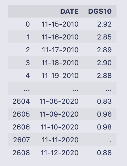

The cell simply evaluated the variable T_rate and printed its contents as a DataFrame. You can read that table as two columns:

- DATE: strings formatted like “mm-dd-YYYY” (examples shown: 11–15–2010, 11–16–2010, …). The DataFrame is using the default integer index (0, 1, 2, …).

- DGS10: values that look like treasury yields (e.g. “2.92”, “2.85”, “2.89”, …). Near the end you can see one entry that is just a dot (“.”) — that’s a non‑numeric placeholder for a missing value.

The printed output shows the first few rows and the last few rows with an ellipsis in between, and the footer reports the full shape: 2609 rows × 2 columns. Because the DGS10 column contains string-formatted numbers and at least one “.”, you won’t be able to do numeric calculations on it until you convert those entries to numeric types and decide how to handle the missing value. Likewise, DATE is currently a string column, so if you need to do date arithmetic or merges by date you’d typically convert it to a datetime type.

count = 0
for i in T_rate[’DGS10’]:
    if i ==’.’:
        T_rate[’DGS10’][count] = T_rate[’DGS10’][count-1]
    count+=1

This loop walks down the DGS10 column one value at a time and replaces any string ‘.’ entries with the previous row’s value — in other words it’s trying to forward-fill missing entries that were encoded as ‘.’.

- count = 0 initializes a simple integer counter that tracks the current row position.

- for i in T_rate[‘DGS10’]: iterates over the values in the Series T_rate[‘DGS10’]. On each pass i is the current cell value (a string or number).

- if i == ‘.’: checks whether the current cell is the placeholder ‘.’.

- T_rate[‘DGS10’][count] = T_rate[‘DGS10’][count-1] copies the previous row’s DGS10 value into the current row when the current value is ‘.’.

- count += 1 increments the counter so the next loop iteration targets the next row.

A few things to be aware of while reading this:

- Because count starts at 0, if the very first element is ‘.’ the code will evaluate T_rate[‘DGS10’][count-1] as T_rate[‘DGS10’][-1]. In Python/pandas that refers to the last element, so the first-row ‘.’ would get replaced by the final row’s value — probably not what you want.

- The expression T_rate[‘DGS10’][count] uses chained indexing (Series selection followed by integer indexing). In pandas this can produce a SettingWithCopyWarning and may sometimes not modify the original DataFrame in-place the way you expect. The code will usually work, but it’s fragile and can lead to subtle bugs or warnings.

After the loop finishes, any ‘.’ entries (except the pathological first-row case) will have been overwritten by the immediately preceding valid value, so the column ends up with those placeholders replaced by the prior observed value.

#    The ticker names of the companies that we will be looking at. (And the S&P500)
ticks = [”DPZ”, ‘^GSPC’]
d = get_historical_Data(ticks)

The first line creates a small list called ticks that holds the symbols we want to pull: “DPZ” (Domino’s Pizza) and “^GSPC” (the Yahoo Finance symbol for the S&P 500 index). That list is just a simple Python list of strings — it’s telling the data-fetching function which series to grab.

- columns named “DPZ” and “^GSPC” containing the adjusted close price values,

- the index made up of the datetime values for each observation,

- numeric price values (with possible NaNs if data is missing for some dates).

A quick way to check what you got is to look at d.head(), d.tail(), or d.info() — that will show the date range, any missing values, and the column names so you know the next steps (computing returns, merging with other tables, plotting, etc.). Also be aware that fetching data requires internet access and can fail or return NaNs if the service is unavailable or if ticker symbols are invalid.

print(d.shape)
#

print(d.shape) asks Python to report the dimensions of the object d. For a pandas DataFrame, the .shape attribute is a two-element tuple: (number_of_rows, number_of_columns), and print(…) writes that tuple to the notebook output.

- 2,518 is the number of observations (one per row).

- 2 is the number of variables/series stored as columns.

Seeing this number is a quick sanity check: you can tell at a glance how many data points you have and that you actually have two series available. Typical next checks after this would be to look at d.columns to see the column names and d.head() / d.tail() to inspect the first and last rows, or to look for missing values, but the printed shape itself just confirms the size of the DataFrame.

d = d.reset_index()
for i in range(d.shape[0]):
    mo = ‘’
    da = ‘’
    if d[’index’][i].month < 10:
        mo = ‘0’ + str(d[’index’][i].month)
    else:
        mo = str(d[’index’][i].month)
    if d[’index’][i].day < 10:
        da = ‘0’ + str(d[’index’][i].day)
    else:
        da = str(d[’index’][i].day)
    d[’index’][i] = mo + ‘-’ + da + ‘-’ + str(d[’index’][i].year) 
# Changing the index name to date
d = d.rename(columns = {”index”: “DATE”})

The code is taking whatever was the DataFrame index (a DatetimeIndex) and turning those timestamps into strings in the format “mm-dd-YYYY”, then renaming that column to “DATE”. Concretely:

- d = d.reset_index() moves the existing index into a regular column named “index” and gives the DataFrame a new integer index. The values in d[‘index’] are Timestamp objects (datetime-like).

- The for loop walks every row index i and builds two strings mo and da for month and day. If month or day is less than 10 it prepends a “0” so you get two-digit months/days (e.g. 03, 09). It then constructs mo + ‘-’ + da + ‘-’ + year and assigns that string back into d[‘index’][i]. In other words, each Timestamp is converted to a string like “03–09–2021”.

- After the loop finishes, d = d.rename(columns = {“index”: “DATE”}) simply renames the column to DATE.

So the intent and end result: the original datetime index values become a column of zero-padded mm-dd-YYYY strings saved as DATE.

The warning you see is pandas’ SettingWithCopyWarning, produced at the line that writes d[‘index’][i] = …. That warning means pandas is unsure whether your assignment is modifying the original DataFrame or just a temporary view/copy — chained/index-based assignment like d[‘index’][i] can be ambiguous and is discouraged. The practical risks are: your assignment might not persist in all situations, and the code is inefficient.

Two practical improvements:

- Use vectorized datetime formatting (fast and robust), for example:

- d[‘DATE’] = d[‘index’].dt.strftime(‘%m-%d-%Y’)

- then drop or rename the original index column if you want.

This avoids explicit Python loops and the SettingWithCopyWarning.

- If you prefer to keep the loop approach, assign with .loc to avoid the warning:

- d.loc[i, ‘index’] = formatted_string

but vectorized dt.strftime is still the preferred method for performance and clarity.

So functionally the code works to produce mm-dd-YYYY strings, but the warning points out a safer and faster way to do it.

d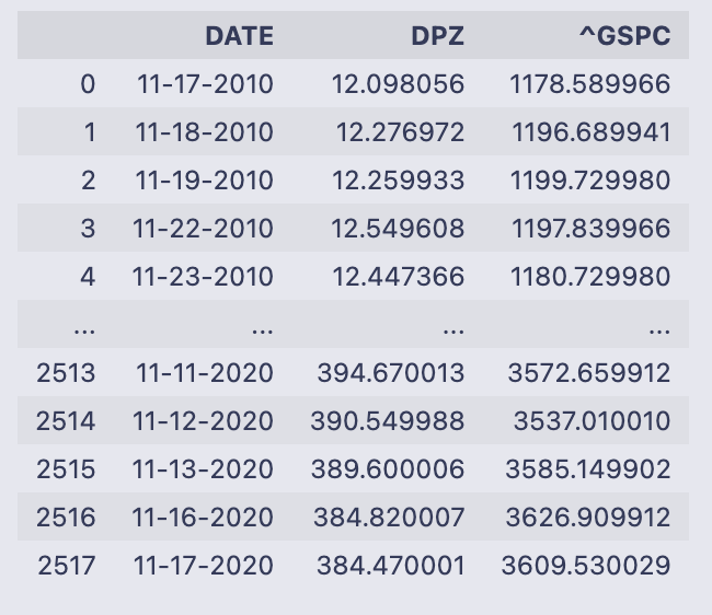

When you evaluate the name d in a notebook cell, Jupyter displays the contents of that pandas DataFrame. What you see here is a three-column table with 2,518 rows. The leftmost column shown in the display (0, 1, 2, …) is the DataFrame’s integer row index; the table itself has these columns:

- DATE — strings formatted like “11–17–2010”, “11–18–2010”, etc., so each row represents a trading date.

- DPZ — numeric values (floats) for the first series; those look like per-share prices or levels (e.g., 12.098056 on 11–17–2010).

- ^GSPC — numeric values (floats) for the second series; these are index-level numbers (e.g., 1178.589966 on 11–17–2010).

The printout shows the first five rows and the last five rows of the frame (a typical truncated display for a large DataFrame). The earliest date visible is 11–17–2010 and the latest shown is 11–17–2020, so this is a roughly ten-year daily time series. The small text summary at the bottom confirms the shape: [2518 rows x 3 columns].

So at a glance, d holds two time-aligned numeric series indexed by date strings, ready for further operations such as computing percent changes, merging with other tables, or feeding into a regression.

# Merge dataframes
data = pd.merge(left = T_rate, right = d, left_on = ‘DATE’, right_on = ‘DATE’)
data = data.rename(columns = {”DGS10”: “10_Year_Rate”})

The first line performs a table join: pd.merge takes the two DataFrame objects T_rate (the left table) and d (the right table) and matches rows where the values in their DATE columns are equal. Because you passed left_on=’DATE’ and right_on=’DATE’, those columns are used as the key for the join. By default pd.merge does an inner join, so the resulting DataFrame (assigned to data) will contain only rows where the DATE value existed in both T_rate and d. The merged result contains all columns from both inputs (the DATE key plus the other columns from each frame).

The second line just renames one column in that merged DataFrame: rename({“DGS10”: “10_Year_Rate”}) replaces the column name “DGS10” with the more descriptive “10_Year_Rate”. rename returns a new DataFrame, so assigning it back to data updates the variable with that column-name change. T_rate and d themselves are not modified by these operations; data is a new DataFrame that combines their columns and uses the renamed treasury-rate column.

data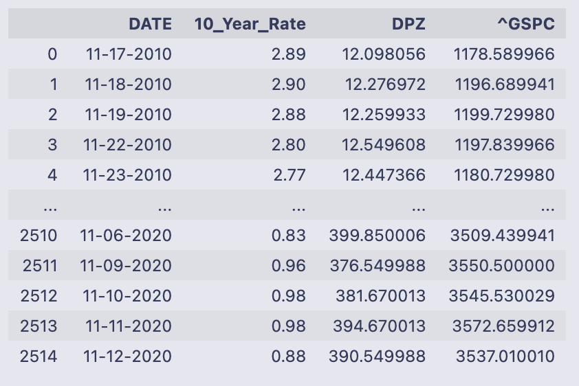

The output is the printed contents of the DataFrame named data — pandas shows the first few rows and the last few rows with an ellipsis in the middle because the table is large. You can read down the columns to see what each row contains for a single date.

- DATE: a string-formatted date (looks like mm-dd-YYYY). The first rows shown are mid-November 2010 and the last rows shown are November 2020, so the table spans about ten years. The DataFrame index on the left is the default integer RangeIndex (0 up to 2514).

- 10_Year_Rate: numeric values like 2.89, 2.90, down to values below 1.0 near the end of the sample — this is the 10-year Treasury yield expressed in percentage points (e.g., 2.89 means 2.89%).

- DPZ and ^GSPC: floating-point numbers with many decimals. Those are price series (DPZ is the company price column, ^GSPC is the market/index price column). Over the displayed period DPZ moves from around 12 to around 390, and ^GSPC moves from about 1,178 to about 3,537, showing substantial price appreciation across the sample.

At the bottom of the text output you see the DataFrame shape: [2515 rows x 4 columns], confirming there are 2,515 date-observations and the four fields listed above. The printed preview is just a snapshot — if you want to inspect particular rows, columns, or dtypes you can call data.head(), data.tail(), data.shape, or data.dtypes to get exact types and a focused view.

# Because of the CAPM formula, we need to calculate the Percent changes of our given assets.
data[’DPZ_Daily_Returns’] = data[’DPZ’].pct_change()
data[’SP500_Daily_Returns’] = data[’^GSPC’].pct_change()

These two lines add daily return columns to the data DataFrame by computing the percent change in the adjusted prices for each asset. The pct_change() method on a pandas Series calculates (current_value — previous_value) / previous_value for each row, so you get the fractional change from one observation to the next.

Concretely:

- data[‘DPZ_Daily_Returns’] is the sequence of day-to-day returns for the DPZ price series stored in data[‘DPZ’].

- data[‘SP500_Daily_Returns’] is the same idea for the S&P 500 series stored in data[‘^GSPC’].

A few practical notes you’ll see when you inspect these columns:

- The first entry will be NaN because there is no prior price to compute the change against.

- The numbers are in decimal form (e.g., 0.02 means a 2% increase). If you need percentage points, multiply by 100.

- pct_change() uses the DataFrame’s index to line up consecutive rows, so the return at row i compares the value at i with the value at i-1.

- If a previous value is zero or non-numeric, pct_change can produce infinities or NaNs, so make sure the price columns are clean numeric series before calling it.

Because the comment mentions CAPM, these return series are what you’d feed into any excess-return or regression steps that follow: they represent the realized daily returns that CAPM-style calculations typically use.

data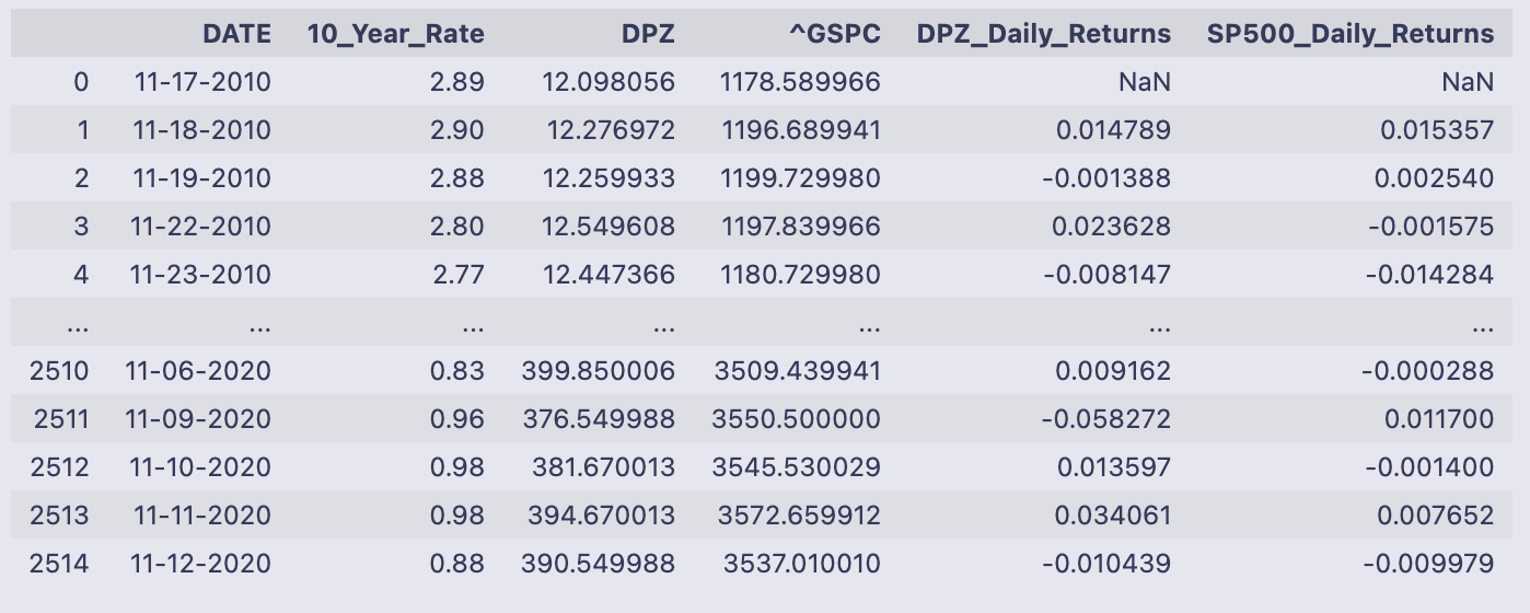

The variable data printed here is a pandas DataFrame snapshot. It has six columns and 2,515 rows (index running 0 to 2514), and the output shows the first few rows and the last few rows so you can see how the values evolve over time.

The columns are:

- DATE: a date string for each row (formatted like “11–17–2010”); note the DataFrame keeps the date values in a column rather than as the index.

- 10_Year_Rate: a number that looks like a percentage rate (e.g., 2.89, 2.90, 0.83).

- DPZ: a price series for the DPZ instrument (starts around 12.10 in the first row and rises to ~390 by the last rows shown).

- ^GSPC: the S&P 500 index level (starts ~1,178 and is ~3,537 near the end).

- DPZ_Daily_Returns: the day-over-day percent change of the DPZ price; the first row is NaN because there is no prior day to compute a change.

- SP500_Daily_Returns: the day-over-day percent change of the S&P 500 column; likewise the first row is NaN.

Looking at the numeric samples, you can see how the rate and prices evolve across the ten-year-ish span shown: DPZ grows from low double-digits to the high hundreds, the S&P500 grows from ~1,100 to ~3,500, and the 10_Year_Rate declines from roughly 2.9% to under 1% in the final rows shown. The returns columns are small decimals (e.g., 0.0148 ≈ 1.48% for DPZ on 11–18–2010), which is exactly what you would expect from percent-change calculations. The plain-text and HTML representations in the output are just pandas’ default ways of showing the DataFrame.

# Taking out the first row as it is NaN
data = data[1:]

# Calculate the excess return

data[’Excess_Return_DPZ’] = data[’DPZ_Daily_Returns’] - data[’10_Year_Rate’].astype(’float’) / 100
data[’Excess_Return_SP500’] = data[’SP500_Daily_Returns’] - data[’10_Year_Rate’].astype(’float’) / 100

The first line removes the very first row from data (data = data[1:]) because that row contains NaN values from the prior percent-change calculation — the comment explains that. After that you compute two new columns, Excess_Return_DPZ and Excess_Return_SP500, by subtracting the risk-free rate (the 10_Year_Rate column) from each asset’s returns. The code converts 10_Year_Rate to float and divides by 100, so you’re turning a percentage like “1.50” into a decimal 0.015 before subtracting it from the return series.

Both subtraction lines are vectorized operations: pandas aligns the series by index and does the arithmetic element-wise, producing two new Series that get stored as columns in data.

The output shows a pandas SettingWithCopyWarning for both assignments. That warning means pandas thinks data might be a view of another DataFrame (because data = data[1:] produces a slice) and not a fully independent copy, so assigning new columns could have unintended behavior or might not modify the original object you expect. It’s a caution, not an exception, but you should resolve it to avoid subtle bugs.

A few practical ways to fix this:

- Make an explicit copy of the sliced frame before assigning new columns (recommended).

- Use .loc to do the assignment explicitly (can also help).

- Ensure the risk-free-rate column is numeric before arithmetic (astype(‘float’) usually works; pd.to_numeric(…, errors=’coerce’) is safer if there may be non-numeric strings).

Example fixes you can drop in place of the original lines:

- Create a copy first:

data = data[1:].copy()

data[‘Excess_Return_DPZ’] = data[‘DPZ_Daily_Returns’] — data[‘10_Year_Rate’].astype(float) / 100

data[‘Excess_Return_SP500’] = data[‘SP500_Daily_Returns’] — data[‘10_Year_Rate’].astype(float) / 100

- Or use .loc and ensure numeric conversion:

data = data.iloc[1:] # keep the slice

data.loc[:, ‘Excess_Return_DPZ’] = data[‘DPZ_Daily_Returns’] — pd.to_numeric(data[‘10_Year_Rate’], errors=’coerce’) / 100

data.loc[:, ‘Excess_Return_SP500’] = data[‘SP500_Daily_Returns’] — pd.to_numeric(data[‘10_Year_Rate’], errors=’coerce’) / 100

Either approach removes the warning and makes it explicit that you’re modifying a concrete DataFrame. The numeric conversion step makes sure the subtraction uses decimal risk-free rates (e.g., 0.015) rather than leftover strings.

data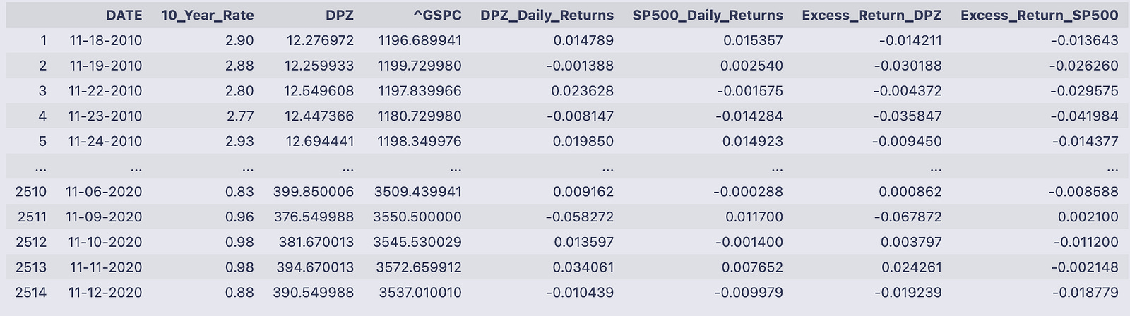

You’re looking at the pandas DataFrame named data printed to the notebook output. It has 2,514 rows and eight columns; each row is a dated observation (the DATE column holds strings like 11–18–2010) and the integer index down the left runs from 1 to 2514 in the printed view.

The eight columns are:

- DATE: the observation date as a string in mm-dd-YYYY format.

- 10_Year_Rate: a numeric-looking value (e.g., 2.90, 0.83) that represents the 10-year Treasury rate on that date.

- DPZ and ^GSPC: the adjusted close prices for two assets (DPZ and the S&P 500 index) shown as floating point numbers.

- DPZ_Daily_Returns and SP500_Daily_Returns: the day-to-day returns for those price series, shown as decimal fractions (for example 0.014789 ≈ 1.4789%).

- Excess_Return_DPZ and Excess_Return_SP500: the returns that remain after adjusting for the 10_Year_Rate (so they’re smaller decimal numbers, positive or negative depending on whether the asset outperformed that rate that day).

Read a single-row example to see how the pieces fit together. On 11–18–2010 the DPZ price was 12.276972 and the S&P index was 1196.689941; the DPZ daily return is 0.014789 (≈1.48%) and the S&P return is 0.015357 (≈1.54%). The Excess_Return_DPZ shown that day is -0.014211, meaning DPZ’s return minus the benchmark risk-free rate produced a negative excess on that date.

The output is truncated in the middle with “…” (standard pandas display), showing the first few and last few rows so you can check structure and sample values without printing all 2,500+ rows. The final printed line confirms the shape: 2514 rows × 8 columns. Overall, the table gives you the raw prices, computed daily returns, the prevailing 10-year rate at each date, and the asset returns expressed net of that rate.

# Running a regression to calculate Beta
results = smf.ols(’Excess_Return_DPZ ~ Excess_Return_SP500’, data = data).fit()

We’re asking statsmodels’ formula interface to run a simple ordinary least squares regression and store the fitted model in the variable results.

Breaking the line down:

- smf.ols(…) is the OLS (ordinary least squares) constructor from statsmodels.formula.api. It takes a formula string and a DataFrame. The formula ‘Excess_Return_DPZ ~ Excess_Return_SP500’ tells patsy/statsmodels that Excess_Return_DPZ is the dependent variable and Excess_Return_SP500 is the single predictor. By default an intercept term is included.

- data = data tells the function where to find the named columns — the DataFrame must contain columns named exactly ‘Excess_Return_DPZ’ and ‘Excess_Return_SP500’. Any rows with missing values in those columns will be excluded from the fit.

- .fit() actually performs the regression: it builds the design matrix, computes coefficient estimates that minimize the sum of squared residuals, and computes associated statistics (standard errors, t-stats, etc.). The result of .fit() is a fitted model object (a RegressionResultsWrapper) and that’s what gets assigned to results.

- results.params gives the estimated coefficients (intercept and slope).

- results.fittedvalues are the model predictions; results.resid are residuals (observed minus fitted).

- results.rsquared and results.rsquared_adj are measures of fit; results.pvalues and results.bse give p-values and standard errors.

- results.summary() prints a full regression table with coefficients, t-stats, p-values, R-squared, and diagnostic info.

So after this line runs you have a fitted linear model object in results that you can inspect, summarize, or use to predict, plot residuals, etc.

print(results.summary())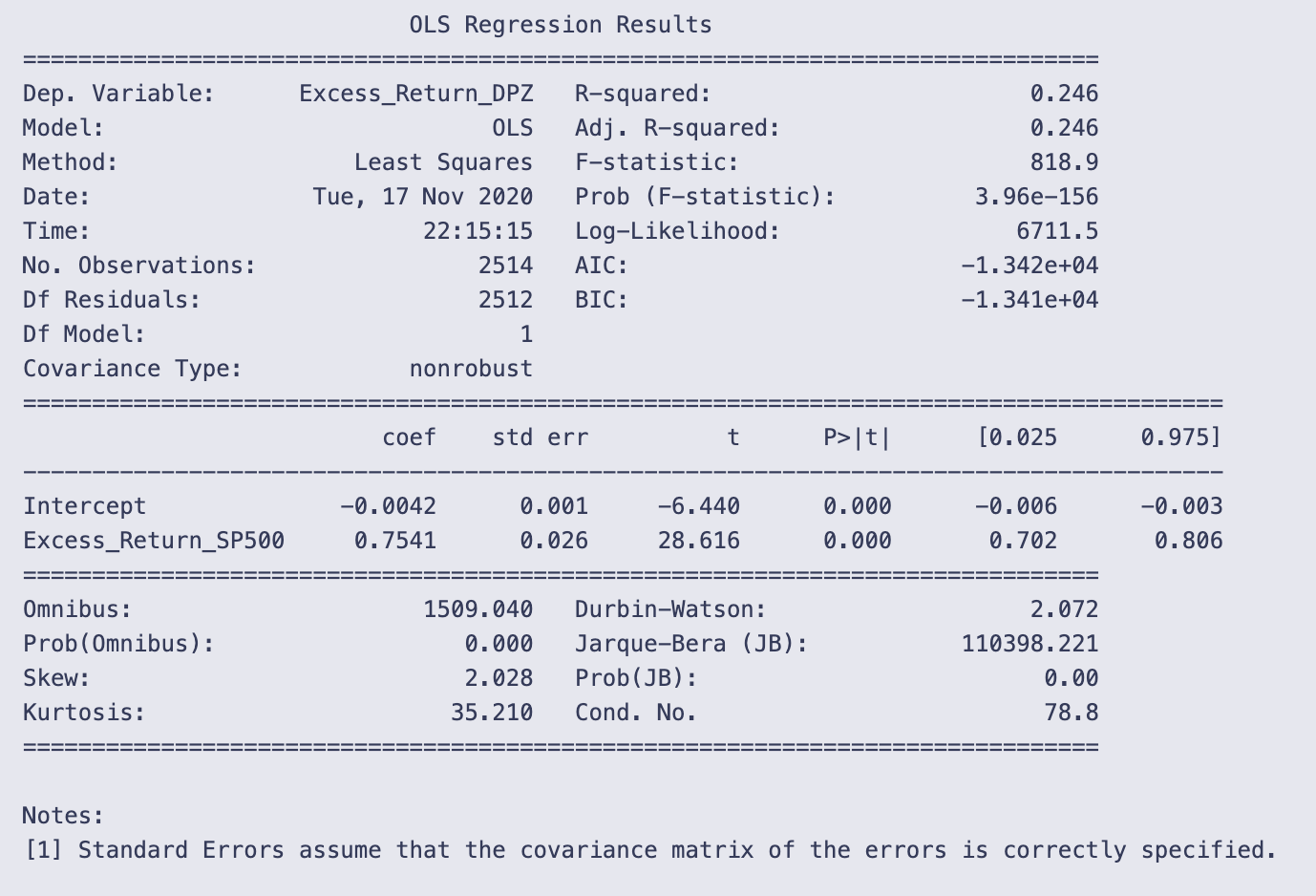

You’re calling statsmodels’ summary printer on a fitted OLS result object and getting the human-readable regression report printed to the notebook. That single line, print(results.summary()), asks the results object to format a full set of model statistics and then sends that formatted text to standard output. The output you see is that formatted report.

A quick walk through what the report is telling you and how to read it:

- Top block (model and fit statistics): it names the dependent variable (Excess_Return_DPZ), the model (OLS), the number of observations (2514), and goodness-of-fit measures. R-squared = 0.246 means the model explains about 24.6% of the variation in the dependent variable. The F-statistic (818.9) and its tiny p-value (3.96e-156) indicate the model as a whole is statistically significant (i.e., the predictor improves fit relative to a model with only a constant).

- Coefficient table (the core of the regression): there are two rows, Intercept and Excess_Return_SP500, and several columns:

- coef: Intercept = -0.0042 and the slope on Excess_Return_SP500 = 0.7541. In plain terms, the slope says that for a one-unit increase in Excess_Return_SP500, the dependent variable Excess_Return_DPZ is estimated to increase by about 0.7541 units (in whatever units the returns are measured).

- std err, t, and P>|t|: both coefficients are highly statistically significant (large t-statistics, p-values reported as 0.000), so the slope is very unlikely to be zero given the data.

- [0.025 0.975]: the 95% confidence interval for the slope is approximately [0.702, 0.806], so the estimate is fairly precisely centered around 0.75.

- Diagnostic numbers at the bottom: these help check assumptions.

- Durbin-Watson ≈ 2.072 is close to 2, which suggests little evidence of first-order autocorrelation in the residuals.

- Omnibus and Jarque-Bera tests have huge statistics and p-values ~0.000, and kurtosis = 35.21 with positive skew. That combination indicates the residuals are far from normally distributed (heavy tails and skew). Non-normal residuals don’t bias coefficient estimates but do affect inference (standard errors, p-values) if not accounted for.

- Cond. No. = 78.8 is modest; with only one predictor this doesn’t suggest multicollinearity is a concern.

A couple of practical takeaways: the predictor (Excess_Return_SP500) is strongly associated with the response and explains a meaningful fraction of its variance, but the residuals show strong non-normality (very heavy tails). Also note the small-print reminder at the bottom that standard errors assume the covariance matrix is correctly specified; if residuals violate assumptions (heteroskedasticity, heavy tails), you might want robust standard errors or other diagnostics before relying blindly on p-values.

# Beta from the OLS above
Beta = 1.1367
# Once we have Beta, we can calculate the expected return of the company BASED on the market.
average_risk_free_rate = data[’10_Year_Rate’].astype(’float’).mean() /100
# Using the Historical Rate of return for the S&P500 market...
# Including dividends but not accounting for inflation
average_return_SP500 = (1.311 * (1-.0441) * (1.2194) * (1.1193) * (1.0131) * (1.1381))**(1/5) - 1

print(’Average Risk Free Rate’,average_risk_free_rate)
print(’Average Return S&P500’,average_return_SP500)
print(’Expected Return of DPZ’,average_risk_free_rate + Beta * (average_return_SP500 - average_risk_free_rate))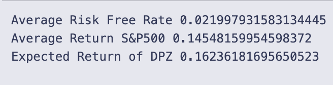

Beta is set to 1.1367 — that scalar is the sensitivity of the stock to the market used in the CAPM formula.

average_risk_free_rate = data[‘10_Year_Rate’].astype(‘float’).mean() / 100 takes the 10-year rate values stored in data, forces them to floats, computes their mean, and divides by 100 so the rate becomes a decimal (for example 0.02 for 2%). This is the risk-free rate used in the CAPM calculation.

average_return_SP500 is computed as a geometric average of five yearly gross return factors:

(1.311 * (1 — .0441) * 1.2194 * 1.1193 * 1.0131 * 1.1381) ** (1/5) — 1.

Each factor like 1.311 or (1 — .0441) is a gross return for one year (1 + yearly return, with a negative year shown as 1–0.0441). Multiplying them gives total growth across the period, raising to the 1/5 power gives the average annual gross growth, and subtracting 1 converts that back to an average annual return. The inline comment notes these numbers include dividends but are not adjusted for inflation.

- Average Risk Free Rate 0.021997931583134445 → about 2.20%

- Average Return S&P500 0.14548159954598372 → about 14.55%

- Expected Return of DPZ 0.16236181695650523 → about 16.24%

The expected return is computed with the CAPM formula:

Expected = Rf + Beta * (Rm — Rf).

Plugging the printed numbers in: Rf ≈ 0.021998, Rm ≈ 0.145482, Beta = 1.1367. The market risk premium (Rm — Rf) ≈ 0.123484; multiplying by Beta gives the stock’s compensated premium, and adding Rf yields the final expected return ≈ 0.16236 (16.24%). Because Beta > 1, this stock’s expected excess return is amplified relative to the market’s excess return.

Apply the same CAPM workflow to the monthly series — XOM versus the S&P 500 (uses Monthly_DGS10.csv)

# Using Monthly data for T Rates
mT_rate = pd.read_csv(’Monthly_DGS10.csv’)
#https://fred.stlouisfed.org/series/DGS10
count = 0
for i in mT_rate[’DGS10’]:
    if i ==’.’:
        mT_rate[’DGS10’][count] = mT_rate[’DGS10’][count-1]
    count+=1
mT_rate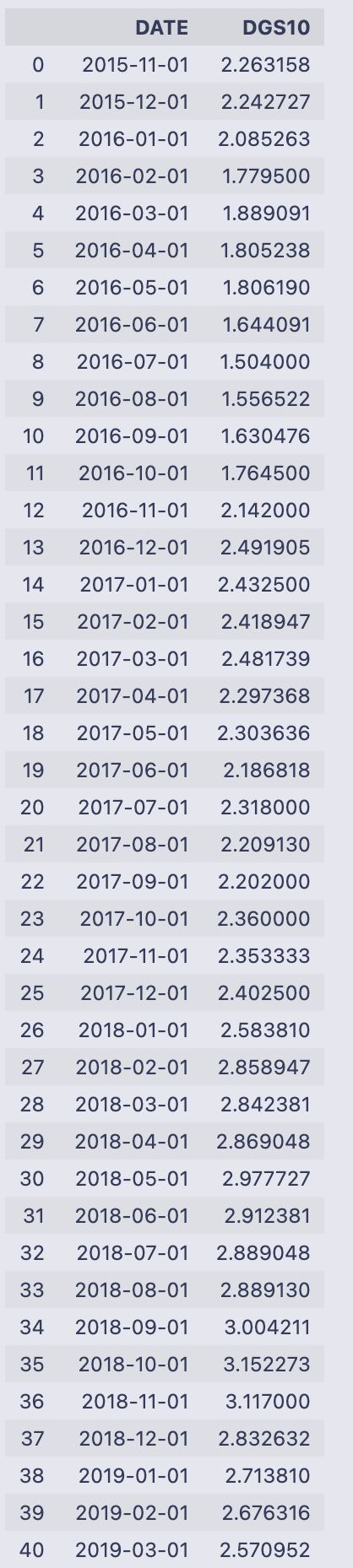

It reads the file Monthly_DGS10.csv into a pandas DataFrame called mT_rate so the variable holds the table of dates and the 10‑year rate column labeled “DGS10”. Then the code walks through the DGS10 column value by value using a manual counter (count starts at 0 and increments each loop). For every entry i it checks if i is the string ‘.’ and, if so, assigns the previous row’s DGS10 value into the current row via mT_rate[‘DGS10’][count] = mT_rate[‘DGS10’][count-1]. That is a simple forward-fill-by-one approach: any placeholder ‘.’ is replaced in place with whatever value appeared immediately above it. Finally the DataFrame is returned/printed, so you see the DATE and DGS10 columns.

The printed output shows DATEs from 2015–11–01 through 2020–10–01 and numeric-looking DGS10 values (e.g. 2.263158, 2.242727, …, 0.787143). Because no ‘.’ placeholders appear in the displayed DGS10 column, nothing visibly changed in this run — the loop simply inspected each element and didn’t perform any replacements.

A couple of practical notes to keep in mind when you read this pattern: iterating a pandas Series with a separate counter and assigning with mT_rate[‘DGS10’][count] works but is not the most idiomatic or efficient pandas approach. Also, if the very first entry were ‘.’ the code would try to use count-1 (which is -1) and would end up referencing the last row — an unintended behavior. A more robust method would use pandas methods such as replace + fillna or forward-fill (ffill) or indexing with .loc/.iloc to avoid those pitfalls.

import pandas_datareader.data as web
# Monthly Company data
tick = ‘XOM’
Mdata = web.get_data_yahoo(tick,’11/24/2015’,interval=’m’)
#Monthly Market data
MMdata = web.get_data_yahoo(’^GSPC’,’11/24/2015’,interval=’m’)

You import the Yahoo-finance data reader and give it the short name web so you can call its download function more concisely. Then you set a ticker string for Exxon Mobil (XOM) and ask the reader to fetch monthly price series for that ticker starting on 2015–11–24. A second call asks for the same monthly series for the S&P 500 index (the Yahoo symbol ‘^GSPC’) from the same start date.

Each get_data_yahoo call returns a pandas DataFrame indexed by timestamps (one row per monthly observation because you requested interval=’m’). The usual columns are Open, High, Low, Close, Adj Close and Volume — Adj Close is the inflation/dividend-adjusted closing price most people use for return calculations. The range of rows will run from the given start date up to the most recent data Yahoo provides.

So after these lines you have two DataFrames:

- Mdata: monthly OHLCV + Adj Close for XOM, indexed by date.

- MMdata: monthly OHLCV + Adj Close for the S&P 500, indexed by date.

A couple of practical notes to keep in mind: the date strings you passed determine the starting point (inclusive), and monthly frequency typically gives one observation per month (commonly month-end). Also, these network calls can fail if there’s no internet or if the Yahoo endpoint is temporarily unavailable, in which case you’ll get an exception instead of a DataFrame. To see what you downloaded, call methods like .head(), .columns, or .index on Mdata/MMdata and use the ‘Adj Close’ column if you plan to compute returns.

Mdata = Mdata.rename(columns = {”Adj Close”: tick})
MMdata = MMdata.rename(columns = {”Adj Close”: “SP500”})

You’re relabeling the “Adj Close” column in two DataFrame objects so the column names are more meaningful and easier to work with later.

The first line uses Mdata.rename(columns={“Adj Close”: tick}) to change the column header “Adj Close” to whatever string is stored in the variable tick. Because the result of rename is assigned back to Mdata, the DataFrame Mdata now has that new column name instead of “Adj Close”. A concrete example: if tick holds “XOM”, the column formerly called “Adj Close” becomes “XOM”, and you can refer to it as Mdata[“XOM”] from that point on.

The second line does the same for MMdata, renaming “Adj Close” to “SP500”. After this assignment, MMdata will have a column named “SP500” containing the adjusted close prices.

A few practical notes:

- rename returns a new DataFrame (it does not modify the original in place unless you pass inplace=True), so assigning the result back (Mdata = …) is what actually updates the variable.

- Only the column label is changed; the data in the column and any other columns remain untouched.

- If “Adj Close” isn’t present, rename just leaves the DataFrame unchanged.

- Using clear, ticker-based names avoids ambiguous or duplicate column labels when you later merge or concatenate multiple price DataFrames.

Mdata = pd.concat([Mdata[tick], MMdata[’SP500’] ], axis = 1)

You’re taking two columns (or series) and putting them side-by-side into a new DataFrame, then storing that back into the name Mdata.

- Mdata[tick] looks up the column in Mdata whose name is held by the variable tick and returns a pandas Series. MMdata[‘SP500’] looks up the ‘SP500’ column in MMdata and returns another Series.

- pd.concat([…], axis=1) takes those two Series and concatenates them horizontally (axis=1), aligning rows by their index. That produces a DataFrame with two columns: one named by the value of tick and the other named ‘SP500’.

- The assignment Mdata = … overwrites the previous Mdata object with this new two-column DataFrame.

A couple of practical consequences to keep in mind: the rows are matched by index values (so if the two series have different date indexes you’ll get NaNs where they don’t align), the column order in the result follows the list order you passed to concat, and if the original Mdata had other columns they are discarded because you replace Mdata with only these two columns.

Mdata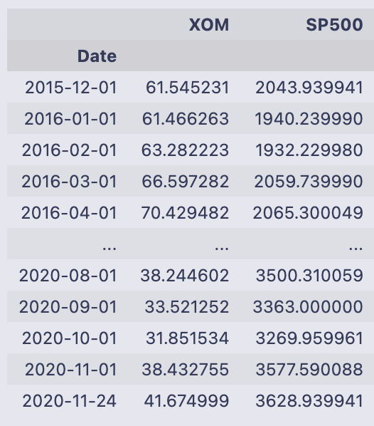

You’re seeing the printed contents of the DataFrame Mdata. The leftmost label (Date) is the index and lists monthly date points from 2015–12–01 through 2020–11–24; pandas shows the first several rows, then “…” for the middle, then the last several rows. The footer “61 rows x 2 columns” tells you the DataFrame has 61 observations and two columns.

The two columns are named XOM and SP500 and contain floating-point numbers — these are the price values for Exxon Mobil (XOM) and the S&P 500 at each date. For example, on 2015–12–01 XOM is about 61.55 and SP500 about 2043.94; by 2020–11–24 XOM is about 41.67 and SP500 about 3628.94. The column names and numeric ranges make it clear these are time-aligned price series sampled monthly.

Printing a variable by itself in a notebook like this calls pandas’ formatted representation, which shows a compact table (head and tail) rather than every row when the table is long. If you want to operate on these values next, typical next steps would be to compute percent changes (returns), reset the index to make the dates a column, or merge these prices with other data indexed by the same dates.

Mdata = Mdata.reset_index()
for i in range(Mdata.shape[0]):
    mo = ‘’
    da = ‘’
    if Mdata[’Date’][i].month < 10:
        mo = ‘0’ + str(Mdata[’Date’][i].month)
    else:
        mo = str(Mdata[’Date’][i].month)
        
    if Mdata[’Date’][i].day < 10:
        da = ‘0’ + str(Mdata[’Date’][i].day)
    else:
        da = str(Mdata[’Date’][i].day)
    Mdata[’Date’][i] = str(Mdata[’Date’][i].year) + ‘-’ + mo  + ‘-’ +  da
# Changing the index name to date
Mdata = Mdata.rename(columns = {”Date”: “DATE”})
Mdata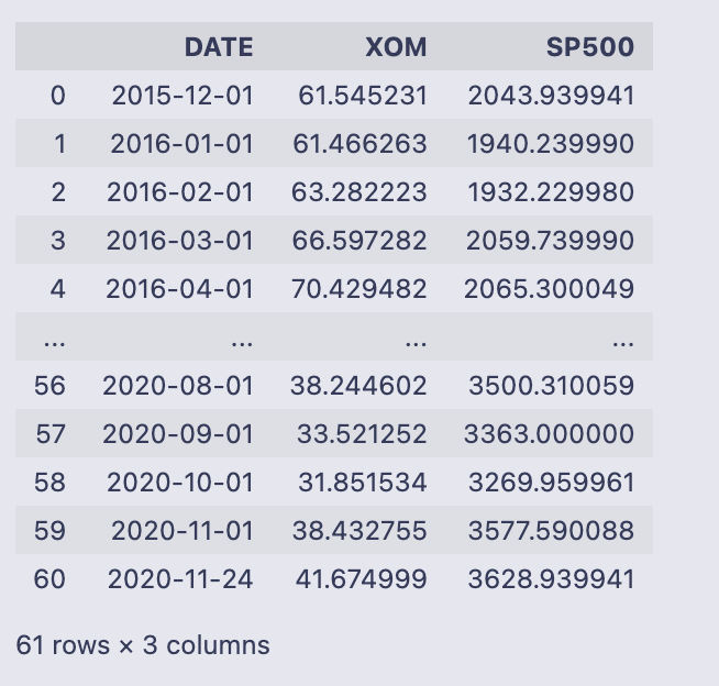

Mdata.reset_index() turns the DataFrame’s index (which was a DatetimeIndex) into a regular column called ‘Date’ so you can format it like any other column. After that the code walks every row with a for loop and builds a YYYY-mm-dd string manually: it checks the month and day, prefixes a ‘0’ when they are single-digit, and then overwrites the value in Mdata[‘Date’][i] with the constructed string. Finally it renames the ‘Date’ column to ‘DATE’ and prints the DataFrame.

- The loop uses range(Mdata.shape[0]) and accesses each cell with Mdata[‘Date’][i]. For each row it constructs mo and da strings (month and day) with leading zeros when needed, then combines them with the year into the format “YYYY-mm-dd”.

- Because the code assigns to Mdata[‘Date’][i] inside the loop, pandas raises a SettingWithCopyWarning. That happens when you may be setting a value on a view rather than the original DataFrame; the result can be unpredictable. The warning is telling you that the assignment might not affect the original DataFrame in the way you expect.

- The final printed DataFrame has three columns: DATE (the formatted strings), XOM, and SP500. There are 61 rows. Most DATE values look like first-of-month strings such as “2016–01–01”, and you can also spot that the last row is “2020–11–24” (not the first of the month) which reflects whatever timestamp was present in the original index for that row.

Two practical improvements to avoid the warning and make the code faster and clearer:

- Use pandas’ datetime formatting methods instead of looping. For example, if ‘Date’ is a datetime dtype, you can do:

Mdata[‘DATE’] = Mdata[‘Date’].dt.strftime(‘%Y-%m-%d’)

then drop the old ‘Date’ column or rename as needed. This is vectorized and much faster.

- If you must set values row-by-row, use .loc or .at to avoid chained indexing:

Mdata.loc[i, ‘Date’] = …

or

Mdata.at[i, ‘Date’] = …

but the vectorized dt.strftime approach is preferred.

So functionally the code converts the index into a column, reformats dates to “YYYY-mm-dd” strings with manual zero-padding, renames that column to ‘DATE’, and prints the resulting DataFrame — but it’s doing that in an inefficient and warning-producing way that is easily replaced with a single vectorized pd.to_datetime/.dt.strftime call.

Mdata[’SP500_Daily_Returns’] = Mdata[’SP500’].pct_change()
Mdata[’{}_Daily_Returns’.format(tick)] = Mdata[tick].pct_change()
Mdata = Mdata[1:]

The first two lines add two new columns to the Mdata DataFrame that contain percent-change returns, and the third line drops the very first row which will be NaN after that calculation.

Mdata[‘SP500_Daily_Returns’] = Mdata[‘SP500’].pct_change()

- This computes the percent change for the values in the ‘SP500’ column from one row to the next. pct_change() calculates (current — previous) / previous for each row and returns a floating-point series (e.g., 0.02 means a 2% change). Because there is no previous row for the very first entry, that first result is NaN, and the new column is added to Mdata.

Mdata[‘{}_Daily_Returns’.format(tick)] = Mdata[tick].pct_change()

- This does exactly the same thing but for whichever column name is contained in the variable tick. The expression ‘{}_Daily_Returns’.format(tick) builds a column name by inserting tick into the string (for example, if tick is ‘XOM’ the new column will be named ‘XOM_Daily_Returns’). That new column holds the percent-change series for Mdata[tick].

Mdata = Mdata[1:]

- After computing percent changes, this slices the DataFrame to drop the first row (index 0). That removes the NaN entries that resulted from pct_change() for both new columns, leaving only rows where the percent change is defined.

A few practical notes to keep in mind: pct_change uses the DataFrame’s row order, so the dates/index must be in chronological order for correct returns; pct_change can produce inf or NaN if the previous value is zero; and the column names include “Daily” purely from the string here, regardless of the actual time frequency of the rows.

# Merging Data Frames
Mdata = pd.merge(left = mT_rate, right = Mdata, left_on = ‘DATE’, right_on = ‘DATE’)
Mdata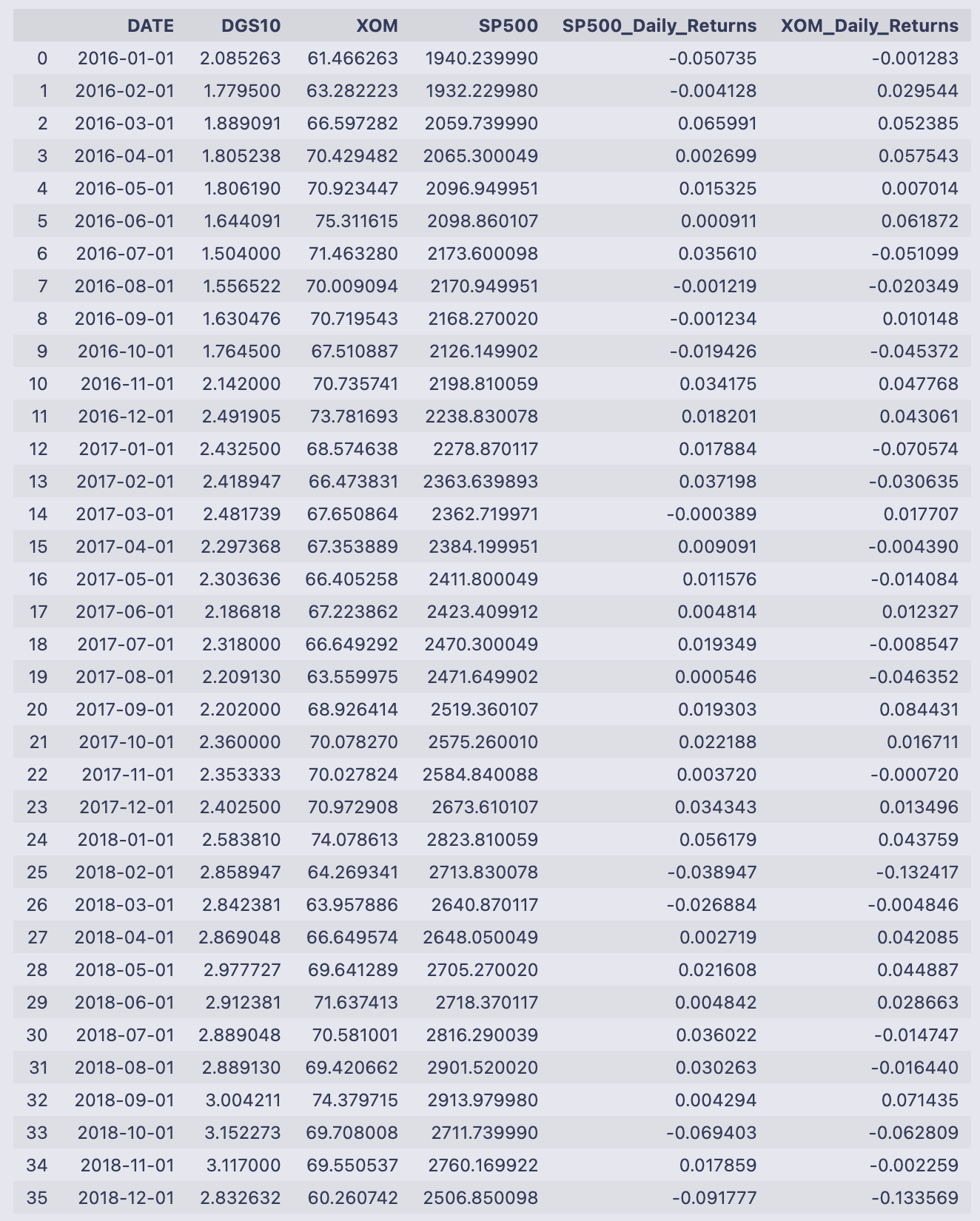

You’re taking two tables that both have a DATE column and gluing them together so each row contains the treasury rate and the monthly price/return info for the same date. The pd.merge call explicitly sets the left table to mT_rate and the right table to Mdata and matches rows where left.DATE == right.DATE. Because no join type was given, pandas uses an inner join by default, so only dates that appear in both tables survive the merge. The merged result is assigned back to the name Mdata and then displayed.

What you see printed is that merged table. Each row is one monthly date (index 0 through 57), and the columns come from both inputs:

- DATE: the matching key (monthly dates from 2016–01–01 through 2020–10–01).

- DGS10: the treasury yield value that came from mT_rate.

- XOM and SP500: the adjusted close prices that came from the previous Mdata.

- SP500_Daily_Returns and XOM_Daily_Returns: the percent-change returns that were computed earlier (they appear as decimals, so -0.050735 means about -5.07%, 0.029544 means about +2.95%, etc.).

The rows are in chronological order and reflect only the dates present in both inputs. If either table had an extra date that the other didn’t, that date would not appear here because of the inner-join behavior. With the treasury yields and the asset returns now side-by-side in a single DataFrame, you’ve got the data aligned and ready for whatever calculations come next (for example, converting the DGS10 values to decimals by dividing by 100 if you want to subtract the risk-free rate from the returns).

Mdata[’Excess_Return_{}’.format(tick)] = Mdata[’{}_Daily_Returns’.format(tick)] - Mdata[’DGS10’].astype(’float’) / 100
Mdata[’Excess_Return_SP500’] = Mdata[’SP500_Daily_Returns’] - Mdata[’DGS10’].astype(’float’) / 100
Mdata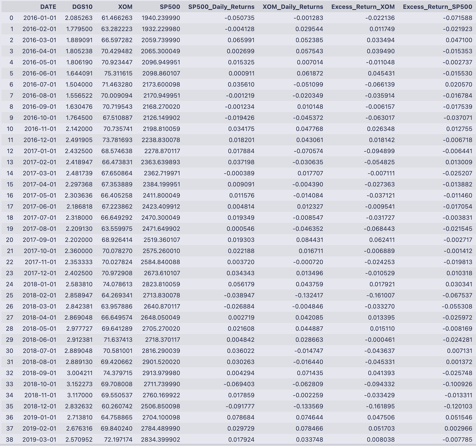

The two assignment lines add excess-return columns to Mdata by subtracting the risk-free rate from each asset return. The first line creates a column named “Excess_Return_<tick>” (whatever string tick holds) by taking the column “<tick>_Daily_Returns” and subtracting Mdata[‘DGS10’].astype(‘float’) / 100. The second line does the same for the S&P column, creating “Excess_Return_SP500” from “SP500_Daily_Returns” minus the same DGS10/100 term.

- Mdata[‘DGS10’].astype(‘float’) / 100 converts the DGS10 values (which may be stored as strings) into numeric decimals. Dividing by 100 turns a percentage-like value (e.g., 2.085263) into a decimal rate (0.02085263) so it can be subtracted from the return series that are already in decimal form (e.g., -0.001283).

- The subtraction is done elementwise for each row, so each excess return corresponds to the same date/row in Mdata.

- The column name for the asset excess return is dynamically created with format(tick), so if tick == ‘XOM’ the new column is “Excess_Return_XOM”.

The printed DataFrame shows those new columns appended on the right. For example, on 2016–01–01 DGS10 = 2.085263, XOM_Daily_Returns = -0.001283, and SP500_Daily_Returns = -0.050735. The code computed:

- Excess_Return_XOM = -0.001283–0.02085263 ≈ -0.022136

- Excess_Return_SP500 = -0.050735–0.02085263 ≈ -0.071588

You can see that pattern throughout the table: each asset return has the numeric DGS10/100 subtracted, so when the risk-free rate is positive the excess return is more negative than the raw return, and when the asset return is strongly positive the excess return remains positive after the subtraction. The columns line up by date and show these computed excess returns for every row printed.

# Running a regression to calculate Beta
# Can play around with what risk free rate to use to get your relative beta.
results = smf.ols(’Excess_Return_{} ~ Excess_Return_SP500’.format(tick), data = Mdata).fit()

This line builds and fits a linear regression that estimates how the series named “Excess_Return_<tick>” moves with “Excess_Return_SP500”.

A few moving parts, in plain terms:

- The string ‘Excess_Return_{} ~ Excess_Return_SP500’.format(tick) produces a formula text like “Excess_Return_XOM ~ Excess_Return_SP500” (if tick is “XOM”). In the statsmodels formula language the left side of ~ is the dependent variable and the right side is the independent variable.

- smf.ols(…, data = Mdata) tells statsmodels to create an Ordinary Least Squares model object using that formula, looking up the variable names as columns inside the DataFrame Mdata.

- .fit() actually runs the estimation and returns a fitted model object, which is stored in the variable results.

So after this line executes, results holds the fitted regression (it contains the intercept and the slope coefficient — the slope on Excess_Return_SP500 is the estimated beta you’re after). This assignment by itself doesn’t print anything; you can inspect the outcome with methods like results.summary() to see the regression table, results.params to read coefficients (e.g., results.params[‘Excess_Return_SP500’] for the beta), or results.predict(…) to get fitted values.

Note that this is a standard OLS setup: it assumes a linear relation between the excess returns and that the usual OLS assumptions about the residuals hold if you want to interpret inference (standard errors, p-values) in the usual way.

print(results.summary())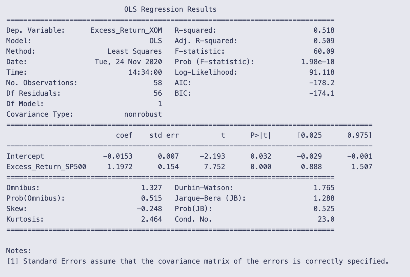

You’re printing the text summary that statsmodels produces for a fitted OLS regression object. That summary collects the model metadata, goodness-of-fit statistics, the coefficient table, and several diagnostic tests in a compact, human-readable table.

Looking at the top area, you can see the dependent variable name (Excess_Return_XOM), the model type (OLS), number of observations (58), R-squared (0.518) and adjusted R-squared (0.509). R-squared ≈ 0.518 means the single predictor explains about 51.8% of the variation in the dependent variable. The F-statistic (60.09) and its tiny p-value (1.98e-10) tell you the model as a whole is statistically significant.

The coefficient table gives the intercept and the slope on Excess_Return_SP500 with standard errors, t-stats, p-values, and 95% confidence intervals. Concretely:

- Intercept = -0.0153, std err 0.007, t = -2.193, p = 0.032, 95% CI ≈ [-0.029, -0.001]. In the units used for the regression, the intercept is negative and statistically different from zero at the 5% level (if returns are in fractions, -0.0153 ≈ -1.53%).

- Excess_Return_SP500 coefficient = 1.1972, std err 0.154, t = 7.752, p ≈ 0.000, 95% CI ≈ [0.888, 1.507]. That slope is large and highly significant, and its confidence interval does not include zero, so the predictor has a robust positive association with the dependent variable.

The lower part shows diagnostic statistics. Durbin–Watson = 1.765 is reasonably close to 2 (which would indicate no autocorrelation), so there’s no strong evidence of problematic serial correlation. Omnibus and Jarque–Bera tests have p-values well above 0.05, and skew/kurtosis values are near normal, so there’s no strong evidence the residuals deviate from normality. The condition number (23.0) is small, so numerical conditioning or multicollinearity isn’t a concern here (also expected with only one predictor).

Finally, note the “nonrobust” covariance type: the standard errors, t-stats and p-values assume the usual OLS assumptions (homoscedastic, independent errors). If you suspect heteroscedasticity or serial correlation, you’d compute robust or clustered standard errors before relying on the p-values.

# Beta from the OLS above
Beta = 1.0775
# Once we have Beta, we can calculate the expected return of the company BASED on the market.
average_risk_free_rate = Mdata[’DGS10’].astype(’float’).mean() /100
# Using the Historical Rate of return for the S&P500 market...
# Including dividends but not accounting for inflation
average_return_SP500 = (1.311 * (1-.0441) * (1.2194) * (1.1193) * (1.0131) * (1.1381))**(1/5) - 1

print(’Average Risk Free Rate’,average_risk_free_rate)
print(’Average Return S&P500’,average_return_SP500)
print(’Expected Return of {}’.format(tick),average_risk_free_rate + Beta * (average_return_SP500 - average_risk_free_rate))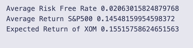

You set Beta to 1.0775 (the comment says it came from the OLS above, so it’s being used as the company’s sensitivity to market moves) and then compute an expected return using the standard CAPM structure: expected_return = risk_free_rate + Beta * (market_return — risk_free_rate).

- average_risk_free_rate is taken from Mdata[‘DGS10’].astype(‘float’).mean() / 100. That converts whatever values are stored in Mdata[‘DGS10’] to floats, averages them, and divides by 100 to move from percentage points into decimal form (so 2.06% becomes 0.0206).

- average_return_SP500 is computed as (1.311 * (1-.0441) * 1.2194 * 1.1193 * 1.0131 * 1.1381)**(1/5) — 1. In words: multiply a sequence of growth factors together, take the fifth root (which annualizes the five-year cumulative growth), then subtract one to turn the annualized growth factor into an annual return in decimal form. That gives the assumed average annual S&P 500 return used here.

- The final printed expected return uses the formatted tick variable in the label, so it prints “Expected Return of XOM” followed by the calculated decimal return.

- Average Risk Free Rate: 0.02063015824879768 (about 2.063%).

- Average Return S&P500: 0.14548159954598372 (about 14.55%).

- Expected Return of XOM: 0.15515758624651563 (about 15.52%).

If you break down the CAPM arithmetic behind that last number:

- Market risk premium = average_return_SP500 — average_risk_free_rate = 0.1454816–0.02063016 ≈ 0.12485144.

- Beta × market premium = 1.0775 × 0.12485144 ≈ 0.13452743.

- Add the risk-free rate: 0.02063016 + 0.13452743 ≈ 0.15515759, which matches the printed expected return.

So the cell takes the chosen Beta, an average treasury rate (converted to decimal), and an annualized S&P500 return (computed from the product of provided factors), and applies the CAPM formula to produce an expected annual return for the ticker named by tick (XOM in this run).

Download entire source code using the button below: