Quantitative Trading Model from Paper to Python: Building an Attention-BiLSTM Strategy for Gold and Bitcoin

A step-by-step tutorial on translating academic paper concepts—including temporal attention, streak-based position sizing, and greedy portfolio optimization—into production-ready Python code.

What This Article Builds

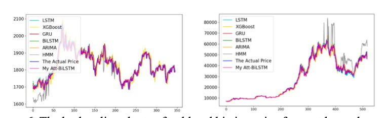
The paper proposes a quantitative trading pipeline for gold and Bitcoin. It combines price forecasting with an attention-enhanced bidirectional LSTM, position sizing based on empirical consecutive rises and declines, transaction-cost sensitivity analysis, and claimed use of VaR and a modified greedy algorithm for trading decisions. Several benchmark forecasting models are compared, with Att-BiLSTM reported as the best predictor. The trading results claim a final value of approximately $646 for a $500 gold allocation and $215,487 for a $500 Bitcoin allocation, although the backtest protocol and several model details are insufficiently specified.

---

The code is my implementation based on what the paper discusses. Download the source code using the button at the end of this article!

Also the code might have some errors, because I didn’t found anything online related to paper, everything is implemented by myself, so download it and understand. With article and the code.

This is the research paper I tried to implement: https://www.researchgate.net/publication/364569615_Research_on_Quantitative_Trading_Model

Our Book is out on openclaw:

---

Implementation Assumptions

• Historical gold and Bitcoin datasets are not supplied; the implementation will accept local CSV or pandas DataFrame inputs and include a deterministic synthetic-data generator for demonstrations only.

• Prices are assumed to be positive, chronologically ordered observations with one row per asset and an explicit timestamp.

• Standard simple return, (pt-p{t-1})/p_{t-1}, is used by default because the paper's printed denominator is ambiguous; the choice is configurable and documented.

• The primary target is a one-step-ahead normalized price or return forecast. A three-step vector forecast option is supported because the paper's conclusion mentions three-day forecasts.

• The primary forecasting model is an attention-enhanced BiLSTM with a configurable learned query vector, 20% dropout, MAE loss, and RMSprop optimizer.

• The paper-style 70:30 chronological split is supported for comparison, while walk-forward evaluation is the preferred protocol for trading conclusions.

• Equations (5) through (8), VaR operation, and the modified greedy algorithm are implemented as explicit reconstructions and will never be presented as exact reproductions.

• Transaction fees apply to both buys and sells by default, use decimal rates such as 0.002 for 0.2%, and are configurable.

• The backtest uses next-bar execution after a signal, finite position-addition levels, no leverage by default, and optional slippage.

• The reported final values of approximately 646 USD for gold and 215487 USD for Bitcoin are recorded as unverified reference claims rather than expected test outputs.

• Deep-learning, statistical, and optional benchmark dependencies are isolated so core data, sizing, risk, and backtesting components remain usable without every optional package installed.

1. The Paper’s Core Idea: Forecast Timing and Manage Position Size Separately

The paper is trying to answer two different trading questions:

When should the strategy trade?

How much capital should it deploy when it trades?

Those questions are related, but they are not the same problem. A forecasting model can estimate that gold or Bitcoin may rise, yet it does not automatically determine whether the strategy should invest $10, $100, or the entire available budget. Conversely, a position-sizing rule can specify how much to buy after a decline, but it needs a signal to decide whether buying is appropriate at that moment.

The implementation keeps these responsibilities separate. The forecasting component produces information about a possible future price. The signal layer converts that forecast into a buy, sell, add, or hold decision. The sizing layer proposes an amount. Risk control can reject or reduce that amount. Finally, the execution and accounting layer applies transaction costs, updates cash and holdings, and measures the resulting portfolio.

This separation is especially important because several parts of the paper are incompletely specified. The paper gives a broad design involving an attention-enhanced BiLSTM, consecutive-rise and decline analysis, exponential position sizing, VaR, and a modified greedy algorithm. It does not fully define every interface between those components. A modular Python implementation makes each interpretation visible instead of hiding assumptions inside one large trading function.

The complete data-to-portfolio flow

The project’s README presents the intended architecture as a pipeline:

local prices
    -> cleaning and chronological split
    -> leakage-safe sliding windows
    -> forecast model
    -> buy / sell / hold signal
    -> finite exponential position-size schedule
    -> historical VaR filter
    -> reconstructed greedy action selection
    -> next-bar execution with fees and slippage
    -> portfolio valuation and performance metrics

Each stage has a distinct responsibility:

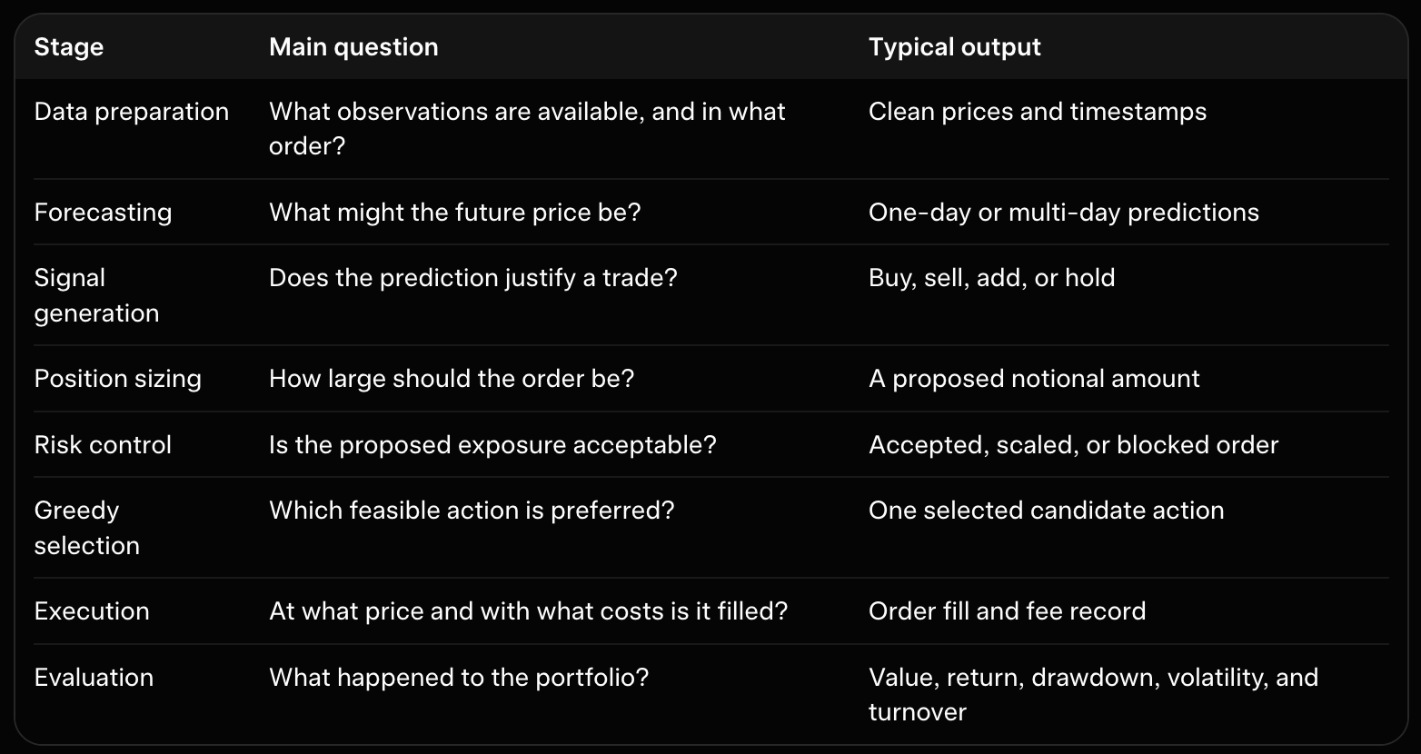
The paper’s primary model is the attention-enhanced BiLSTM, or Att-BiLSTM. It processes a historical sequence and uses temporal attention to produce a representation for forecasting. The input sequence is built from a sliding window, reported as 100 observations with stride one. The resulting prediction is not itself a trade: it must be aligned with a timestamp and passed to a decision policy.

The position-management component is conceptually independent of the neural network. It analyzes gains and declines, estimates statistics such as representative gain and decline magnitudes, and uses an exponential schedule to increase later additions. Because the paper’s position-sizing equations are corrupted or incomplete in the extracted source, the Python project treats this as a documented normalized exponential reconstruction rather than an exact transcription.

Why the boundaries matter

A single function that loads prices, trains a model, decides an order, and reports profit would be difficult to audit. It would also make it unclear whether future information entered the decision process. The generated package instead plans separate modules for data, models, streak analysis, sizing, risk, strategy, and backtesting.

For example, DataConfig makes the forecasting window explicit:

@dataclass
class DataConfig:
    """Configuration for local historical-price preparation."""

    timestamp_column: str = "timestamp"
    price_column: str = "price"
    asset_column: Optional[str] = None
    window_length: int = 100
    stride: int = 1
    return_definition: str = "simple"
    zero_return_policy: str = "break"

The values window_length=100 and stride=1 reflect the paper’s stated sliding-window setup. Other fields expose choices that the paper does not settle, such as how returns are defined and how zero returns affect streaks. Making these values configuration fields means a later experiment can record exactly which interpretation it used.

The data layer represents a cleaned asset as PriceData, a small object containing timestamps, prices, and an asset label. Its validation contract requires unique, increasing timestamps and finite positive prices. That contract is more than cosmetic. A negative or missing price can invalidate returns, position sizes, portfolio valuation, and risk calculations downstream.

The WindowedDataset object preserves temporal metadata in addition to arrays:

@dataclass(frozen=True)
class WindowedDataset:
    """Windowed samples and their temporal metadata."""

    X: np.ndarray
    y: np.ndarray
    window_start: pd.DatetimeIndex
    window_end: pd.DatetimeIndex
    y_timestamp: pd.DatetimeIndex
    feature_names: Tuple[str, ...] = ("price",)

Keeping window_end and y_timestamp is important. A model prediction must be associated with the time at which its input information became available. The later backtest can then enforce the rule that a signal generated after the final input observation cannot fill at an earlier or identical timestamp.

Separating a forecast from an order

The paper’s forecasting section and trading section imply different horizons. The prediction tables appear to use a one-step setup, while the conclusion refers to forecasts for the next three days. The implementation therefore exposes the forecast horizon rather than assuming that those descriptions are identical.

Conceptually, a one-step window is:

\[ Xt = [z{t-99}, z{t-98}, \ldots, zt], \qquad yt = z{t+1}. \]

A three-step version is:

\[ yt = [z{t+1}, z{t+2}, z{t+3}]. \]

The forecast layer answers what the model predicts. A separate signal layer must decide how to interpret that prediction. For example, it might compare the terminal three-day forecast with the current price, or use a configured threshold before producing a buy signal. That rule is a strategy assumption, not a consequence of the neural network itself.

The same distinction applies to sizing. A positive forecast does not imply that the strategy should invest its full available balance. The sizing schedule may allocate one of several finite addition levels, subject to cash and exposure caps. The eventual order amount is therefore the result of several stages:

forecast
    -> directional signal
    -> candidate order amount
    -> risk adjustment
    -> selected feasible action
    -> executed fill

This decomposition also makes it possible to compare alternatives. The same forecast can be evaluated with a flat allocation, the reconstructed exponential schedule, or a different risk limit. Likewise, the same sizing rule can be tested with Att-BiLSTM predictions or a simpler benchmark.

Offline and educational by design

The generated project is deliberately offline. It accepts local CSV files or deterministic synthetic data and does not connect to an exchange, download market data, handle credentials, or submit orders. This restriction is appropriate for a paper-to-code tutorial because it keeps the focus on data alignment, modeling assumptions, decision rules, and accounting.

Synthetic data are useful for demonstrating interfaces. For example, the data module includes a deterministic generator whose purpose is to provide repeatable price paths for checking window shapes and portfolio arithmetic. Such data are not evidence about gold or Bitcoin and cannot reproduce the paper’s reported outcomes.

The package initializer reinforces this design by avoiding model training or data loading during import:

"""Offline research components for the quantitative trading model paper."""

# Configuration is part of the lightweight public API. Heavy forecasting and
# benchmark dependencies are imported only by their respective modules.
from .config import (
    BacktestConfig,
    DataConfig,
    ExecutionConfig,
    FeeSensitivityConfig,
    ForecastConfig,
    SizingConfig,
    SplitConfig,
    VaRConfig,
    validate_config,
)

This side-effect-free structure lets a reader use data preparation, streak analysis, sizing, risk, or accounting utilities without installing PyTorch or every optional benchmark library. It also avoids implying that importing the package performs a market action.

What this architecture does—and does not—claim

The architecture provides a practical way to translate the paper’s major ideas into independently inspectable components. It directly reflects the clearly described mechanics, such as sliding windows and temporal attention, while making incomplete parts configurable and labeled as reconstructions.

It does not establish that the paper’s strategy is profitable or that the implementation reproduces its reported numbers. The paper’s approximate final values—$646 from a $500 gold allocation and $215,487 from a $500 Bitcoin allocation—remain unverified claims because the original data, dates, execution rules, risk settings, and position-sizing details are unavailable.

The useful starting point is therefore not a promise of matching those numbers. It is a disciplined contract between modules:

• data provides only ordered historical observations;

• forecasting uses a defined historical window;

• signals use predictions and current state;

• sizing uses a finite, explicit budget;

• risk control uses pre-decision information;

• execution occurs after the signal timestamp;

• evaluation accounts for costs and reports portfolio behavior separately from forecast error.

That contract is the foundation for the remaining sections, where each component is examined in detail and every reconstruction decision is identified.

2. What Can Actually Be Reproduced?

The paper separates two decisions: forecasting proposes when a trade might be useful, while position management proposes how much capital to deploy. Before implementing those components, distinguish a direct implementation from a reconstruction or an illustrative example.

A paper-to-code project can contain clean Python and still fail to reproduce the original experiment. Reproduction requires the same data, timestamps, preprocessing, model definition, decision rules, execution assumptions, and evaluation protocol. Several of those ingredients are missing or ambiguous here.

The project uses five status labels, consistent with docs/reproduction_matrix.md:

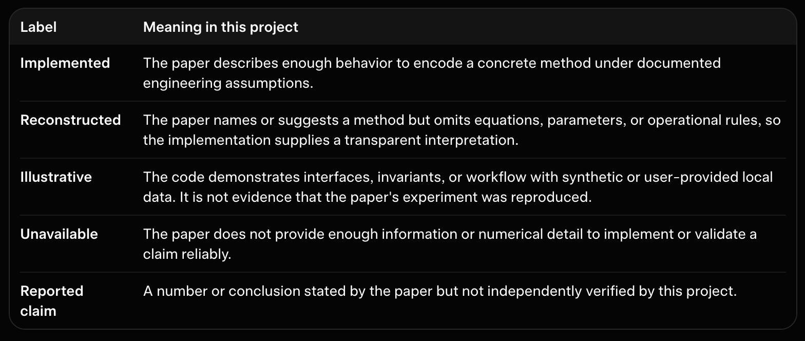
These labels determine how results should be interpreted and whether a value may legitimately be used as a test expectation. A hand-calculated fee or accounting invariant can be tested. The paper's final portfolio values cannot be treated that way because their inputs and protocol are unknown.

2.1 What the paper specifies clearly

Several elements are concrete enough to guide implementation:

• overlapping historical windows of length 100 with stride 1;

• an attention-enhanced bidirectional LSTM as the primary forecasting model;

• comparisons with LSTM, GRU, BiLSTM, Holt-Winters, ARIMA, HMM, and XGBoost;

• a stated dropout setting of 20%;

• MAE as the training loss;

• RMSprop as the intended optimizer after correcting the paper's terminology;

• dot-product attention, softmax normalization, and a weighted temporal sum;

• transaction-fee scenarios for gold and Bitcoin.

For example, src/quantitative_trading_model/models/attention.py can implement the displayed attention equations without knowing the authors' complete source code. Similarly, the configuration modules can preserve paper-inspired values as visible settings. This still does not guarantee numerical reproduction: the data, model dimensions, initialization, and training schedule remain unknown.

Configuration provenance is deliberately split across modules rather than concentrated in ForecastConfig:

• DataConfig contains the window length, stride, cleaning, and data conventions;

• ForecastConfig contains model and training settings such as horizon, dropout, loss, optimizer, and hidden dimensions;

• SizingConfig contains the reconstructed position-sizing settings;

• VaRConfig contains risk-estimation and action settings;

• ExecutionConfig and BacktestConfig contain fees, slippage, cash, leverage, and liquidation assumptions;

• FeeSensitivityConfig contains the gold and Bitcoin fee grids.

This separation prevents unrelated assumptions from being hidden behind a misleading single model configuration.

2.2 Missing data and experiment identity

The largest reproducibility gap is the input data. The paper refers to historical gold and Bitcoin prices but does not identify enough information to establish exactly what those series represent. Missing details include:

• the data vendor or source;

• the specific gold instrument and Bitcoin market or index;

• currency and unit conventions;

• sampling frequency;

• start and end dates;

• timezone and timestamp rules;

• the selected price field, such as close or adjusted close;

• treatment of missing observations and duplicate timestamps;

• market closures, splits, or other instrument-specific adjustments;

• whether the assets were processed independently or jointly.

“Gold price” and “Bitcoin price” are not unique datasets. Two valid historical series can have different timestamps, gaps, price fields, and price levels. A model trained on either series may be reasonable while producing metrics that cannot be compared with the paper's table.

README.md, data.py, and cli.py therefore require local inputs rather than silently selecting an unidentified market-data source. Synthetic data are available only for demonstrations. This makes provenance explicit and avoids implying that an arbitrary local or synthetic series is equivalent to the paper's input.

2.3 Missing preprocessing and target definition

The paper does not fully state what the forecasting model predicts. Plausible interpretations include:

a raw next-day price;

a normalized price level;

a one-day return or percentage change;

a vector of the next three prices;

a day-three price produced by a multi-step procedure.

The prediction discussion is compatible with one-step forecasting, while the conclusion refers to forecasts over the next three days. These are different supervised-learning problems with different target shapes, losses, inverse transformations, and trading signals.

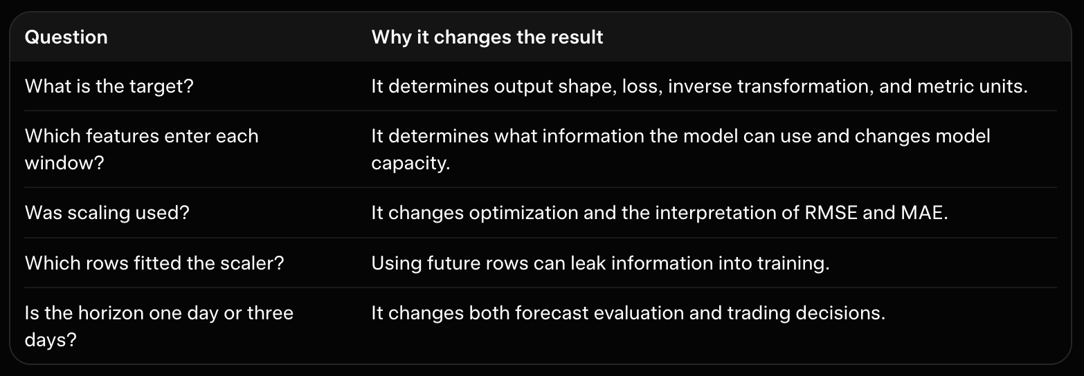
Preprocessing is also unclear. The paper does not specify whether prices were scaled, whether scaling used training observations only, or whether features such as volume, technical indicators, or macroeconomic variables were included. The implementation defaults to a price-based setup but exposes the target representation and horizon so that this ambiguity remains visible.

A reproduction must record at least:

2.4 Missing Att-BiLSTM architecture details

Att-BiLSTM identifies a model family, not a complete architecture. The paper does not reliably specify:

• the number of recurrent layers;

• hidden-state dimensions;

• whether attention receives concatenated forward and backward states;

• how the query vector is constructed;

• dense-layer dimensions and activations;

• output shape and activation;

• recurrent versus ordinary dropout;

• initialization;

• learning-rate and optimizer settings;

• batch size, epoch count, and stopping rule;

• random seed;

• whether each asset receives a separate model.

models/forecasters.py consequently provides a configurable paper-inspired model. Its learned attention query is an explicit reconstruction: the paper supplies a symbol q but does not say how that vector is obtained. The implementation is useful and inspectable, but it is not a verified transcription of the authors' architecture.

The same caution applies to the benchmarks. Listing LSTM, GRU, BiLSTM, Holt-Winters, ARIMA, HMM, and XGBoost does not establish that their feature sets, capacities, tuning procedures, and horizons were comparable. The paper's statement about “consistent parameters” is insufficient to reconstruct a fair benchmark protocol.

2.5 The position-sizing equations are incomplete

Equations (5) through (8) in the position-management section are not reliably recoverable from the extracted material. Important ambiguities include:

• whether p_i denotes cash, asset units, or notional exposure;

• the meaning of the maximum addition count x;

• whether fees apply to one transaction or both sides;

• whether decline statistics are signed or expressed as positive loss magnitudes;

• the independent variable in the exponential expression;

• whether additions follow every decline or only a forecast-confirmed condition.

src/quantitative_trading_model/sizing.py therefore does not claim to transcribe the equations. It implements a normalized exponential schedule with finite addition levels, cash limits, and exposure caps. This is a reconstructed exponential position-sizing rule: it captures the apparent idea that later additions receive larger weights, but it does not establish that the paper used the same formula or calibration.

Keeping this reconstruction in one module is useful. If the original equation images or source become available, the sizing implementation can be replaced without changing data preparation, forecasting, risk, or portfolio accounting.

2.6 VaR is named but not operationally defined

The paper says that VaR contributes to trading decisions but does not supply the settings needed for a unique procedure. Missing choices include:

• confidence level;

• horizon;

• estimation-window length;

• historical, parametric, or Monte Carlo method;

• portfolio-level versus asset-level returns;

• treatment of overlapping multi-day returns;

• maximum acceptable loss;

• whether VaR blocks, scales, or merely reports a trade.

src/quantitative_trading_model/risk.py provides a rolling historical VaR reconstruction with explicit confidence, lookback, horizon, and action settings. It supports leakage-aware use, but it cannot independently guarantee temporal provenance: HistoricalVaR accepts caller-provided returns and does not infer timestamps. The surrounding caller or backtest must supply only returns known before the decision and must exclude the current or future return when appropriate.

Thus, a VaR value means “the result of this configured historical quantile on this supplied return window.” It is not a hidden setting recovered from the paper, and it should not be described as the paper's exact VaR method.

2.7 The modified greedy algorithm is not reproducible from its name

“Modified greedy algorithm” describes a family of procedures, not one precise policy. Reproduction would require the paper to define:

• candidate actions;

• whether actions are buy, sell, hold, or additions;

• the objective being maximized;

• how forecasts become expected gains;

• how fees enter the objective;

• cash, exposure, and addition constraints;

• how VaR affects feasibility;

• whether one action or a multi-step plan is selected;

• tie-breaking behavior.

src/quantitative_trading_model/strategy.py implements a transparent reconstruction: enumerate feasible candidates, estimate forecast-based benefit after fees, apply documented constraints, and select the highest-scoring candidate with deterministic tie-breaking. It must not be described as the paper's verified algorithm.

There is also an unresolved static integration issue. The generated GreedyPolicy adapter currently does not match the generated VaRTradeFilter interface: it attempts to pass proposed_notional and omits required exposure-related arguments, while the filter expects proposed_quantity together with current exposure and portfolio value. This boundary must be repaired before runtime integration is attempted. Until then, the strategy and risk modules should be treated as separately documented reconstructions rather than a verified end-to-end combination.

The temporal rule remains essential: realized future returns must never score a candidate. A decision may use forecasts, current cash, current holdings, current exposure, and pre-decision risk history, but not the price that will be observed after execution.

2.8 Why the headline profits are not test targets

The paper reports approximately:

• $646 from an initial $500 gold allocation;

• $215,487 from an initial $500 Bitcoin allocation;

• approximately $216,133 from the combined $1,000 allocation.

These are reported claims, not reproduced results. src/quantitative_trading_model/experiments.py records the values as unverified references rather than using them as test assertions or expected outputs from synthetic demonstrations.

A test target is appropriate when its input and protocol are specified. For example, a hand-calculated accounting test can assert the cash effect of a purchase with a known fee. The paper's Bitcoin figure cannot be tested this way because the historical period, asset series, signal timestamps, sizing triggers, reinvestment rules, exposure limits, fee convention, slippage, and liquidation policy are unknown.

A local result that happens to resemble one of those values would not prove reproduction unless the underlying data and all decision and accounting rules also matched. The unusually large Bitcoin result may depend on a particular historical period, aggressive compounding, repeated averaging down, leverage-like exposure, or optimistic execution assumptions. It should not be generalized as evidence of future profitability.

2.9 Benchmark metrics and fee figures are also unverified

The paper reports forecast metrics such as RMSE, MAE, MAPE, and R-squared, and shows transaction-fee sensitivity figures. Those values cannot be confirmed from the extracted text alone.

Forecast metrics depend on the exact test observations, target scale, transformations, timestamps, MAPE zero policy, architecture, trained parameters, random seed, and stopping rule. Fee figures additionally depend on trade dates and quantities, fee side conventions, spread, slippage, action feasibility, initial holdings, reinvestment, and liquidation.

The implementation preserves the paper-inspired fee grids as inputs: gold rates from 0.2% through 1.2%, and Bitcoin rates from 1.5% through 3.5%. It cannot infer the missing y-values from the figures. A new fee sweep using identified local data is a valid experiment under the project's assumptions, not a recovered copy of the paper's chart.

2.10 How to read the reproduction matrix

docs/reproduction_matrix.md records status at the method and claim level. Its distinctions are important:

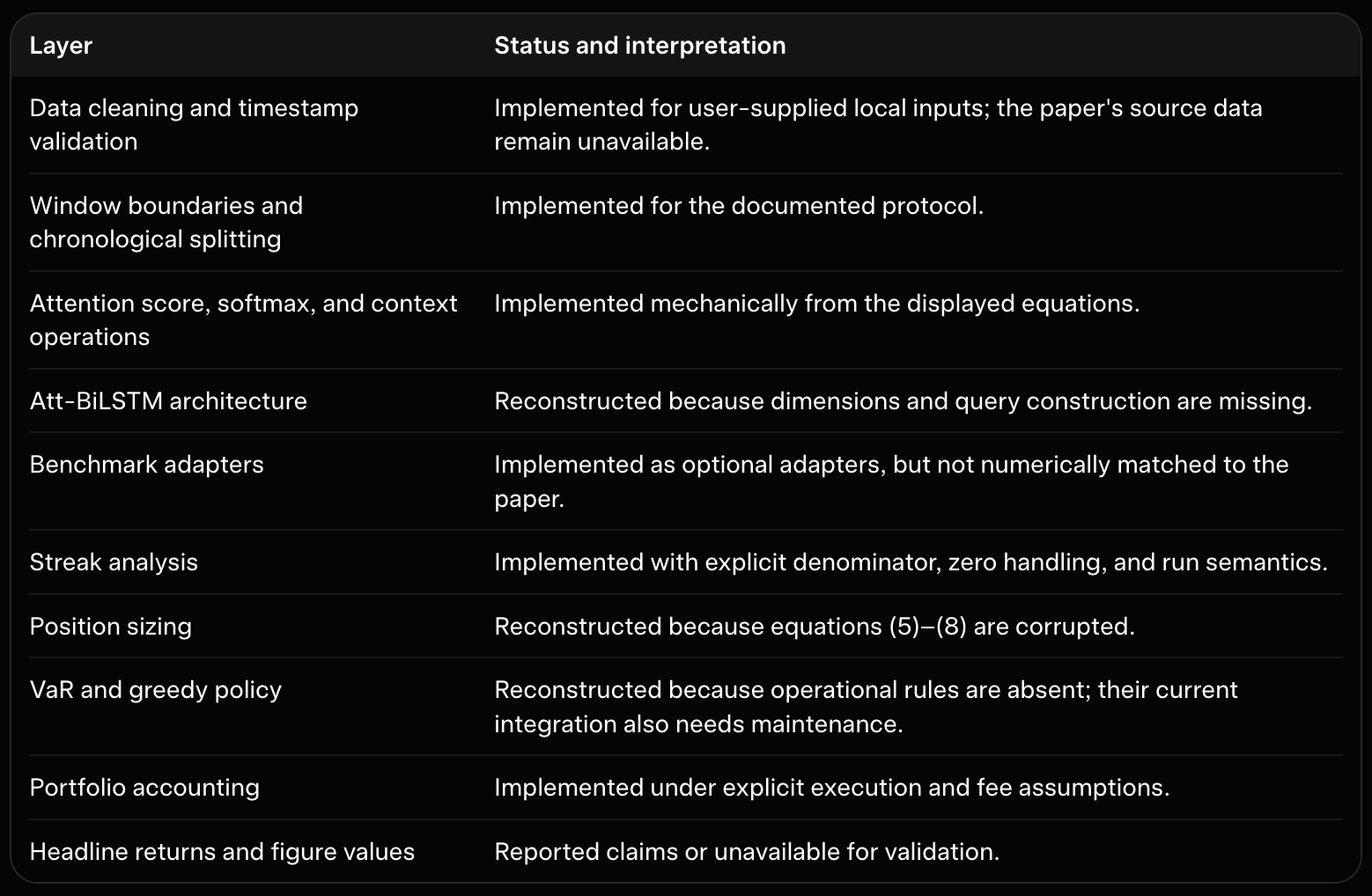
This matrix prevents every function from being presented with the same level of authority when some functions implement displayed equations and others embody missing decisions.

2.11 Static review is not empirical reproduction

The project raises two different verification questions:

Does the generated artifact appear structurally reviewable?

Does the implementation reproduce the paper's empirical behavior?

Static and semantic review can address parts of the first question. It can inspect Python parsing, expected symbols, configuration validation, tensor-shape contracts, attention normalization, temporal boundaries, budget invariants, and accounting formulas. It cannot establish that the paper's data, model, or financial results were reproduced.

The supplied local verification record did not pass completely. It reported placeholder-detection findings for experiments.py and cli.py, and Markdown-fence findings for the generated README.md and docs/tutorial.md code fields. These are generated-artifact quality findings. They are not runtime results and do not by themselves demonstrate a Python syntax failure or a financial-model failure.

Semantic code verification was skipped. Runtime execution and test-suite success therefore must not be claimed. In addition, some generated tests and orchestration functions appear to use APIs that are not fully aligned with the generated modules, including the strategy/VaR boundary described above. Those inconsistencies require a software-maintenance pass before execution is attempted.

The appropriate conclusion is limited: the project documents intended interfaces, assumptions, and invariants, but it is not an executed or empirically validated reproduction.

2.12 Responsible interpretation policy

When describing results from this project:

• say implemented for mechanics supported by the paper and the code contract;

• say reconstructed for normalized sizing, historical VaR, the greedy policy, and other interpretations of missing details;

• say illustrative for synthetic data and hand-calculated workflows;

• say unavailable when the source lacks the information needed for implementation or validation;

• say reported claim when quoting the paper's profits or metrics without independent validation;

• do not call a run on a different local dataset an exact reproduction;

• keep forecast metrics separate from portfolio metrics;

• report dates, data provenance, target definition, fees, slippage, turnover, drawdown, and liquidation rules with every backtest;

• treat static review as artifact evidence, not proof of execution, profitability, or paper fidelity.

The next sections can discuss setup and implementation without blurring these categories. A modular reconstruction can still teach attention-based forecasting, streak statistics, bounded sizing, risk filtering, and fee-aware accounting while making clear which conclusions require the original data and experimental protocol.

3. Project Setup and the Implementation Map

The implementation is organized as a normal Python package rather than as one large research script. That choice matters because the paper combines several different responsibilities: data preparation, neural forecasting, benchmark models, streak analysis, position sizing, risk filtering, trading decisions, execution, and evaluation. Keeping those responsibilities in separate modules makes it easier to inspect assumptions and replace incomplete reconstructions later.

The project is also deliberately offline. It accepts local files or generated demonstration data, but it does not connect to an exchange, download market data, store credentials, or submit orders. The resulting code is suitable for educational research and backtest prototyping, not for live trading.

3.1 The src layout

The package uses the conventional src layout:

quantitative-trading-model/
├── pyproject.toml
├── README.md
├── src/
│   └── quantitative_trading_model/
│       ├── __init__.py
│       ├── config.py
│       ├── data.py
│       ├── metrics.py
│       ├── streaks.py
│       ├── sizing.py
│       ├── risk.py
│       ├── strategy.py
│       ├── backtest.py
│       ├── experiments.py
│       ├── cli.py
│       └── models/
│           ├── attention.py
│           ├── forecasters.py
│           └── benchmarks.py
├── tests/
└── docs/
    ├── tutorial.md
    └── reproduction_matrix.md

With this layout, the importable package lives under src/quantitative_trading_model, while documentation and tests remain outside the runtime package. The pyproject.toml file tells setuptools where to find the package:

[tool.setuptools]
package-dir = { "" = "src" }
include-package-data = true

[tool.setuptools.packages.find]
where = ["src"]

This avoids a common development problem in which tests accidentally import a loose source directory instead of the package that users will install. It also gives the project a clear boundary: files under src/quantitative_trading_model are implementation modules, while the root-level documentation explains how to use and interpret them.

3.2 Core dependencies and optional model dependencies

The package keeps its required dependencies small:

[project]
requires-python = ">=3.10"
dependencies = [
    "numpy>=1.24",
    "pandas>=2.0"
]

NumPy and pandas support the parts of the project that do not require a deep-learning framework: local price tables, timestamp handling, return calculations, streak statistics, metrics, risk calculations, and portfolio accounting.

The heavier forecasting libraries are optional:

[project.optional-dependencies]
deep-learning = [
    "torch>=2.0"
]
classical = [
    "statsmodels>=0.14",
    "pmdarima>=2.0",
    "hmmlearn>=0.3",
    "xgboost>=2.0"
]

This split reflects the paper's structure. The Att-BiLSTM requires PyTorch, but a reader who only wants to study the return convention, normalized exponential sizing reconstruction, historical VaR, or portfolio accounting should not need to install PyTorch. Similarly, Holt-Winters, ARIMA, HMM, and XGBoost benchmarks can be enabled only when those comparisons are needed.

The optional dependency design also makes missing capabilities visible. A benchmark adapter should report that a library is unavailable rather than silently substituting a different model. That distinction matters when comparing results with the paper: an omitted benchmark is not the same as a benchmark that produced a poor score.

The package metadata also defines a console entry point:

[project.scripts]
quant-trading-model = "quantitative_trading_model.cli:main"

After local installation, this exposes the offline command-line interface as quant-trading-model. The CLI can validate local CSV files, generate deterministic synthetic demonstrations, and dispatch configured research experiments. It does not create a network client or read credentials.

3.3 Side-effect-free package imports

The package initializer intentionally exposes only lightweight metadata and configuration types:

"""Offline research components for the quantitative trading model paper."""

from importlib import metadata

try:
    __version__ = metadata.version("quantitative-trading-model")
except metadata.PackageNotFoundError:
    __version__ = "0.1.0"

from .config import (
    BacktestConfig,
    DataConfig,
    ExecutionConfig,
    FeeSensitivityConfig,
    ForecastConfig,
    SizingConfig,
    SplitConfig,
    VaRConfig,
    validate_config,
)

Importing the package does not load a CSV, train a model, create a portfolio, or contact an external service. The initializer also does not import PyTorch, statsmodels, hmmlearn, or XGBoost. Those imports are deferred to the modules that need them.

That design has two practical benefits:

Lightweight use: core modules remain usable in an environment without optional modeling libraries.

Predictable imports: simply writing import quantitative_trading_model cannot start a computation or produce an external side effect.

The public exports are deliberately narrow:

__all__ = [
    "__version__",
    "BacktestConfig",
    "DataConfig",
    "ExecutionConfig",
    "FeeSensitivityConfig",
    "ForecastConfig",
    "SizingConfig",
    "SplitConfig",
    "VaRConfig",
    "validate_config",
]

The model, data, strategy, and backtest classes are imported from their own modules when required. This keeps the top-level API stable without forcing every user to install every optional dependency.

3.4 Where each research responsibility lives

The package map follows the paper's conceptual pipeline:

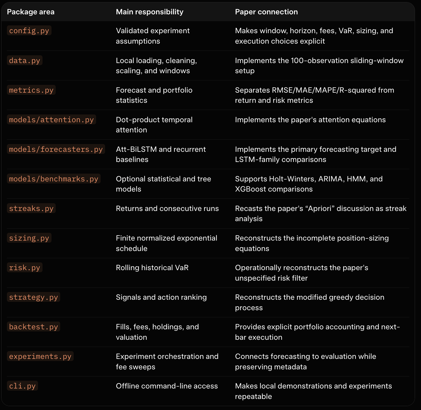
This separation is not merely a software-style preference. It prevents an ambiguous paper detail from being hidden inside an unrelated function. For example, the return denominator belongs in streaks.py, while the execution fee convention belongs in backtest.py. A reader can therefore change one assumption without accidentally changing every layer of the research pipeline.

3.5 Documentation, tests, and the reproduction matrix

The non-runtime files serve different purposes:

• `README.md` gives installation instructions, local CSV conventions, CLI examples, project warnings, and a high-level architecture map.

• `docs/tutorial.md` explains the paper-to-code translation in detail, including equations, tensor shapes, timing rules, and reconstruction decisions.

• `docs/reproduction_matrix.md` tracks each paper component as implemented, reconstructed, illustrative, unavailable, or an unverified reported claim.

• `tests/` contains hand-calculable checks for data boundaries, streak semantics, sizing budgets, VaR decisions, model shapes, transaction fees, and portfolio-value identity.

The reproduction matrix is especially useful for this paper because the source does not fully specify equations (5)–(8), VaR operation, the greedy policy, or the original backtest protocol. Instead of allowing those gaps to disappear into code, the matrix records what the implementation can support and what still requires the original data or source material.

For example, the matrix treats the following differently:

• the 100-step window as a directly implementable paper detail;

• the learned attention query as a reconstruction;

• synthetic prices as an illustration;

• the reported $646 gold and $215,487 Bitcoin outcomes as unverified claims.

That classification should remain visible in experiment output and documentation. A clean package installation does not establish empirical reproduction, and static code checks do not establish that the paper's financial results are correct.

3.6 A practical installation boundary

A typical local setup is:

python -m venv .venv
python -m pip install --upgrade pip
python -m pip install -e .

The core installation is enough to explore data preparation, streak analysis, risk calculations, sizing, metrics, and portfolio accounting. To use the PyTorch forecasters, install the deep-learning extra:

python -m pip install -e '.[deep-learning]'

The classical benchmark dependencies are declared under the classical extra in pyproject.toml:

python -m pip install -e '.[classical]'

The exact installed command surface can be inspected with:

quant-trading-model --help

These commands install or invoke local research tooling only. They do not download the paper's missing gold or Bitcoin data. The user must supply a provenance-documented local dataset before treating any result as an empirical experiment.

3.7 What this structure does—and does not—guarantee

The package structure provides useful engineering guarantees:

• optional modeling libraries do not prevent core imports;

• configuration choices are visible rather than scattered through scripts;

• data, forecast, strategy, execution, and evaluation responsibilities are separated;

• documentation can distinguish direct implementation from reconstruction;

• tests can check local invariants without requiring the paper's unavailable data.

It does not guarantee that the paper's reported results can be reproduced. The missing dataset, dates, preprocessing, exact model architecture, VaR parameters, greedy rules, position-sizing equations, and execution protocol remain external requirements. The next sections use this package structure to examine those components one at a time, beginning with validated configuration and local data preparation.

4. Make Ambiguity Explicit with Validated Configuration

A research paper can name an algorithm without specifying every value required to run it. This paper gives some concrete settings, including a 100-observation history, one-observation stride, 20% dropout, MAE loss, RMSprop optimization, and several transaction-fee scenarios. It leaves other choices unclear, including the forecast horizon, recurrent-layer dimensions, attention query, VaR policy, position-sizing parameters, execution timing, and liquidation rule.

The implementation records these choices in dataclasses defined in src/quantitative_trading_model/config.py. Centralized configuration does not recover the paper's missing data or prove that its reported results can be reproduced. It does make assumptions visible, validates basic invariants, and provides metadata that can be saved with an experiment.

There are three important categories of settings:

• Paper-inspired settings are stated directly or strongly suggested by the paper.

• Reconstruction settings are operational choices needed because the paper is incomplete.

• Implementation safety settings constrain this educational simulator even when the paper does not describe equivalent controls.

The distinction matters because a field can be present in configuration without being fully wired into every generated runtime module. The status of each important setting should therefore be checked against both config.py and the module that consumes it.

4.1 Configuration objects and their responsibilities

The configuration module defines separate dataclasses for the main layers of the pipeline:

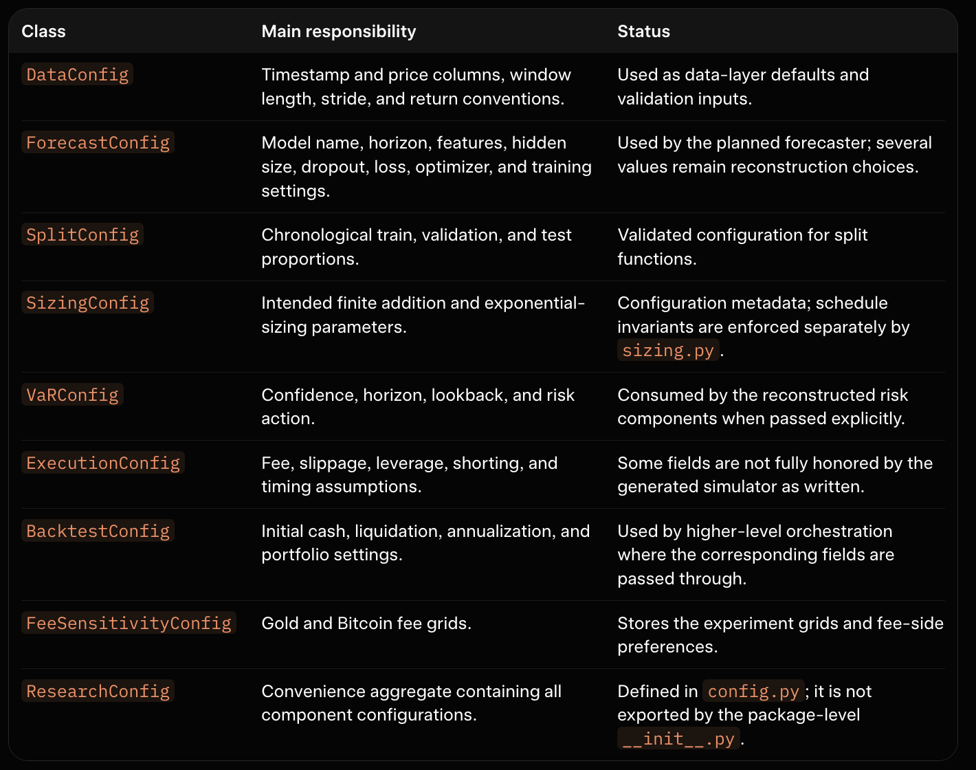
For example, the paper-inspired data and forecasting defaults are:

@dataclass
class DataConfig:
    timestamp_column: str = "timestamp"
    price_column: str = "price"
    window_length: int = 100
    stride: int = 1
    return_definition: str = "simple"


@dataclass
class ForecastConfig:
    model_name: str = "att_bilstm"
    horizon: int = 1
    target_type: str = "scaled_price"
    hidden_size: int = 32
    num_layers: int = 1
    dropout: float = 0.20
    learning_rate: float = 0.001
    optimizer: str = "rmsprop"
    loss: str = "mae"
    learned_attention_query: bool = True

The values with the clearest connection to the paper are:

• window_length=100: the reported historical window length;

• stride=1: the reported one-observation shift between windows;

• dropout=0.20: the paper-inspired dropout rate;

• loss="mae": the reported training loss;

• optimizer="rmsprop": a correction to the paper's terminology, since RMSprop is an optimizer rather than an activation function;

• model_name="att_bilstm": the paper's claimed primary forecasting model.

The hidden size, number of layers, learning rate, batch size, epoch count, early-stopping policy, and learned-query choice are not established by the paper. They are configurable reconstruction choices and should be recorded with any result.

4.2 Make the forecast horizon explicit

The paper's prediction discussion is not consistent about horizon. Its model description and metric table can be read as a one-step forecasting setup, while the conclusion refers to forecasts for the next three days. The source does not establish whether this means a three-element output vector, repeated one-step forecasts, or a single prediction for the third day.

The configuration makes the choice visible:

one_day = ForecastConfig(horizon=1)
three_days = ForecastConfig(horizon=3)

The horizon affects more than the output layer. It changes target construction, prediction metrics, signal aggregation, and execution timing. A one-step model should not be called a three-day model merely because its output is used repeatedly. The selected horizon should be stored in experiment metadata.

target_type is similarly uncertain. The paper does not clearly say whether it predicts raw prices, scaled prices, returns, or percentage changes. The generated default, "scaled_price", is a practical implementation choice and not a verified transcription.

4.3 Position-sizing configuration: metadata versus enforcement

The position-management equations are among the least reproducible parts of the paper. Equations (5) and (6) appear to describe recursive additions intended to compensate for declines and fees, but their notation is corrupted. Equation (7) does not clearly identify the independent variable of the exponential, and Equation (8) appears to normalize position scores into allocations.

SizingConfig records a possible reconstruction:

@dataclass
class SizingConfig:
    maximum_additions: int = 5
    initial_level: int = 1
    growth_rate: float = 0.50
    score_scale: float = 1.0
    allocation_fraction: float = 1.0
    initial_position_fraction: float = 0.20
    maximum_exposure_fraction: float = 1.0
    allow_reuse: bool = False
    calibrate_from_percentiles: bool = False
    recovery_percentile: float = 0.50
    decline_percentile: float = 0.10
    fee_buffer: float = 0.0

The intended normalized reconstruction is:

score_i      = score_scale * exp(growth_rate * i)
weight_i     = score_i / sum(score_j)
allocation_i = budget * weight_i

However, these configuration fields should not be confused with runtime guarantees. In the generated project, sizing.py builds schedules through build_exponential_schedule() and enforces schedule-level properties through SizingSchedule, including finite allocations, normalized weights, a total budget, and one-time level consumption. validate_config() validates maximum_additions and related fractions, but it does not construct a schedule or verify its normalized weights.

Likewise, allocation_fraction, maximum_exposure_fraction, allow_reuse, and fee_buffer are currently configuration or documentation choices rather than completely wired controls in the generated sizing path. The schedule builder receives its own budget and growth arguments. It does not automatically read every corresponding field from SizingConfig, and fee_buffer is not applied to an allocation. A caller must pass the intended values into the sizing module explicitly or add the missing integration before treating them as active controls.

The safe interpretation is therefore:

• maximum_additions documents the intended finite schedule size;

• schedule normalization and budget checks belong to SizingSchedule and sizing.py;

• reuse prevention is enforced when a constructed schedule marks a level as used;

• exposure and cash caps must be applied by the sizer, strategy, or simulator that receives them;

• the incomplete paper equations remain a reconstruction, not an exact implementation.

4.4 VaR configuration is an operational reconstruction

The paper names VaR but does not define its confidence level, horizon, estimation window, return distribution, or action threshold. A usable risk filter must choose all of these values, so VaRConfig makes them explicit:

@dataclass
class VaRConfig:
    enabled: bool = True
    confidence: float = 0.95
    horizon: int = 1
    lookback: int = 100
    method: str = "historical"
    action: str = "scale"
    max_var_fraction: float = 0.05
    insufficient_history: str = "allow"
    min_observations: int = 30

These defaults describe a rolling historical-VaR interpretation, not the paper's verified settings:

• confidence=0.95 selects a 95% lower-tail confidence convention;

• horizon=1 uses one period by default;

• lookback=100 limits the estimation history;

• method="historical" avoids assuming normally distributed returns;

• action="scale" permits reducing an order when projected risk is too high;

• max_var_fraction=0.05 expresses the risk limit as a fraction of portfolio value;

• insufficient_history="allow" defines behavior before enough observations exist.

The generated risk.py contains the actual historical estimator and filter. It must receive returns that were available before the decision timestamp. Configuration alone cannot enforce timestamp ordering. Also, because the paper provides no numerical VaR settings, every backtest should report these values as reconstruction metadata.

A stricter configuration can block trades until sufficient history exists:

risk = VaRConfig(
    confidence=0.99,
    lookback=252,
    min_observations=100,
    action="block",
    insufficient_history="block",
)

4.5 Execution and liquidation: record the intended contract carefully

The paper does not specify whether a signal uses the same closing price, the next opening price, or another execution price. It also does not say clearly whether a fee applies to purchases, sales, or both. The intended execution configuration is:

@dataclass
class ExecutionConfig:
    fee_rate: float = 0.002
    fee_on_buy: bool = True
    fee_on_sell: bool = True
    slippage_rate: float = 0.0
    allow_fractional_units: bool = True
    allow_short: bool = False
    max_leverage: float = 1.0
    execute_next_bar: bool = True
    reject_insufficient_cash: bool = True

These fields describe the desired research contract, but the generated backtest.py does not fully honor all of them as written. In particular:

• the simulator applies fee_rate to both buys and sells unconditionally; it does not consult fee_on_buy or fee_on_sell;

• unaffordable buys are clipped to the affordable quantity rather than being controlled by reject_insufficient_cash;

• the simulator uses its own allow_leverage behavior and does not enforce max_leverage from ExecutionConfig;

• the default simulator is nevertheless long-only and non-leveraged through its separate defaults, so cash and holdings are intended to remain nonnegative;

• next-bar execution is enforced by requiring the fill timestamp to be strictly later than the signal timestamp.

This distinction is important. A configuration field is not proof that the current runtime path consumes it. Until the wiring is corrected, results should state the simulator's actual behavior: two-sided fees, optional slippage, clipping of unaffordable buys, no shorting by default, and strict later-bar execution.

BacktestConfig contains additional lifecycle choices:

@dataclass
class BacktestConfig:
    initial_cash: float = 500.0
    initial_quantity: float = 0.0
    liquidate_at_end: bool = True
    risk_free_rate: float = 0.0
    periods_per_year: int = 252
    currency: str = "USD"

The $500 default resembles the paper's stated per-asset starting allocation, but it does not reproduce the paper's final values. Dates, trades, fees, holdings, and liquidation accounting remain unspecified. liquidate_at_end=True is an explicit implementation choice: it may sell remaining holdings and charge the simulator's sell-side fee. A mark-to-market result without liquidation would be different.

4.6 Fee grids use decimal conventions

The paper lists percentages, while the configuration stores decimal rates:

The conversion is:

0.2% = 0.2 / 100 = 0.002
1.5% = 1.5 / 100 = 0.015

The corresponding defaults are:

@dataclass
class FeeSensitivityConfig:
    gold_rates: tuple[float, ...] = (
        0.002, 0.004, 0.006, 0.008, 0.010, 0.012
    )
    bitcoin_rates: tuple[float, ...] = (
        0.015, 0.020, 0.025, 0.030, 0.035
    )
    apply_to_buys: bool = True
    apply_to_sells: bool = True
    hold_signals_fixed: bool = True

Using 0.2 for a 0.2% fee would represent a 20% rate. The validator checks that rates are finite and lie in the interval [0, 1], but it cannot determine whether a user has confused percentage points with decimal rates. In other words, 0.2 is accepted as a numerically valid rate even though it is probably a unit mistake for this experiment. The decimal convention must therefore be documented and reviewed by the caller.

The fee-side flags are also not fully honored by the generated simulator, which currently charges both sides. hold_signals_fixed describes the sensitivity protocol rather than changing the backtest automatically. If fees affect feasibility or greedy ranking, actions may need to be regenerated for each fee scenario.

4.7 What validate_config() checks

The public validator accepts a complete aggregate or individual components:

from quantitative_trading_model.config import (
    ResearchConfig,
    ForecastConfig,
    validate_config,
)

config = ResearchConfig(
    forecast=ForecastConfig(
        model_name="att_bilstm",
        horizon=3,
        dropout=0.20,
        loss="mae",
        optimizer="rmsprop",
    )
)

validate_config(config)

Component validators check basic constraints such as:

_require(config.window_length > 0, "data.window_length must be positive")
_require(0 <= config.dropout < 1, "forecast.dropout must be in [0, 1)")
_require(0 < config.confidence < 1, "var.confidence must be in (0, 1)")
_require(config.fee_rate >= 0, "execution.fee_rate cannot be negative")
_require(config.maximum_additions > 0, "sizing.maximum_additions must be positive")

This validation rejects invalid configuration values such as nonpositive horizons, dropout outside [0, 1), unsupported optimizer or loss names, split fractions that do not sum to one, negative fees or slippage, invalid VaR actions, and empty fee grids.

It does not perform every runtime or semantic check. Specifically:

• it does not construct a sizing schedule or check that its weights sum to one;

• it does not validate the contents of a price file;

• it does not prove that every configuration field is consumed by the backtest;

• it does not detect a percentage-unit mistake such as entering 0.2 for 0.2%;

• it does not establish that VaR inputs are timestamp-safe;

• it does not verify that generated experiments reproduce the paper.

Schedule-level invariants are handled in sizing.py, data invariants in data.py, and accounting invariants in backtest.py. Those layers must be reviewed together with configuration validation.

The validator also rejects supplying both a complete ResearchConfig and individual component overrides. This prevents a caller from validating one configuration while accidentally running another.

4.8 Record a complete experiment configuration

A complete experiment can combine paper-inspired and reconstructed settings:

from quantitative_trading_model.config import (
    ResearchConfig,
    ForecastConfig,
    VaRConfig,
    validate_config,
)

config = ResearchConfig(
    forecast=ForecastConfig(
        model_name="att_bilstm",
        horizon=3,
        hidden_size=32,
        dropout=0.20,
        loss="mae",
        optimizer="rmsprop",
    ),
    var=VaRConfig(
        confidence=0.95,
        horizon=1,
        lookback=100,
        action="scale",
    ),
)

validate_config(config)

metadata = {
    "window_length": config.data.window_length,
    "stride": config.data.stride,
    "forecast_horizon": config.forecast.horizon,
    "dropout": config.forecast.dropout,
    "loss": config.forecast.loss,
    "optimizer": config.forecast.optimizer,
    "var_confidence": config.var.confidence,
    "var_lookback": config.var.lookback,
    "fee_rate": config.execution.fee_rate,
    "liquidate_at_end": config.backtest.liquidate_at_end,
}

This record combines direct paper-inspired values with reconstruction choices. It should be saved alongside forecast metrics, portfolio metrics, data provenance, and software-version information.

ResearchConfig is available from quantitative_trading_model.config. It is not currently included in the package-level exports in quantitative_trading_model/__init__.py, so importing it from the configuration module is the reliable documented path.

4.9 Configuration is necessary but not sufficient

The configuration contract solves an engineering problem: it makes assumptions visible, validates basic values, and gives experiments a stable record. It does not solve the paper's missing-information problem. It cannot recover:

• the unidentified gold and Bitcoin datasets;

• the original dates, frequency, or test boundary;

• the exact attention query and network architecture;

• the corrupted recursive position-sizing equations;

• the paper's VaR settings or action policy;

• the modified greedy algorithm's objective;

• the original execution, fee, and liquidation protocol;

• the numeric values behind the fee-sensitivity figures.

The approximately $646 gold result, approximately $215,487 Bitcoin result, combined approximately $216,133 result, and reported benchmark metrics therefore remain unverified paper claims. Matching visible defaults does not reproduce those results.

The generated project also has known API inconsistencies between some configuration fields and downstream modules, and semantic code verification was skipped. This section consequently describes the intended configuration contract and the actual validation boundaries; it does not claim that the generated code was executed or that every setting passed through the complete runtime pipeline.

The safest interpretation is that configuration turns an incomplete paper into an auditable research specification. It identifies what comes from the source, what is reconstructed, what is merely illustrative, and which safety controls belong to this educational implementation rather than to the original paper.

5. Load Local Prices Without Assuming the Paper’s Missing Dataset

The paper says that it uses historical gold and Bitcoin prices, but it does not identify the data source, instrument, currency, frequency, date range, or exact columns. That omission is important: even a correct implementation can produce different results if it uses a different gold contract, Bitcoin exchange, timezone, sampling interval, or adjusted-price convention.

The generated project therefore does not silently select a market-data provider. Instead, it accepts a local CSV file or a caller-supplied pandas object. This keeps the experiment offline and makes data provenance the reader’s responsibility. Before treating a result as empirical evidence, record where the file came from, which instrument it represents, and how it was prepared.

5.1 The minimum data contract

The implementation reduces each asset to two essential fields:

• timestamp: when the price observation was available;

• price: a finite, strictly positive price.

A minimal CSV looks like this:

timestamp,price
2020-01-01,1518.2
2020-01-02,1523.7
2020-01-03,1511.4

The PriceData class in src/quantitative_trading_model/data.py stores the cleaned result and an asset label:

@dataclass(frozen=True)
class PriceData:
    frame: pd.DataFrame
    asset: str = "asset"

    def __post_init__(self) -> None:
        required = {"timestamp", "price"}
        missing = required.difference(self.frame.columns)
        if missing:
            raise ValueError(f"PriceData is missing required columns: {sorted(missing)}")

        timestamps = pd.to_datetime(self.frame["timestamp"], errors="raise")
        prices = pd.to_numeric(self.frame["price"], errors="raise").to_numpy(dtype=float)

        if timestamps.duplicated().any():
            raise ValueError("PriceData timestamps must be unique")
        if not timestamps.is_monotonic_increasing:
            raise ValueError("PriceData timestamps must be strictly increasing")
        if not np.isfinite(prices).all() or (prices <= 0).any():
            raise ValueError("PriceData prices must be finite and strictly positive")

PriceData.__post_init__ is a validation boundary. It does not decide whether a price is economically meaningful for every possible instrument, but it enforces the assumptions required by the downstream time-series code. An empty dataset, duplicate timestamp, unsorted timestamp sequence, missing value, infinity, zero, or negative price cannot silently proceed into window construction.

The timestamps and prices properties provide convenient, typed access to the two series:

@property
def timestamps(self) -> pd.DatetimeIndex:
    return pd.DatetimeIndex(self.frame["timestamp"])

@property
def prices(self) -> np.ndarray:
    return self.frame["price"].to_numpy(dtype=float, copy=True)

Returning a copy from prices reduces the chance that a caller accidentally mutates the validated internal frame without re-running validation.

5.2 Standardizing different local column names

Real CSV files often use names such as Date, datetime, Close, or Adj Close. The standardize_prices function accepts explicit column names when necessary, but can also recognize common alternatives:

def standardize_prices(
    data: Union[pd.DataFrame, PriceData],
    *,
    timestamp_column: Optional[str] = None,
    price_column: Optional[str] = None,
    asset: str = "asset",
    drop_invalid: bool = True,
) -> PriceData:

The function first copies the input, so cleaning does not mutate the caller’s DataFrame. It then resolves columns through _resolve_column:

timestamp_column = _resolve_column(
    frame, timestamp_column,
    ("timestamp", "datetime", "date", "time"),
    "timestamp",
)
price_column = _resolve_column(
    frame, price_column,
    ("price", "close", "adj_close", "adjusted_close"),
    "price",
)

Explicit names are safer when a file contains several possible price fields. For example, choosing close versus adjusted_close can materially change a historical experiment. Automatic inference is a convenience, not a substitute for documenting the choice.

The selected columns are renamed to the package’s stable internal names:

normalized = frame[[timestamp_column, price_column]].rename(
    columns={timestamp_column: "timestamp", price_column: "price"}
)
normalized["timestamp"] = pd.to_datetime(
    normalized["timestamp"], errors="coerce", utc=False
)
normalized["price"] = pd.to_numeric(normalized["price"], errors="coerce")

Values that cannot be parsed become missing. The function then constructs a validity mask requiring a real timestamp and a finite, positive price:

valid = normalized["timestamp"].notna() & normalized["price"].notna()
valid &= np.isfinite(normalized["price"].to_numpy(dtype=float))
valid &= normalized["price"] > 0

By default, invalid rows are removed. If drop_invalid=False, the function raises an error instead. The choice depends on the research context: dropping a corrupted row may be reasonable for a demonstration, but a production-quality study should usually stop and investigate why the row is invalid rather than silently deleting it.

5.3 Sorting and duplicate timestamps

After parsing, the function sorts by timestamp using a stable sort and removes duplicate timestamps by retaining the last source row:

normalized = (
    normalized.sort_values("timestamp", kind="mergesort")
    .drop_duplicates("timestamp", keep="last")
    .reset_index(drop=True)
)

This gives the downstream model one price per timestamp. It does not prove that the retained row is the correct observation. If duplicate rows represent separate trades, multiple venues, or different assets, they should be aggregated or separated before calling standardize_prices.

The duplicate policy is therefore an implementation convenience, not a fact recovered from the paper. The paper does not explain how duplicate timestamps or multiple records within one sampling interval were handled.

5.4 Loading a local CSV

load_price_csv is a thin file-system wrapper around standardize_prices:

def load_price_csv(
    path: Union[str, Path],
    *,
    timestamp_column: Optional[str] = None,
    price_column: Optional[str] = None,
    asset: str = "asset",
    drop_invalid: bool = True,
) -> PriceData:
    source = Path(path)
    if not source.exists() or not source.is_file():
        raise FileNotFoundError(f"Price CSV does not exist: {source}")
    if source.suffix.lower() != ".csv":
        raise ValueError("load_price_csv accepts a local .csv file")
    return standardize_prices(
        pd.read_csv(source),
        timestamp_column=timestamp_column,
        price_column=price_column,
        asset=asset,
        drop_invalid=drop_invalid,
    )

The function deliberately accepts only a local .csv path. There are no HTTP requests, exchange clients, credentials, or hidden downloads. This is consistent with the project’s educational and offline scope.

The CLI exposes the same idea through the validate-data subcommand. Its local-path helper rejects URL-like strings before loading them:

def _safe_input_path(value: str) -> Path:
    if "://" in value:
        raise CLIError(
            "Only local files are supported; URLs and network paths are not accepted"
        )
    path = Path(value).expanduser()
    if not path.exists():
        raise CLIError(f"Input file does not exist: {path}")
    if not path.is_file():
        raise CLIError(f"Input path is not a regular file: {path}")
    return path.resolve()

A local validation command can therefore be written as:

quant-trading-model validate-data prices.csv \
  --timestamp-column timestamp \
  --price-column close \
  --asset gold

The command prints or writes a compact summary rather than training a model. This makes data inspection a separate step from forecasting and backtesting.

5.5 Keeping gold and Bitcoin separate

The PriceData representation is intentionally single-asset. A file may contain multiple assets, but the research pipeline should filter it into one chronologically ordered series per asset before creating windows. Gold and Bitcoin have different price scales, trading calendars, liquidity characteristics, and likely data sources. Combining them accidentally into one price sequence would make the next observation after a gold row appear to be a Bitcoin movement.

A multi-asset table can be filtered explicitly:

raw = pd.read_csv("historical_prices.csv")

gold = standardize_prices(
    raw.loc[raw["asset"].eq("gold")],
    timestamp_column="timestamp",
    price_column="price",
    asset="gold",
)

bitcoin = standardize_prices(
    raw.loc[raw["asset"].eq("bitcoin")],
    timestamp_column="timestamp",
    price_column="price",
    asset="bitcoin",
)

Each result can then be passed independently to the window builder and forecasting experiment. This also makes it possible to record asset-specific provenance and fee assumptions. The paper’s headline results allocate $500 to each asset, but the extracted text does not identify whether the assets were sampled on matching dates or evaluated with identical calendars.

5.6 Synthetic data are for interfaces, not validation

Because the paper’s original datasets are unavailable, the project includes generate_synthetic_prices. It creates deterministic, positive price paths using a seeded random generator:

def generate_synthetic_prices(
    *,
    asset: str = "synthetic",
    periods: int = 500,
    start: Union[str, pd.Timestamp] = "2020-01-01",
    seed: int = 7,
    initial_price: Optional[float] = None,
) -> PriceData:

The function chooses different illustrative drift and volatility defaults for labels containing gold or bitcoin, then constructs a positive path from exponentiated random shocks. The seed makes the example repeatable for teaching and invariant checks.

For example:

from quantitative_trading_model.data import generate_synthetic_prices

prices = generate_synthetic_prices(
    asset="gold",
    periods=500,
    seed=7,
)
print(prices.asset)
print(prices.frame.head())

The label-specific behavior is only a teaching convenience. A “Bitcoin-like” synthetic path is not Bitcoin data, and a “gold-like” path is not a gold instrument. Synthetic data can demonstrate that timestamps, windows, attention tensors, sizing budgets, and portfolio accounting have compatible interfaces. It cannot validate the paper’s forecast metrics, fee curves, or reported final values.

5.7 Data checks before modeling

Before moving to sliding windows, record at least the following:

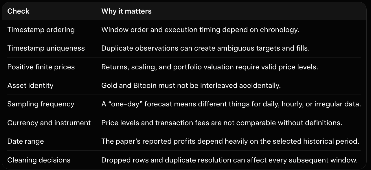
The generated tests in tests/test_data_and_streaks.py are intended to check these kinds of invariants with small hand-built fixtures. They are static artifacts in this project review; no claim is made here that the generated test suite was executed successfully.

The essential principle is simple: clean only what the data contract justifies, preserve timestamps, separate assets, and document every assumption before training. Once the local series is trustworthy and its provenance is recorded, the next step is to construct the paper’s 100-observation windows without allowing scaling or temporal partitioning to leak future information.

6. Build Leakage-Safe Sliding Windows

The paper describes a sliding-window forecasting setup with a history of 100 observations and a stride of one. The model reads the latest 100 observations, predicts a later value, advances one observation, and creates the next overlapping example.

The important issue is not only the window size. Every forecast must use information available at its decision timestamp. The target must occur after the input window, scaling parameters must be fitted without future observations, and evaluation must preserve chronological order.

6.1 The one-step relationship

Let z_t denote a transformed price or feature value at time t. With a window length of 100, a one-step sample is:

\[ Xt = [z{t-99}, z{t-98}, \ldots, z{t-1}, zt], \qquad yt = z_{t+1}. \]

The final value in X_t is the latest information available when the forecast is generated. The target belongs to the next observation.

The paper-inspired window settings are represented by DataConfig:

@dataclass
class DataConfig:
    timestamp_column: str = "timestamp"
    price_column: str = "price"
    window_length: int = 100
    stride: int = 1

window_length=100 and stride=1 come from the paper. The paper does not clearly state whether the model uses raw prices, normalized prices, returns, or additional features, so the representation remains an explicit implementation choice.

6.2 How make_windows constructs samples

The central function is make_windows in src/quantitative_trading_model/data.py. It accepts a cleaned PriceData object, a DataFrame, or a numeric array. For timestamp-aware inputs, it stores the start, end, and target timestamps alongside the arrays.

The core operation is equivalent to:

for start in range(0, last_start + 1, stride):
    end = start + window_length - 1
    X.append(transformed[start : end + 1])
    targets.append(transformed[end + 1 : end + 1 + horizon, 0])
    target_times.append(timestamps[end + horizon])

With the defaults, the first sample contains observations 0 through 99 and targets observation 100. The next sample contains observations 1 through 100 and targets observation 101.

The returned WindowedDataset includes temporal metadata:

@dataclass(frozen=True)
class WindowedDataset:
    X: np.ndarray
    y: np.ndarray
    window_start: pd.DatetimeIndex
    window_end: pd.DatetimeIndex
    y_timestamp: pd.DatetimeIndex
    feature_names: Tuple[str, ...] = ("price",)

Its invariant check requires every target timestamp to follow the corresponding input window:

if n and not (self.y_timestamp > self.window_end).all():
    raise ValueError("Every target timestamp must be after its input window")

This timestamp guarantee applies when the input carries timestamps, such as PriceData or a cleaned DataFrame. For a raw numeric array, the current implementation has no timestamp argument in that code path and creates placeholder daily timestamps beginning at 1970-01-01. Those generated timestamps preserve array alignment for shape-based demonstrations, but they are not source-market timestamps. A trading experiment should therefore use PriceData or a timestamp-aware DataFrame.

6.3 One-day versus three-day targets

The paper is ambiguous about the forecast horizon. Its prediction discussion is compatible with one-step forecasting, while its conclusion refers to forecasts for the next three days. The implementation exposes horizon rather than silently choosing one interpretation.

For horizon=1:

X.shape = (samples, 100, features)
y.shape = (samples,)

For horizon=3:

\[ yt = [z{t+1}, z{t+2}, z{t+3}]. \]

The shape is then:

X.shape = (samples, 100, features)
y.shape = (samples, 3)

The final target timestamp is the timestamp of z_{t+3}. Converting a three-value forecast into a buy, sell, or hold decision belongs to the strategy layer. Possible rules include using the terminal forecast, the mean forecast, or a separately specified multi-day signal.

For a series of N observations, the number of stride-one windows is:

N−100−h+1,

where h is the forecast horizon. The final window must leave enough observations for every target value.

6.4 Overlapping windows and temporal partitions

Stride one creates heavily overlapping samples:

window 1: [0, 1, 2, ..., 99] -> target 100
window 2: [1, 2, 3, ..., 100] -> target 101

This overlap is normal for sliding-window forecasting. The risk comes from treating neighboring samples as independent random observations. If windows are randomly shuffled before splitting, almost identical histories can appear in both partitions, producing optimistic estimates.

The generated recurrent training code therefore uses non-shuffled batches:

train_loader = DataLoader(
    TensorDataset(torch.from_numpy(x_train), torch.from_numpy(y_train)),
    batch_size=batch_size,
    shuffle=False,
)

chronological_split also preserves sample order. This prevents random cross-partition mixing, but it does not guarantee that raw input histories are disjoint at the boundary. The final training window and first test window may still share observations because the windows overlap by design. That dependence should be acknowledged when interpreting metrics; walk-forward evaluation and a documented gap can provide a stricter protocol.

6.5 Fit scaling on training observations only

Scaling can make neural-network optimization easier, but fitting a scaler on the complete series leaks future distribution information. For example, a full-series min-max scaler exposes the training process to the future minimum and maximum.

The repository provides ChronologicalScaler:

scaler = ChronologicalScaler()
scaler.fit(training_values)                 # training rows only
train_scaled = scaler.transform(train_values)
test_scaled = scaler.transform(test_values)

The safe sequence is:

Clean and sort the complete local file.

Establish the chronological raw-row training boundary.

Fit the scaler only on rows before that boundary.

Transform later rows with the fitted scaler.

Build windows and retain their timestamps.

Inverse-transform predictions before reporting price-level metrics when appropriate.

make_windows accepts an already fitted scaler. Its fit_scaler option is intended for controlled demonstrations; setting fit_scaler=True on the complete dataset before an out-of-sample experiment would leak future information. The window builder does not know whether the caller selected a valid training boundary and cannot enforce this policy automatically.

A safer pattern is:

train_rows = price_data.frame.iloc[:training_row_count]
scaler = ChronologicalScaler().fit(
    train_rows[["price"]].to_numpy(dtype=float)
)

windows = make_windows(
    price_data,
    window_length=100,
    horizon=1,
    stride=1,
    scaler=scaler,
    fit_scaler=False,
)

Here, training_row_count must be determined from a documented chronological rule, such as a date boundary or a fixed initial training period. It must not be chosen after inspecting test performance. If windows are built from the entire transformed series and then split, the scaler remains training-fitted, but boundary overlap still exists; a stricter workflow can build or select partitions around an explicit raw-row boundary.

6.6 Chronological 70:30 splitting

The paper reports a 70:30 train/test split. The implementation provides chronological_split for a paper-style comparison:

train, test = chronological_split(
    dataset,
    train_fraction=0.70,
    validation_fraction=0.0,
)

The function slices ordered samples rather than randomly selecting indices. With validation data, the order is:

training windows -> validation windows -> test windows

The metadata-preserving helper is conceptually:

def dataset_slice(dataset, start, stop):
    return WindowedDataset(
        X=dataset.X[start:stop],
        y=dataset.y[start:stop],
        window_start=dataset.window_start[start:stop],
        window_end=dataset.window_end[start:stop],
        y_timestamp=dataset.y_timestamp[start:stop],
        feature_names=dataset.feature_names,
    )

A useful ordering check is:

train_times = train.y_timestamp
test_times = test.y_timestamp
assert train_times.max() < test_times.min()

This confirms that target timestamps are ordered across the sample split. It does not prove that the corresponding input histories are disjoint, because stride-one windows can overlap at the boundary.

The exact boundary remains a reconstruction. The paper does not specify the split date or whether it splits raw observations before window construction or partitions already-created windows. Those choices can produce different edge behavior and should be recorded in experiment metadata.

6.7 Walk-forward evaluation for trading conclusions

A single 70:30 split answers only how one fixed training period performs on one later period. It does not show how results change as new observations arrive.

An expanding walk-forward procedure repeatedly preserves the information boundary:

train on [0, ..., t]
forecast the next block
advance the boundary
expand the training set
forecast the next block
repeat

The walk_forward_splits generator is used like this:

for train, validation, test in walk_forward_splits(
    dataset,
    initial_train_size=500,
    validation_size=0,
    test_size=20,
    step=20,
):
    # Fit only on train, optionally tune on validation,
    # then evaluate on the later test block.
    pass

Each test block follows its training block. The training set expands over time; a rolling fixed-length training window would be another explicit choice.

The paper does not report walk-forward results, so such results are not reproductions of its tables. They are a more appropriate protocol for trading conclusions because they repeatedly test the model on observations that follow the fitting period.

6.8 What the generated test artifact actually demonstrates

The generated tests/test_data_and_streaks.py uses a compatibility helper with a numeric price array and a separate timestamp object. In the current make_windows implementation, the numeric-array path does not accept or preserve that separate timestamp argument; it creates placeholder daily timestamps. Therefore, the test's meaningful checks are the numeric window boundaries and target values, while its timestamp behavior should not be interpreted as validation of real source timestamps.

A timestamp-aware illustrative example, using the public data contract directly, is:

prices = np.arange(10.0, 17.0)
timestamps = pd.date_range(
    "2024-01-01", periods=len(prices), freq="D"
)
price_data = PriceData(
    pd.DataFrame({"timestamp": timestamps, "price": prices})
)

dataset = make_windows(
    price_data,
    window_length=3,
    horizon=1,
    stride=1,
)

np.testing.assert_allclose(dataset.y, prices[3:])
assert (dataset.y_timestamp > dataset.window_end).all()

This is an illustrative contract for timestamp-aware input, not a claim that the generated test suite was executed. It also makes the distinction clear: use PriceData or a timestamp-aware DataFrame when timestamps matter; use raw arrays only when placeholder metadata is acceptable or when a higher-level API supplies the timestamp mapping separately.

The project was reviewed primarily through static checks, and semantic code verification was skipped. The intended contracts are described here, but this section does not claim that the complete test suite passed or that runtime behavior was independently confirmed.

6.9 Practical preparation workflow

For a local asset file, a disciplined workflow is:

price_data = load_price_csv(
    "data/gold.csv",
    timestamp_column="timestamp",
    price_column="price",
    asset="gold",
)

# Establish this from a documented date or raw-row boundary.
training_row_count = 500
train_rows = price_data.frame.iloc[:training_row_count]
scaler = ChronologicalScaler().fit(
    train_rows[["price"]].to_numpy(dtype=float)
)

windows = make_windows(
    price_data,
    window_length=100,
    horizon=1,       # use 3 only when a three-step target is intended
    stride=1,
    scaler=scaler,
    fit_scaler=False,
)
train, test = chronological_split(windows, train_fraction=0.70)

The row boundary must be established before fitting the scaler and must reflect the intended training period. The split shown above is a paper-style sample split applied after window construction. For a stricter out-of-time study, define the raw-row boundary and any gap explicitly, then use walk-forward partitions for repeated evaluation.

6.10 Preparation limits

This data layer provides:

• the paper's 100-observation, stride-one setup;

• one-step and three-step target shapes;

• timestamp metadata for PriceData and timestamp-aware DataFrame inputs;

• chronological ordering and sample splits;

• training-only scaling primitives;

• expanding walk-forward partitions.

It does not resolve the paper's missing data source, instrument definition, feature representation, exact split date, forecast horizon, or execution protocol. It also cannot automatically determine whether a caller fitted a scaler on an appropriate subset or whether overlapping input histories are acceptable for a particular evaluation design.

The essential causal contract is therefore: the historical window ends first, the target occurs later, scaling uses only the declared training information, and execution is aligned to a timestamp after the information endpoint. Later forecasting and backtesting layers should preserve that contract explicitly.

7. Keep Forecast Accuracy Separate from Trading Performance

The paper compares forecasting models with RMSE, MAE, MAPE, and R-squared. These metrics answer one question: how close were the predictions to their targets? They do not establish that a trading strategy is profitable after signal rules, position sizing, VaR, execution timing, fees, slippage, and liquidity are included.

The implementation keeps these concerns separate in src/quantitative_trading_model/metrics.py:

• forecast metrics operate on target and prediction arrays;

• portfolio metrics operate on a marked-to-market value path and optional execution records;

• backtest.py supplies the fills, traded notionals, and fees used by portfolio reporting.

This distinction is also documented in README.md, which warns that forecast accuracy does not establish profitability and recommends reporting drawdown, volatility, turnover, fees, and a buy-and-hold comparison.

7.1 Forecast error metrics

Let y_k be the observed target and y_hat_k the corresponding prediction for evaluation item k.

Mean absolute error

\( \operatorname{MAE} = \frac{1}{N}\sum{k=1}^{N}|yk-\hat y_k|. \)

MAE is measured in the target's units. For raw dollar prices, it is measured in dollars. The paper-inspired recurrent models also use MAE as their training loss.

Root mean squared error

\(\operatorname{RMSE} = \sqrt{\frac{1}{N}\sum{k=1}^{N}(yk-\hat y_k)^2}. \)

Squaring the residuals gives larger errors more influence. RMSE is scale-dependent, so raw RMSE values for gold and Bitcoin should not be compared without considering their different price magnitudes and target representations.

Mean absolute percentage error

\( \operatorname{MAPE} = \frac{100}{N}\sum{k=1}^{N}\left|\frac{yk-\hat yk}{yk}\right|. \)

The implementation reports MAPE in percentage points: 2.5 means 2.5%, not 0.025. MAPE is undefined or unstable for zero and near-zero targets. forecast_metrics therefore exposes two controls:

• mape_epsilon defines the near-zero threshold;

• mape_zero_policy="exclude" omits those targets, while "raise" rejects them.

The number of observations included in MAPE is stored separately from the total sample count. Two MAPE values should not be compared without checking that policy and count.

R-squared

\(R^2 = 1 - \frac{\sumk(yk-\hat yk)^2}{\sumk(y_k-\bar y)^2}. \)

R-squared compares residual variation with the variation of the targets around their mean. It can be negative when predictions are worse than the constant mean-target baseline. If every target is identical, the denominator is zero; the generated implementation returns 1.0 for an exact prediction and 0.0 otherwise.

7.2 The forecast-metrics interface

The public function is forecast_metrics(actual, predicted, ...). It validates finite inputs, flattens supported array-like values, checks that targets and predictions have equal lengths, and returns a ForecastMetrics dataclass.

The following is a shortened tutorial excerpt, not the complete generated source. The actual module also contains helper functions for input validation, rounding, and serialization.

metrics = forecast_metrics(
    actual,
    predicted,
    mape_epsilon=1e-12,
    mape_zero_policy="exclude",
)

print(metrics.rmse)
print(metrics.mae)
print(metrics.mape_percent)
print(metrics.r_squared)
print(metrics.as_dict())

ForecastMetrics.as_dict() is the generated dataclass's serialization method. It includes the four metrics, sample counts, the MAPE threshold, and the selected MAPE policy. The full implementation should be treated as authoritative rather than this abbreviated excerpt.

For example:

import numpy as np
from quantitative_trading_model.metrics import forecast_metrics

actual = np.array([100.0, 110.0, 90.0])
predicted = np.array([102.0, 107.0, 93.0])

result = forecast_metrics(actual, predicted)

The residuals are [2, -3, 3]. Thus MAE is 8/3, RMSE is sqrt(22/3), and MAPE is the mean of the three absolute relative errors multiplied by 100. These values describe only the prediction sample. They do not determine whether a strategy would buy, sell, or hold.

For multi-step predictions represented as (samples, horizon), the generated metric helper flattens the arrays. The caller must ensure that the target and prediction arrays have identical ordering. A production experiment should also retain target timestamps so that metrics are calculated on aligned observations.

7.3 Why forecast accuracy is not trading performance

A model can have favorable forecast errors and still produce a poor trading result:

A predicted move may be too small to cover entry and exit costs.

Price-level accuracy does not guarantee correct direction relative to the current price.

A forecast evaluated at a closing timestamp may not describe the price available at execution.

Position sizing can amplify a small forecast error.

A shuffled or otherwise optimistic time-series split may not represent deployment conditions.

Fees, spreads, slippage, partial fills, and liquidity are portfolio effects, not components of RMSE or MAE.

The paper reports strong Att-BiLSTM forecasting metrics, but those reported values remain unverified claims because the source data, preprocessing, target definition, and test protocol are unavailable. Even reproducing the metric ranking would not prove that the resulting trading strategy is profitable.

7.4 Portfolio metrics use a different vocabulary

Portfolio evaluation begins with marked-to-market values:

\( Vt = \operatorname{cash}t + \operatorname{quantity}t pt. \)

The generated implementation reports or supports the following measures.

Cumulative return

\[ R{0:T} = \frac{VT}{V_0}-1. \]

This reflects trades, fees, remaining holdings, and the configured liquidation policy.

Drawdown and maximum drawdown

\[ Dt = \frac{Vt}{\max{s\le t}Vs}-1. \]

Drawdown is non-positive: -0.25 means the portfolio is 25% below its previous running peak. Maximum drawdown is the minimum value in the drawdown series.

Volatility

For periodic returns r_t, annualized volatility is approximately:

\[ \sigma{annual}=\operatorname{std}(rt)\sqrt{P}, \]

where P is the configured number of periods per year. The default of 252 is an implementation assumption for daily observations, not a paper-specified value.

Sharpe ratio

\[ \operatorname{Sharpe} = \frac{\operatorname{mean}(rt-r{f,t})} {\operatorname{std}(rt-r{f,t})}\sqrt{P}. \]

The implementation converts an annual risk-free rate into a periodic compound-equivalent rate. Its default risk-free rate is zero, another explicit evaluation choice rather than a paper result.

Turnover and fees

The generated metrics layer defines turnover as traded notional divided by mean portfolio value:

\[ \operatorname{turnover} = \frac{\sumi \operatorname{traded\ notional}i}{\operatorname{mean}(V_t)}. \]

Fees are supplied by the execution layer and summed separately:

\[ \operatorname{total\ fees}=\sumi\operatorname{fee}i. \]

This preserves the distinction between portfolio valuation and fill-level accounting.

7.5 The portfolio-metrics interface

portfolio_metrics accepts a value path and optional periodic returns, traded notionals, fees, annualization frequency, and annual risk-free rate. The following is a shortened excerpt, not a complete copy of metrics.py:

portfolio = portfolio_metrics(
    portfolio_values,
    returns=None,              # derive returns from consecutive values
    traded_notionals=notionals,
    fees=fees,
    periods_per_year=252,
    risk_free_rate_annual=0.0,
)

print(portfolio.cumulative_return)
print(portfolio.maximum_drawdown)
print(portfolio.annualized_volatility)
print(portfolio.sharpe_ratio)
print(portfolio.turnover)
print(portfolio.total_fees)

The full generated function additionally validates positive portfolio values, finite inputs, return-length conventions, nonnegative notionals, scalar-versus-sequence fee inputs, and risk-free-rate settings. It returns a PortfolioMetrics dataclass with an as_dict() method.

7.6 A report should retain both layers

A useful experiment table keeps forecast and portfolio results in separate columns:

| Forecast evaluation | Portfolio evaluation | | --- | --- | | RMSE | Final value | | MAE | Cumulative return | | MAPE and MAPE policy | Maximum drawdown | | R-squared | Annualized volatility | | Target horizon | Sharpe ratio | | Test timestamps | Turnover | | Scaling metadata | Total fees |

This prevents a low prediction error from being mistaken for a trading objective. A buy-and-hold benchmark should also use the same asset, period, initial capital, fee convention, and valuation policy.

7.7 Verification scope

The supplied project currently does not include a dedicated metrics test module. tests/test_data_and_streaks.py tests data preparation and streak behavior; it does not directly test MAPE policies, constant-target R-squared behavior, drawdown calculations, or fee aggregation. Those behaviors are documented and statically inspectable invariants, not claims of executed test coverage.

Static review can still check that:

• forecast arrays are finite and aligned;

• MAPE has an explicit near-zero policy;

• constant-target R-squared behavior is deterministic;

• portfolio values are positive and drawdown is non-positive;

• turnover and fees are supplied separately from forecast errors.

However, semantic code verification was skipped, and the generated project was not claimed to have been executed. These checks therefore do not establish runtime correctness, profitability, or reproduction of the paper's metrics.

The practical rule is: use forecast metrics to evaluate the predictor and portfolio metrics to evaluate the trading system. Both are necessary, but neither is a substitute for the other.

8. Implement the Attention-Enhanced BiLSTM

The paper identifies an attention-enhanced bidirectional LSTM, or Att-BiLSTM, as its primary forecasting model. Its intended flow is:

Read a historical window, such as the latest 100 observations.

Process that window in both temporal directions with a BiLSTM.

Produce one hidden representation for every time step.

Use attention to assign larger weights to more relevant historical steps.

Combine the weighted representations into one context vector.

Map that context vector to a one-day or multi-day forecast.

The generated implementation follows this structure in src/quantitative_trading_model/models/forecasters.py. The attention mathematics is isolated in src/quantitative_trading_model/models/attention.py, while tests/test_model_shapes.py checks the intended tensor contracts when the optional PyTorch dependency is available.

Reconstruction boundary: The paper specifies the broad Att-BiLSTM idea, dot-product attention, 20% dropout, MAE, and RMSprop. It does not specify the number of recurrent layers, hidden dimensions, attention-query construction, learning rate, training duration, or exact target representation. Those details are configurable implementation choices, not verified transcriptions of the original model.

8.1 What the BiLSTM contributes

An ordinary LSTM processes a sequence in one direction. Given an input window ordered from older to newer observations, its hidden state at time step i summarizes the observations up to that point in the forward direction.

A BiLSTM adds a second LSTM that processes the same historical window in reverse. At each time step, the model combines the forward and backward states. If the one-direction hidden size is h, the combined representation commonly has size 2h:

input sequence:       (batch, time, features)
forward LSTM states:  (batch, time, h)
backward LSTM states: (batch, time, h)
combined states:      (batch, time, 2h)

The important timing condition is that the complete window must end at the information timestamp. If the signal is generated after observing time t, the input may contain observations through t, but not t+1 or any later observation. The backward LSTM is not automatically leakage because it looks backward inside the already available window. It becomes leakage only if the window itself contains future observations.

The model therefore relies on the contract established by the data layer:

window ends at t
forecast is generated using data through t
execution occurs at a later bar

This is why the window metadata and timestamp checks discussed in the previous section matter to the neural model as well as to the backtest.

8.2 Dot-product temporal attention

The BiLSTM produces a sequence of hidden representations rather than one final vector. The paper's attention mechanism decides how to combine those representations.

Let x_i be the BiLSTM representation at time step i, and let q be a query vector. The paper gives the following operations.

Compatibility score

\[ S(xi,q) = xi^Tq. \]

This dot product produces one scalar score for every time step. A larger score indicates stronger alignment between x_i and the query q.

Attention weights

The scores are normalized with a softmax:

\[ ai = \operatorname{softmax}i(S(xi,q)) = \frac{\exp(S(xi,q))} {\sumj \exp(S(xj,q))}. \]

The subscript on softmax is important. Normalization must happen over the time dimension, so that the weights for one sequence sum to one across its historical observations. Normalizing across features or across the batch would produce a different mechanism.

Context vector

Finally, the representations are combined with their attention weights:

\[ \operatorname{context}(q,x)=\sumi ai x_i. \]

For a batch of sequences, the expected tensor shapes are:

sequence:  (batch, time, feature_dim)
scores:    (batch, time)
weights:   (batch, time)
context:   (batch, feature_dim)
forecast:  (batch, horizon)

The implementation uses DotProductTemporalAttention for these operations:

# src/quantitative_trading_model/models/attention.py

class DotProductTemporalAttention(nn.Module):
    def forward(
        self,
        sequence: Tensor,
        query: Optional[Tensor] = None,
        *,
        return_weights: bool = False,
    ) -> Tensor | Tuple[Tensor, Tensor]:
        self._validate_sequence(sequence)
        prepared_query = self._prepare_query(sequence, query)

        # Equation (1): one dot product per time step.
        scores = torch.einsum("btd,bd->bt", sequence, prepared_query)

        # Equation (2): normalize across time, not features or batches.
        weights = torch.softmax(scores, dim=1)

        # Equation (3): weighted sum of sequence representations.
        context = torch.sum(weights.unsqueeze(-1) * sequence, dim=1)

        self._last_attention_weights = weights
        if return_weights:
            return context, weights
        return context

The Einstein summation expression "btd,bd->bt" means:

• b: batch item;

• t: time step;

• d: feature dimension;

• the feature dimension is multiplied and summed away;

• the result retains batch and time, producing one score per time step.

The next line, torch.softmax(scores, dim=1), is the key implementation detail. For a tensor shaped (batch, time), dimension 1 is time. The result has one probability-like weight for every historical position.

8.3 The unspecified query vector

The paper uses a query vector q in its equations but does not explain where that vector comes from. This missing detail affects the architecture, so the implementation makes the choice explicit rather than hiding it.

DotProductTemporalAttention supports two modes:

• a learned query, stored as a trainable parameter and used by default;

• a caller-provided query, useful for experiments with another interpretation.

The learned-query choice is visible in the constructor:

# src/quantitative_trading_model/models/attention.py

if learned_query:
    query = torch.empty(self.feature_dim)
    nn.init.normal_(query, mean=0.0, std=float(query_init_scale))
    self.query = nn.Parameter(query)
else:
    self.register_parameter("query", None)

When no explicit query is supplied, _prepare_query retrieves the learned vector and broadcasts it across the batch. When a query is supplied, the method checks its dimensionality, device, data type, and finiteness before using it.

This is a sound interface decision for an educational implementation, but it must be labeled correctly:

The learned query is a reconstruction of an unspecified paper detail. It is not evidence that the original authors used a learned query rather than a final hidden state, a separate projection, or another query-generation mechanism.

8.4 From sequence states to a forecast

The primary model in forecasters.py first creates a bidirectional LSTM whose batch_first=True input convention is (batch, time, features):

# src/quantitative_trading_model/models/forecasters.py

self.encoder = nn.LSTM(
    input_size=input_size,
    hidden_size=hidden_size,
    num_layers=num_layers,
    batch_first=True,
    dropout=recurrent_dropout,
    bidirectional=True,
)

self.dropout = nn.Dropout(dropout)
self.attention = DotProductTemporalAttention(self.output_size)
self.head = nn.Linear(self.output_size, horizon)

self.output_size is hidden_size * 2, because the forward and backward states are concatenated. The dense head converts the attention context into the requested forecast horizon. For example:

horizon = 1  -> output shape (batch, 1)
horizon = 3  -> output shape (batch, 3)

The forward pass is intentionally short because each responsibility is delegated to a clear layer:

class AttBiLSTMForecaster(nn.Module):
    def forward(self, inputs: Tensor) -> Tensor:
        _validate_input_tensor(inputs)
        sequence, _ = self.encoder(inputs)
        sequence = self.dropout(sequence)

        context = self.attention(sequence)
        return self.head(self.dropout(context))

Conceptually, this is:

historical window
    -> bidirectional LSTM sequence states
    -> dropout on sequence states
    -> temporal dot-product attention
    -> context vector
    -> dropout on context
    -> linear forecast head

The exact generated implementation also retains the latest attention weights when the attention layer exposes them. That is useful for inspection and debugging, but attention weights should not automatically be interpreted as a complete causal explanation of the prediction.

8.5 Dropout, MAE, and RMSprop

The paper reports a dropout rate of 20%, represented by the default dropout=0.20. Dropout randomly suppresses a fraction of activations during training, which can reduce reliance on a narrow set of internal features. The paper's wording does not establish whether its 20% applies to ordinary feed-forward dropout, recurrent dropout, or both, so the generated code uses explicit nn.Dropout layers and documents the recurrent-layer behavior.

The training function uses MAE loss:

criterion = nn.L1Loss()

This corresponds to:

\[ \operatorname{MAE} = \frac{1}{N}\sumk |yk-\hat y_k|. \]

The optimizer is RMSprop:

optimizer = torch.optim.RMSprop(
    model.parameters(),
    lr=learning_rate,
)

This corrects an important terminology issue in the paper interpretation. RMSprop is an optimizer, not an activation function. It controls how model parameters are updated after gradients are calculated. The activation behavior of the recurrent cells and the linear output head is a separate architectural matter.

The implementation keeps learning rate, hidden size, number of layers, batch size, epochs, and patience configurable because the paper does not provide enough information to hard-code them as original values.

8.6 Why the model trains on chronological batches

train_forecaster constructs a DataLoader with shuffle=False:

train_loader = DataLoader(
    TensorDataset(
        torch.from_numpy(x_train),
        torch.from_numpy(y_train),
    ),
    batch_size=batch_size,
    shuffle=False,
)

Adjacent sliding windows are highly dependent because they share most of their observations. Turning off shuffling preserves the temporal order and makes the training protocol easier to audit. This does not remove all dependence between windows, but it avoids adding a separate randomization step that could make the time-series experiment harder to interpret.

This is a conservative engineering choice rather than a claim that the paper used the same batching policy. The paper mentions shuffled or randomly arranged training behavior in places, but does not provide enough detail to establish a reproducible protocol. For trading conclusions, chronological and walk-forward evaluation remain more important than reproducing an unclear shuffling choice.

8.7 Model-shape checks

The generated tests focus on architecture contracts rather than empirical performance. For example, tests/test_model_shapes.py checks that a configured attention layer returns the expected context shape and that its weights normalize across time:

@pytest.mark.skipif(not TORCH_AVAILABLE, reason="PyTorch is an optional dependency")
class TestAttentionShapes:
    def test_attention_weights_are_normalized_across_time(self) -> None:
        attention = _construct_attention()
        sequence = torch.randn(3, 7, 8)
        output = attention(sequence)
        _, weights = _unpack_attention_output(output)

        if weights is None:
            weights = getattr(attention, "last_attention_weights", None)

        assert tuple(weights.shape) == (3, 7)
        assert torch.isfinite(weights).all()
        assert torch.all(weights >= 0)
        assert torch.allclose(
            weights.sum(dim=1),
            torch.ones(3),
            atol=1e-5,
        )

The test expresses the mathematical invariant directly:

weights.shape == (batch, time)
weights >= 0
sum(weights over time) == 1

Additional shape tests check one-step and three-step outputs:

@pytest.mark.parametrize("horizon", [1, 3])
def test_attention_bilstm_output_horizon(self, horizon: int) -> None:
    model = _construct_forecaster("AttBiLSTMForecaster", horizon=horizon)
    inputs = torch.randn(2, 100, 3)
    predictions = _model_output(model, inputs)

    assert predictions.shape[0] == 2
    assert predictions.shape[-1] == horizon

These checks do not demonstrate that the model matches the paper's forecast metrics. They only verify the intended tensor interface and attention normalization when the optional dependency is installed. The local verification record should therefore be read as static and structural evidence, not as a claim that the model was executed successfully or that the paper's numerical results were reproduced.

8.8 What is direct and what is reconstructed here?

The implementation status of this model can be summarized as follows:

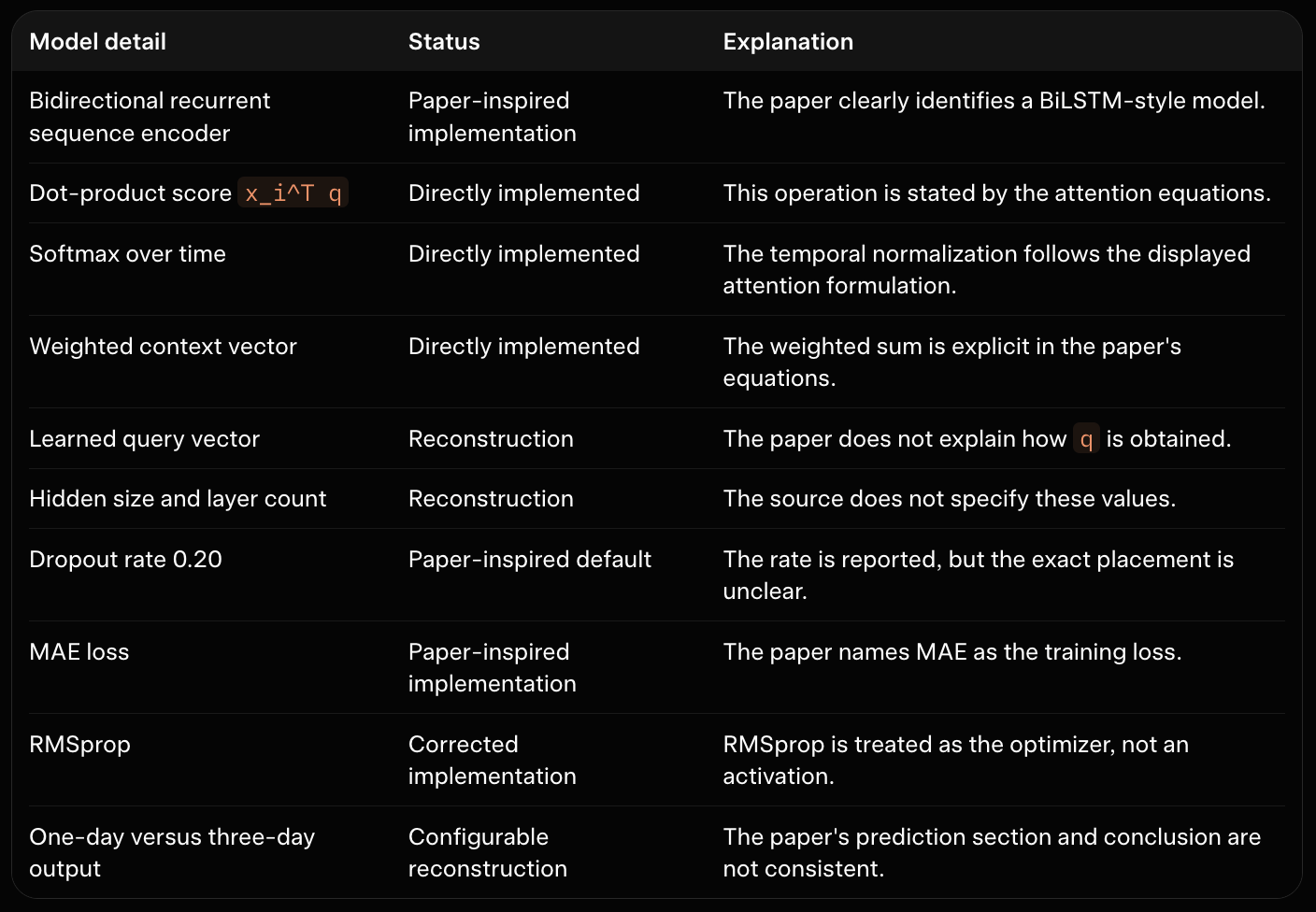
The model is therefore a useful translation of the paper's stated architecture, but not a verified reproduction of its original neural network. Exact comparison would require the original data, preprocessing, target definition, full architecture, training hyperparameters, and untouched evaluation protocol.

9. Walk Through Attention, Training, and Prediction Functions

This section follows the generated Python implementation from tensor validation through attention, recurrent encoding, training, and prediction. The primary model is an attention-enhanced bidirectional LSTM, or Att-BiLSTM. The paper specifies the broad architecture, 20% dropout, MAE loss, and RMSprop optimization, but it does not specify several architectural and training details. Those details remain explicit reconstruction choices.

The examples below describe the generated interfaces and intended invariants. They do not claim that the code was executed, that the tests passed, or that the paper's empirical results were reproduced.

9.1 Optional PyTorch imports

PyTorch is an optional dependency. The data, streak, sizing, risk, and portfolio components are intended to remain usable without installing the deep-learning stack. The model modules therefore import PyTorch conditionally:

try:
    import torch
    from torch import Tensor, nn
except ImportError:
    torch = None
    Tensor = Any
    nn = type("nn", (), {"Module": _ModuleFallback})

The fallback permits the module to be imported in a minimal installation. Constructing DotProductTemporalAttention or a recurrent forecaster still requires PyTorch and raises a clear ImportError if it is unavailable. This is preferable to silently substituting a different model.

The package initializer is also side-effect free. Importing quantitative_trading_model does not load market data, train a model, access a network, or create a trading connection.

9.2 The attention layer's tensor contract

DotProductTemporalAttention expects a sequence tensor with shape:

(batch, time, feature_dim)

For the paper-inspired data setup, time is normally 100. The feature dimension is the size of each recurrent representation. A bidirectional LSTM commonly produces a representation whose width is twice its hidden size because its forward and backward states are concatenated.

The attention layer returns a context tensor with shape:

(batch, feature_dim)

Attention weights have shape:

(batch, time)

They can be returned explicitly or inspected after a forward pass. The weights are useful for diagnostics and shape tests, but they should not automatically be treated as a complete causal explanation of the model.

9.3 Constructing attention and representing the missing query

The paper gives the score equation

\[ S(xi,q)=xi^Tq, \]

but does not explain how the query vector q is created. The constructor exposes this ambiguity:

class DotProductTemporalAttention(nn.Module):
    def __init__(
        self,
        feature_dim: Optional[int] = None,
        *,
        input_dim: Optional[int] = None,
        learned_query: bool = True,
        query_init_scale: float = 0.02,
    ) -> None:
        ...

feature_dim and input_dim are aliases. If both are supplied, they must agree. The dimension must be a positive integer because the unprojected dot product requires the query and sequence representations to have the same width.

With learned_query=True, the layer creates a trainable query parameter:

if learned_query:
    query = torch.empty(self.feature_dim)
    nn.init.normal_(query, mean=0.0, std=float(query_init_scale))
    self.query = nn.Parameter(query)
else:
    self.register_parameter("query", None)

The learned query is a reconstruction choice, not a verified detail from the paper. With learned_query=False, the caller must provide a query to every forward call.

9.4 Validating the sequence tensor

Before computing attention scores, _validate_sequence checks the input shape and values:

def _validate_sequence(self, sequence: Tensor) -> Tuple[int, int, int]:
    if sequence.ndim != 3:
        raise ValueError("sequence must have shape (batch, time, feature_dim)")

    batch, time, feature = (int(value) for value in sequence.shape)
    if batch <= 0 or time <= 0:
        raise ValueError("batch and time dimensions must be positive")
    if feature != self.feature_dim:
        raise ValueError("sequence feature dimension does not match configuration")
    if not sequence.is_floating_point() and not sequence.is_complex():
        raise TypeError("sequence must use a floating-point or complex dtype")
    if not torch.isfinite(sequence).all():
        raise ValueError("sequence contains NaN or infinite values")
    return batch, time, feature

The checks protect separate assumptions:

• Rank: the layer needs batch, time, and feature axes.

• Nonempty dimensions: an empty sequence cannot produce a context vector.

• Feature agreement: the dot product requires matching dimensions.

• Numeric type: the implementation technically accepts floating-point and complex PyTorch tensors.

• Finite values: NaNs and infinities could propagate through scores and softmax.

In normal financial-model usage, inputs are real-valued floating-point tensors. Complex-tensor acceptance is a property of the generated validation condition, not a paper requirement or a recommended financial-data representation.

These checks do not verify temporal causality. A tensor can have the correct shape while containing future observations. Timestamp alignment and target-after-window rules remain responsibilities of the data and experiment layers.

9.5 Preparing and broadcasting the query

The query may be a single vector shared across the batch or a separate vector for every batch item:

def _prepare_query(self, sequence: Tensor, query: Optional[Tensor]) -> Tensor:
    batch = sequence.shape[0]
    candidate = self.query if query is None else query

    if candidate is None:
        raise ValueError("query is required when learned_query=False")

    if candidate.ndim == 1:
        if candidate.shape[0] != self.feature_dim:
            raise ValueError("query dimension does not match feature_dim")
        candidate = candidate.unsqueeze(0).expand(batch, -1)
    elif candidate.ndim == 2:
        if candidate.shape != (batch, self.feature_dim):
            raise ValueError("batched query has the wrong shape")
    else:
        raise ValueError("query must have shape (feature_dim,) or (batch, feature_dim)")

    if candidate.device != sequence.device:
        raise ValueError("sequence and query must be on the same device")
    if candidate.dtype != sequence.dtype:
        raise ValueError("sequence and query must use the same dtype")
    if not torch.isfinite(candidate).all():
        raise ValueError("query contains NaN or infinite values")
    return candidate

A one-dimensional query is expanded across the batch. A two-dimensional query must have one row per batch item. Device and dtype checks prevent errors such as combining tensors on different devices or with incompatible precision.

The method does not project either operand into another space. That follows the displayed paper equation, although the paper does not establish that its actual implementation avoided projections.

9.6 Forward attention: scores, weights, and context

The core forward method is:

def forward(
    self,
    sequence: Tensor,
    query: Optional[Tensor] = None,
    *,
    return_weights: bool = False,
) -> Tensor | Tuple[Tensor, Tensor]:
    self._validate_sequence(sequence)
    prepared_query = self._prepare_query(sequence, query)

    scores = torch.einsum("btd,bd->bt", sequence, prepared_query)
    weights = torch.softmax(scores, dim=1)
    context = torch.sum(weights.unsqueeze(-1) * sequence, dim=1)

    self._last_attention_weights = weights
    if return_weights:
        return context, weights
    return context

The three central operations correspond to the paper's equations.

Dot-product scores

scores = torch.einsum("btd,bd->bt", sequence, prepared_query)

Here b is the batch index, t is the time index, and d is the feature index. The result has shape (batch, time), with one scalar score for each historical time step.

Softmax across time

weights = torch.softmax(scores, dim=1)

dim=1 is essential because the time axis is the second dimension. For each batch item:

\[ \sumi ai=1, \qquad a_i\geq 0. \]

Applying softmax across features would produce a different operation and would not assign relative weights to historical time steps.

Weighted context

context = torch.sum(weights.unsqueeze(-1) * sequence, dim=1)

weights.unsqueeze(-1) changes the weight shape from (batch, time) to (batch, time, 1). Each representation is multiplied by its scalar attention weight, and summing over time produces one context vector per batch item.

The generated implementation stores the latest weights and checks that both weights and context are finite. Callers that retain weights across many batches should detach them first if they do not need gradients, otherwise the retained tensors may keep autograd graphs alive.

9.7 Retrieving attention weights correctly

The default call returns only the context:

context = attention(sequence)

To receive both context and weights in one call, pass return_weights=True:

context, weights = attention(sequence, return_weights=True)
assert context.shape == (sequence.shape[0], sequence.shape[2])
assert weights.shape == (sequence.shape[0], sequence.shape[1])

Alternatively, the caller can use the inspection method:

context = attention(sequence)
weights = attention.last_attention_weights

or recompute them explicitly:

weights = attention.attention_weights(sequence)

This distinction matters because attention(sequence) does not return a tuple by default. The generated model uses the default context-only call and reads the most recent weights from the attention layer when they are available.

9.8 The shared recurrent baseline

forecasters.py defines _RecurrentForecaster, which supplies common behavior for LSTM, GRU, and non-attention BiLSTM baselines. The recurrent class is selected from the requested kind:

recurrent_class = nn.LSTM if recurrent_kind == "lstm" else nn.GRU
self.encoder = recurrent_class(
    input_size=input_size,
    hidden_size=hidden_size,
    num_layers=num_layers,
    batch_first=True,
    dropout=recurrent_dropout,
    bidirectional=bidirectional,
)
self.dropout = nn.Dropout(dropout)
self.head = nn.Linear(self.output_size, horizon)

The representation width is:

self.output_size = hidden_size * (2 if bidirectional else 1)

The factor of two accounts for the forward and backward hidden streams in a bidirectional layer. The linear head maps the representation to the configured forecast horizon.

PyTorch recurrent dropout is applied between recurrent layers. Therefore the generated code uses:

recurrent_dropout = dropout if num_layers > 1 else 0.0

It also includes a separate nn.Dropout(dropout) stage. Whether the paper used recurrent dropout, feed-forward dropout, or both is unspecified, so this remains a reconstruction choice.

9.9 Encoding and baseline prediction

For recurrent baselines, the encoder returns the final time-step representation:

def encode(self, inputs: Tensor) -> Tensor:
    _validate_input_tensor(inputs)
    sequence, _ = self.encoder(inputs)
    return self.dropout(sequence[:, -1, :])

def forward(self, inputs: Tensor) -> Tensor:
    return self.head(self.encode(inputs))

The input contract is (batch, time, features). The data layer normally supplies time=100, but the model does not hard-code that number. The configured window builder determines the time length.

9.10 Constructing the Att-BiLSTM

The primary model returns a representation for every time step so attention can operate over the full historical window:

self.encoder = nn.LSTM(
    input_size=input_size,
    hidden_size=hidden_size,
    num_layers=num_layers,
    batch_first=True,
    dropout=recurrent_dropout,
    bidirectional=True,
)
self.dropout = nn.Dropout(dropout)
self.attention = DotProductTemporalAttention(self.output_size)
self.head = nn.Linear(self.output_size, horizon)

The tensor flow is:

inputs                 (batch, time, input_size)
BiLSTM sequence        (batch, time, 2 * hidden_size)
dropout sequence       (batch, time, 2 * hidden_size)
attention context      (batch, 2 * hidden_size)
linear output head     (batch, horizon)

The paper does not specify hidden size, recurrent depth, query construction, dense-layer structure, or output representation. These values must therefore be recorded as configuration metadata rather than presented as recovered paper details.

9.11 Connecting the Att-BiLSTM to attention

The primary model's forward path is:

def forward(self, inputs: Tensor) -> Tensor:
    _validate_input_tensor(inputs)
    sequence, _ = self.encoder(inputs)
    sequence = self.dropout(sequence)

    attended = self.attention(sequence)
    if isinstance(attended, tuple):
        context, weights = attended
        self._last_attention_weights = weights
    else:
        context = attended
        weights = getattr(self.attention, "last_attention_weights", None)
        if isinstance(weights, Tensor):
            self._last_attention_weights = weights

    return self.head(self.dropout(context))

The intended sequence is:

Validate the input rank and values.

Process the historical window with the bidirectional LSTM.

Apply dropout to the sequence of hidden representations.

Use temporal attention to form one context vector.

Apply dropout to that context.

Map the context to one or more forecast values.

The tuple branch is defensive compatibility logic. The generated attention layer returns only the context unless return_weights=True, but the model can also accommodate an attention implementation that returns (context, weights).

9.12 Prediction methods and evaluation mode

The model classes provide a prediction method that disables training behavior and gradient tracking:

def predict(self, inputs: np.ndarray | Tensor) -> np.ndarray:
    self.eval()
    with torch.no_grad():
        tensor = _as_input_tensor(inputs)
        return self(tensor).detach().cpu().numpy()

The three operations have distinct purposes:

• self.eval() disables training-specific behavior such as dropout.

• torch.no_grad() avoids constructing gradient graphs during inference.

• .detach().cpu().numpy() produces a NumPy result for metrics and signal generation.

predict_forecaster additionally extracts X from a windowed dataset and can apply an inverse transformation. The scaler must have been fitted using training data only. The model does not determine whether its target is a raw price, scaled price, return, or percentage change; that convention belongs to the configuration and experiment protocol.

9.13 Model construction with build_forecaster

The factory normalizes common names and maps them to model classes:

aliases = {
    "att-bilstm": AttBiLSTMForecaster,
    "attbilstm": AttBiLSTMForecaster,
    "lstm": LSTMForecaster,
    "gru": GRUForecaster,
    "bilstm": BiLSTMForecaster,
}

Unspecified settings are read from configuration:

kwargs = {
    "hidden_size": hidden_size if hidden_size is not None else _config_value(config, "hidden_size", 64),
    "num_layers": num_layers if num_layers is not None else _config_value(config, "num_layers", 1),
    "dropout": dropout if dropout is not None else _config_value(config, "dropout", 0.20),
    "horizon": horizon if horizon is not None else _config_value(config, "horizon", 1),
}

The 20% dropout default is paper-inspired. The default hidden size and layer count are engineering defaults, not findings recovered from the paper.

9.14 Deterministic seeding

train_forecaster calls _set_seed before training:

def _set_seed(seed: int) -> None:
    random.seed(seed)
    np.random.seed(seed)
    torch.manual_seed(seed)
    if torch.cuda.is_available():
        torch.cuda.manual_seed_all(seed)

This aligns the main Python, NumPy, and PyTorch random generators. A seed improves repeatability but does not guarantee bit-for-bit equality across hardware, PyTorch versions, CUDA kernels, or data pipelines. It should be recorded as experiment metadata, not treated as proof of reproducibility.

9.15 Extracting training data and normalizing target shape

The _extract_xy helper accepts a WindowedDataset-like object exposing X and y, or a two-item (X, y) pair:

def _extract_xy(data: Any) -> tuple[np.ndarray, np.ndarray]:
    if hasattr(data, "X") and hasattr(data, "y"):
        x, y = data.X, data.y
    elif isinstance(data, (tuple, list)) and len(data) == 2:
        x, y = data
    else:
        raise TypeError("data must expose X and y or be a two-item (X, y) pair")

    x_array = np.asarray(x, dtype=np.float32)
    y_array = np.asarray(y, dtype=np.float32)
    if x_array.ndim != 3:
        raise ValueError("X must have shape (samples, time, features)")
    if y_array.ndim == 1:
        y_array = y_array[:, None]
    if y_array.ndim != 2:
        raise ValueError("y must have shape (samples, horizon)")
    if len(x_array) != len(y_array):
        raise ValueError("X and y must contain the same number of samples")
    return x_array, y_array

Converting a one-step target from (samples,) to (samples, 1) gives both one-step and three-step models the same output contract. The helper also checks for empty datasets and non-finite values. It does not accept a final test set implicitly; callers must pass training and validation partitions explicitly.

9.16 Training with MAE and RMSprop

train_forecaster first checks that the target horizon agrees with the configuration and model:

horizon = int(_config_value(config, "horizon", y_train.shape[1]))
if y_train.shape[1] != horizon:
    raise ValueError("training target horizon does not match configured horizon")
if getattr(model, "horizon", horizon) != horizon:
    raise ValueError("model horizon and target horizon do not match")

It then creates a chronological data loader:

train_loader = DataLoader(
    TensorDataset(torch.from_numpy(x_train), torch.from_numpy(y_train)),
    batch_size=batch_size,
    shuffle=False,
)

shuffle=False is a deliberate time-series choice. Adjacent stride-one windows share most of their observations. Preserving order does not remove dependence, but it avoids adding random mixing and keeps the temporal protocol visible.

The paper-inspired loss and optimizer are configured as follows:

criterion = nn.L1Loss()
optimizer = torch.optim.RMSprop(model.parameters(), lr=learning_rate)

nn.L1Loss() implements mean absolute error. RMSprop updates model parameters; it is not an activation function. The learning rate and other optimizer details remain configurable because the paper does not provide them.

The core update loop is:

for batch_x, batch_y in train_loader:
    batch_x = batch_x.to(selected_device)
    batch_y = batch_y.to(selected_device)
    optimizer.zero_grad(set_to_none=True)
    predictions = model(batch_x)
    loss = criterion(predictions, batch_y)
    loss.backward()
    optimizer.step()

The sequence is standard gradient-based training: move the batch, clear gradients, compute predictions, calculate MAE, backpropagate, and update with RMSprop. The generated implementation also checks that prediction and target shapes match before the update, preventing accidental broadcasting between one-step and multi-step targets.

9.17 Validation loss, early stopping, and best-state restoration

A validation dataset is optional. When supplied, it is evaluated without gradient calculation:

model.eval()
with torch.no_grad():
    validation_prediction = model(validation_tensors[0])
    validation_loss = criterion(validation_prediction, validation_tensors[1])

The final test partition should not be passed as validation data. Validation can guide early stopping, while the untouched test period remains reserved for final evaluation.

The function saves a copy of the best model state:

if monitored_loss < best_loss - 1e-12:
    best_loss = monitored_loss
    history.best_epoch = epoch
    best_state = copy.deepcopy(model.state_dict())
    stale_epochs = 0
else:
    stale_epochs += 1
    if validation_tensors is not None and stale_epochs > patience:
        history.stopped_early = True
        break

After training, the best state is restored:

if best_state is not None:
    model.load_state_dict(best_state)

This prevents the returned model from being an arbitrary final epoch when an earlier epoch had lower monitored loss. TrainingHistory records training loss, validation loss, the best epoch, and whether early stopping occurred.

When no validation set is supplied, training loss is monitored and validation-based early stopping is not used. This is a weaker selection protocol, so a research experiment should normally provide a separate validation period or use a documented walk-forward retraining procedure.

9.18 Shape tests and the verification boundary

The model-shape tests are intended to verify tensor contracts rather than financial performance. An API-accurate attention test is:

sequence = torch.randn(3, 7, 8)
context, weights = attention(sequence, return_weights=True)

assert tuple(context.shape) == (3, 8)
assert tuple(weights.shape) == (3, 7)
assert torch.all(weights >= 0)
assert torch.allclose(weights.sum(dim=1), torch.ones(3), atol=1e-5)

The equivalent context-only call is:

context = attention(sequence)
weights = attention.last_attention_weights

Recurrent tests use the paper-inspired time length and check one-step and three-step output contracts:

inputs = torch.randn(2, 100, 3)
predictions = model(inputs)

assert predictions.shape[0] == 2
assert predictions.shape[-1] == horizon

These checks can detect wrong attention axes, shape regressions, missing dropout, and horizon mismatches. They cannot establish that the model learned useful financial structure, matched the paper's metrics, or produced a profitable strategy.

The available verification record must also be interpreted cautiously. Semantic code verification was skipped. Static checks reported findings involving placeholder detection in experiments.py and cli.py, and Markdown-fence checks involving the generated README.md and docs/tutorial.md code fields. In addition, some generated tests and orchestration calls have API inconsistencies with the generated modules. Consequently, this section documents intended interfaces and invariants; it does not claim a validated runtime contract, successful test execution, or empirical correctness.

9.19 Practical model-use sequence

A complete forecasting workflow should follow this order:

Clean and standardize local prices.

Establish a chronological training boundary.

Fit scaling parameters on training observations only.

Build 100-observation windows and future targets.

Split training and validation data without using final test targets.

Build AttBiLSTMForecaster with an explicit configuration.

Train with MAE and RMSprop.

Restore the best validation state through the training result.

Predict on untouched test windows.

Inverse-transform predictions if the target was scaled.

Compute forecast metrics separately from any portfolio backtest.

Pass only timestamp-aligned forecasts to the signal layer.

The model produces forecasts. It does not choose an order, determine a position size, apply VaR, or execute a trade. Those responsibilities belong to later modules.

9.20 Reconstruction boundary

The generated functions implement mechanics that can be stated precisely: recurrent sequence processing, dot-product attention, temporal softmax normalization, weighted context formation, dropout, MAE, RMSprop, and tensor-shape validation.

The following remain assumptions rather than verified paper details:

• hidden size and recurrent depth;

• learned-query construction;

• input feature set and target representation;

• learning rate, batch size, epoch count, and stopping policy;

• exact scaling procedure;

• one-day versus three-day operational target;

• hardware, random seed, and software-version details.

Keeping these boundaries visible is part of the implementation. It prevents a clean model class from being mistaken for an exact reproduction of an incompletely specified experiment.

10. Compare Recurrent, Statistical, HMM, and Boosted-Tree Baselines Carefully

The paper compares its attention-enhanced BiLSTM with several other forecasting families: LSTM, GRU, BiLSTM, Holt-Winters, ARIMA, HMM, and XGBoost. This comparison is useful because it asks whether the attention-enhanced recurrent model adds value beyond simpler neural, statistical, state-based, and tree-based approaches.

However, a benchmark table is only meaningful when the models receive comparable data and are evaluated under the same target definition and timestamps. The paper does not provide enough configuration detail to reproduce its table exactly. The generated project therefore implements benchmark interfaces and adapters, while labeling locally computed metrics separately from the paper's reported claims.

Reproduction boundary: The code below shows how the benchmark layer is intended to work. It does not establish that the generated code was executed, that every optional dependency is installed, or that the paper's numerical metrics were reproduced.

10.1 A common result contract

Different forecasting libraries return different model objects and prediction types. A benchmark experiment needs a common record so that results can be compared without losing important status information. The generated BenchmarkResult class in src/quantitative_trading_model/models/benchmarks.py provides that record:

@dataclass
class BenchmarkResult:
    model_name: str
    predictions: np.ndarray | None = None
    metrics: dict[str, float] = field(default_factory=dict)
    status: str = "ok"
    message: str = ""
    metadata: dict[str, Any] = field(default_factory=dict)

    def to_dict(self, include_predictions: bool = False) -> dict[str, Any]:
        output = {
            "model_name": self.model_name,
            "metrics": dict(self.metrics),
            "status": self.status,
            "message": self.message,
            "metadata": dict(self.metadata),
        }
        if include_predictions:
            output["predictions"] = (
                None if self.predictions is None
                else self.predictions.tolist()
            )
        return output

The fields have distinct purposes:

• model_name identifies the adapter or experiment label.

• predictions contains the aligned test forecasts when a model fitted successfully.

• metrics contains values such as RMSE, MAE, MAPE, and R-squared.

• status distinguishes a successful run from an unavailable optional package or a model failure.

• message preserves an actionable explanation instead of silently substituting another model.

• metadata records choices such as the backend, horizon, feature construction, or HMM interpretation.

This status handling matters in a research environment. If statsmodels is not installed, the result should say that Holt-Winters or ARIMA is unavailable. It should not quietly replace the missing model with a naive forecast and then present the resulting number as an apples-to-apples comparison.

The to_dict method also provides a local serialization boundary. Predictions can be omitted from a summary table while retaining metrics, configuration metadata, and failure explanations.

10.2 Holt-Winters: a statistical smoothing baseline

Holt-Winters, also called exponential smoothing, models a series through components such as level, trend, and seasonality. For a financial price series, the generated adapter defaults to an additive trend and no seasonal component:

class HoltWintersForecaster:
    name = "Holt-Winters"

    def __init__(
        self,
        trend: str | None = "add",
        seasonal: str | None = None,
        seasonal_periods: int | None = None,
        damped_trend: bool = False,
    ) -> None:
        self.trend = trend
        self.seasonal = seasonal
        self.seasonal_periods = seasonal_periods
        self.damped_trend = damped_trend
        self._fit_result: Any = None

    def fit(self, values: ArrayLike) -> "HoltWintersForecaster":
        series = _as_float_array(values, "training values")
        ...
        model = ExponentialSmoothing(
            series,
            trend=self.trend,
            damped_trend=(
                self.damped_trend if self.trend is not None else False
            ),
            seasonal=self.seasonal,
            seasonal_periods=self.seasonal_periods,
            initialization_method="estimated",
        )
        self._fit_result = model.fit(optimized=True, use_brute=True)
        return self

    def predict(self, horizon: int) -> np.ndarray:
        if self._fit_result is None:
            raise RuntimeError("fit must be called before predict")
        return np.asarray(self._fit_result.forecast(horizon), dtype=float)

The fit method validates the input, imports statsmodels only when needed, constructs the smoothing model, and stores the fitted result. The predict method requires a prior fit and asks the backend for a specified number of future observations.

Several choices here are not recoverable from the paper:

• whether the series has a meaningful seasonal period;

• whether trend should be additive, multiplicative, damped, or absent;

• how initialization should be performed;

• whether hyperparameters were tuned on a validation set;

• whether the model forecasted raw prices, returns, or transformed values.

Consequently, a locally fitted Holt-Winters model is a documented benchmark configuration, not proof that it matches the paper's implementation.

10.3 ARIMA and auto-ARIMA

ARIMA models temporal dependence through autoregressive terms, differencing, and moving-average terms. The generated ARIMAForecaster supports either an explicit order or an optional pmdarima.auto_arima path:

class ARIMAForecaster:
    name = "ARIMA"

    def __init__(
        self,
        order: tuple[int, int, int] = (1, 1, 1),
        use_auto: bool = False,
        seasonal: bool = False,
        suppress_warnings: bool = True,
    ) -> None:
        self.order = tuple(int(part) for part in order)
        self.use_auto = use_auto
        self.seasonal = seasonal
        self.suppress_warnings = suppress_warnings
        self._fit_result: Any = None
        self._backend = ""

When use_auto=False, the adapter uses the configured (p, d, q) order with statsmodels. When use_auto=True, it requires pmdarima and delegates model-order selection to auto_arima. These are materially different experiments: a fixed ARIMA order and an automatically selected order should not be reported under one undifferentiated label.

The paper mentions auto_arima, but it does not state the search bounds, seasonal settings, differencing policy, information criterion, or whether the test period influenced model selection. Those omissions affect both accuracy and fairness. A benchmark must select its order using training data or a separate validation procedure, never by inspecting final test targets.

10.4 HMM: state decoding is not automatically value forecasting

A hidden Markov model represents observations as being generated by an unobserved state sequence. The Viterbi algorithm finds the most likely sequence of hidden states given the observations. That is a state-decoding task; it is not automatically a forecast of the next numerical price.

This distinction corrects an ambiguity in the paper. Saying that an HMM uses Viterbi does not, by itself, specify how the next gold or Bitcoin price is calculated. A value forecast needs an additional observation model or transition-based prediction rule.

The generated adapter makes its reconstruction explicit. It fits a Gaussian HMM to one-step price changes, estimates the mean change associated with each latent state, and uses transition probabilities to estimate a future change. Its metadata records that interpretation:

class HMMForecaster:
    name = "HMM"

    def fit(self, values: ArrayLike) -> "HMMForecaster":
        series = _as_float_array(values, "training values")
        changes = np.diff(series).reshape(-1, 1)
        model = GaussianHMM(
            n_components=self.n_states,
            covariance_type="diag",
            n_iter=self.n_iter,
            random_state=self.random_state,
        )
        model.fit(changes)
        states = model.predict(changes)
        ...
        self._model = model
        self._state_means = means
        self._last_value = float(series[-1])
        return self

The important design choice is not the exact HMM implementation; it is the separation between:

fitting latent states;

decoding or identifying a current state;

converting state transitions into an expected future change;

adding that change to a price level.

The paper does not specify the number of states, emissions, covariance structure, observation variable, or prediction equation. Therefore, the HMM result must be labeled reconstructed, not presented as a verified implementation of the paper's HMM procedure.

10.5 XGBoost is gradient boosting, not a random forest

The paper's description of XGBoost as reducing computation through random forest is technically inaccurate. XGBoost is an implementation of gradient-boosted decision trees. A random forest builds many independently randomized trees and averages them; gradient boosting builds trees sequentially, with later trees attempting to correct earlier errors.

The generated XGBoostForecaster uses lagged or flattened window features:

class XGBoostForecaster:
    name = "XGBoost"

    @staticmethod
    def _features(values: Any) -> np.ndarray:
        array = np.asarray(values, dtype=float)
        if array.ndim == 1:
            array = array.reshape(-1, 1)
        elif array.ndim == 3:
            array = array.reshape(array.shape[0], -1)
        elif array.ndim != 2:
            raise ValueError(
                "XGBoost features must be one-, two-, or three-dimensional"
            )
        return array

A recurrent network consumes the temporal dimension as a sequence. A tree model generally needs a two-dimensional table, so a window such as (samples, 100, features) is flattened into (samples, 100 * features). That transformation is a modeling decision and should be recorded because it affects comparability.

The adapter also supports recursive prediction when no future feature rows are supplied. That behavior is only a practical reconstruction: the paper does not say whether XGBoost used lag features, technical indicators, rolling statistics, or another feature representation. A rigorous comparison should define the feature matrix before looking at test targets and should ensure that every lag uses information available at the corresponding timestamp.

10.6 Optional dependencies are part of the result

The benchmark module imports optional libraries inside the methods that need them. This keeps the core package usable when only NumPy and pandas are installed. The adapter catches missing dependencies and creates an explicit unavailable result:

try:
    prediction = np.asarray(
        _fit_and_predict(model, train_values, test_values, horizon),
        dtype=float,
    ).reshape(-1)
    metrics = _metric_dict(actual, prediction)
    results[model_name] = BenchmarkResult(
        model_name=model_name,
        predictions=prediction,
        metrics=metrics,
        metadata=model_metadata,
    )
except _OptionalDependencyError as exc:
    results[model_name] = BenchmarkResult(
        model_name=model_name,
        status="unavailable",
        message=str(exc),
        metadata=common_metadata,
    )
except Exception as exc:
    results[model_name] = BenchmarkResult(
        model_name=model_name,
        status="failed",
        message=f"{type(exc).__name__}: {exc}",
        metadata=common_metadata,
    )

This structure distinguishes at least three outcomes:

• `ok`: the adapter returned predictions and metrics;

• `unavailable`: an optional package was not installed;

• `failed`: the package was available, but fitting or prediction raised an error.

That distinction should remain visible in reports. A table containing only numeric columns can make a missing model look like a successful zero-result experiment.

The project's pyproject.toml separates deep-learning dependencies from classical benchmark dependencies. This supports lightweight use of data preparation, streak analysis, sizing, risk, and accounting without requiring PyTorch, statsmodels, pmdarima, hmmlearn, or XGBoost.

10.7 Shared metric calculation

The adapters pass predictions through the common metrics layer instead of implementing a different error formula for each library:

def _metric_dict(actual: ArrayLike, predicted: ArrayLike) -> dict[str, float]:
    result: ForecastMetrics = forecast_metrics(actual, predicted)
    return {
        "rmse": float(result.rmse),
        "mae": float(result.mae),
        "mape_percent": float(result.mape_percent),
        "r_squared": float(result.r_squared),
    }

The exact generated helper also preserves the metric object's serializable fields. The important contract is that every model is evaluated with the same definitions from src/quantitative_trading_model/metrics.py:

@dataclass(frozen=True)
class ForecastMetrics:
    rmse: float
    mae: float
    mape_percent: float
    r_squared: float
    sample_count: int
    mape_sample_count: int
    mape_epsilon: float = 1e-12
    mape_zero_policy: str = "exclude"

The metrics layer handles several edge cases explicitly:

• RMSE and MAE require equal-length, finite target and prediction arrays.

• MAPE excludes targets at or below a configured near-zero threshold by default.

• A caller can instead request an error when MAPE encounters a near-zero target.

• R-squared has defined behavior for a constant target series: exact predictions receive 1.0, while non-exact predictions receive 0.0.

• Metrics are computed on the same target scale used for comparison, normally after inverse transformation from a training-fitted scaler.

MAPE units also need attention. The implementation reports percentage points, so 2.5 means 2.5%, not 0.025. The paper's reported MAPE values should not be compared blindly until the target scale and unit convention are confirmed.

10.8 What makes a benchmark comparison fair?

A fair comparison requires more than calling eight fit methods. At minimum, document and align the following:

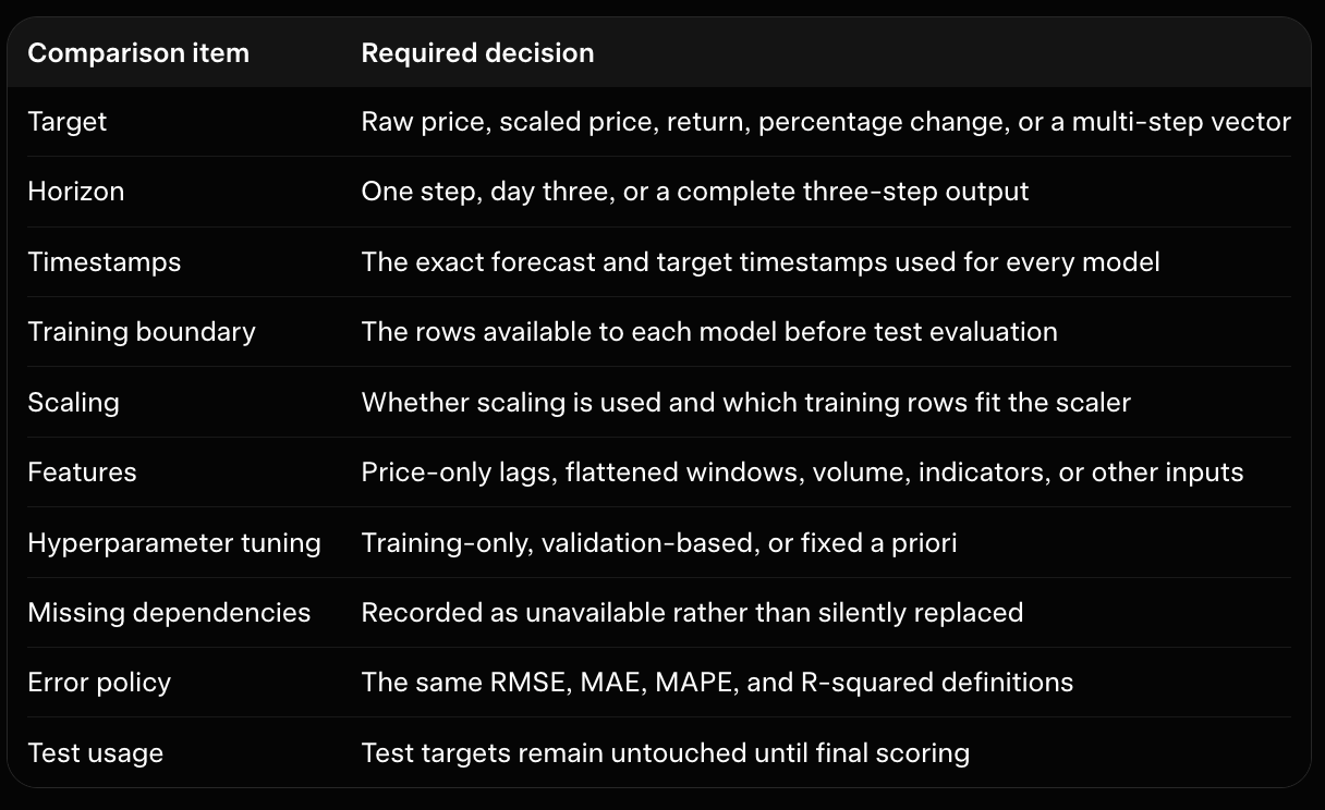
The generated run_benchmark_suite function attempts to provide one uniform workflow: extract training and test targets, fit each requested model on training data, predict the test interval, verify prediction length, calculate common metrics, and store implementation metadata. compare_forecasts then creates a stable pandas table and retains failed or unavailable models with status fields.

The common interface improves auditability, but it does not erase model-specific differences. An ARIMA model trained on a continuous series, an XGBoost model trained on flattened lag windows, and an HMM trained on price changes do not necessarily solve exactly the same statistical problem. Their input construction and forecast semantics must be described alongside their metric values.

10.9 Interpreting the paper's benchmark table

The paper reports Att-BiLSTM as the best listed predictor for both gold and Bitcoin. The extracted benchmark claims include values such as:

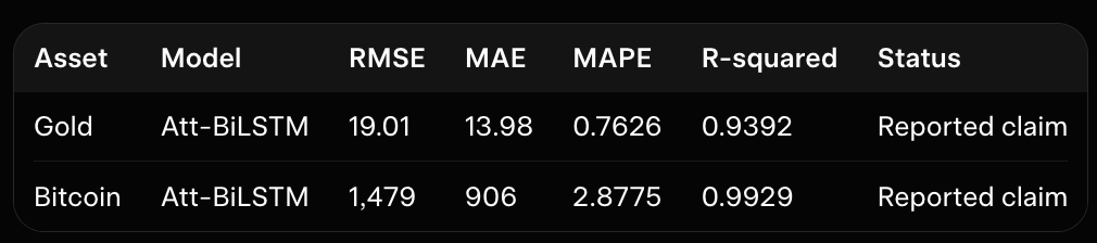
These numbers are preserved in the project documentation and reproduction matrix as unverified claims. They are not hard-coded acceptance targets for the benchmark adapters. The source data, preprocessing, architecture, hyperparameters, target scale, and test protocol are unavailable, so a different local experiment can legitimately produce different values without indicating a coding error.

The reproduction matrix makes this distinction explicit:

| Reported Att-BiLSTM gold metrics | Reported claim / Unavailable |
|---|---|
| RMSE 19.01, MAE 13.98, MAPE 0.7626, R-squared 0.9392 | Source data, preprocessing, target definition, and test protocol are missing. |

The same rule applies to the paper's LSTM, GRU, Holt-Winters, ARIMA, HMM, and XGBoost figures. A local comparison table can show what the supplied implementation produced under a documented protocol, but it cannot be called a reproduction of the paper's table until the missing inputs and decisions are recovered.

10.10 Forecast benchmarks are not trading benchmarks

Even a successful forecasting comparison is only one layer of the larger pipeline. The model with the lowest RMSE might not produce the best portfolio because:

• small forecast errors may not overcome transaction fees;

• the best numerical forecast may have poor directional timing;

• a position-sizing rule can amplify a modest error;

• different forecast horizons can produce different trading turnover;

• execution timing and slippage can reverse the order of model rankings;

• a high R-squared on a trending price level does not guarantee useful return forecasts.

For this reason, benchmark reporting should have two separate outputs:

Forecast comparison: target-level metrics using aligned test observations.

Trading comparison: portfolios generated from each model using the same signal, sizing, risk, fee, execution, and benchmark protocol.

The paper's reported Att-BiLSTM superiority addresses the first category as a claim. It does not, by itself, validate the second category.

10.11 Practical benchmark checklist

Before comparing local benchmark results, verify:

• Every model is trained only on its permitted training data.

• The final test targets are not used for model selection or hyperparameter tuning.

• All models forecast the same target representation and horizon, where comparison is intended.

• Forecast timestamps are aligned before calculating metrics.

• Price scaling is fitted on training data only and predictions are inverse-transformed consistently.

• MAPE near-zero behavior is documented.

• HMM state decoding is not mislabeled as a price forecast.

• XGBoost is described as gradient boosting, not random forest.

• Optional dependency failures remain visible in the results.

• Model-specific features and hyperparameters are recorded.

• Forecast metrics are reported separately from portfolio outcomes.

• Paper numbers are labeled as reported claims unless independently reproduced.

The generated benchmark adapters provide a useful scaffold for this process. Their main contribution is not a promise of identical numbers; it is a uniform, inspectable place to document how each alternative model was trained, what it predicted, whether it was available, and how its metrics were calculated.

11. Measure Returns and Consecutive Rise/Decline Streaks

The paper uses consecutive price increases and decreases to inform its position-management model. In practical terms, the analysis asks how often positive or negative price movements persist and how large representative gains and declines are.

The paper calls this procedure Apriori, but the extracted description does not define itemsets, support, confidence, or association rules. Standard Apriori is a frequent-itemset-mining algorithm, whereas the described procedure counts consecutive movements. The implementation therefore treats this component as streak analysis or sequential-pattern analysis. This is a terminology and implementation correction, not a claim that the paper's original authors intended a different method.

11.1 Define the return convention first

For adjacent prices, the standard simple return is:

\[ rt = \frac{pt-p{t-1}}{p{t-1}}. \]

The return is aligned with the later timestamp: it describes the move from the previous observation into p_t. For [100, 110, 99], the returns are:

100 -> 110: (110 - 100) / 100  =  0.10
110 ->  99: ( 99 - 110) / 110  = -0.10

The extracted paper equation appears to use the current price as the denominator:

\[ \tilde rt = \frac{pt-p{t-1}}{pt}. \]

Because the equation layout is ambiguous, compute_returns uses the conventional previous-price denominator by default and exposes the current-price form through an explicit option. The choice must be recorded and used consistently for classification, percentile estimation, sizing calibration, and any backtest signal.

The relevant implementation is in src/quantitative_trading_model/streaks.py:

def compute_returns(
    prices: Iterable[float],
    denominator: ReturnDenominator = "previous",
) -> np.ndarray:
    values = _as_float_array(prices, name="prices")
    if np.any(values <= 0.0):
        raise ValueError("prices must be strictly positive")

    if values.size < 2:
        return np.empty(0, dtype=float)

    normalized = str(denominator).lower()
    if normalized in {"previous", "previous_price"}:
        base = values[:-1]
    elif normalized in {"current", "current_price", "paper"}:
        base = values[1:]
    else:
        raise ValueError(
            "denominator must be 'previous', 'current', or 'paper'"
        )

    return (values[1:] - values[:-1]) / base

The function checks that prices are one-dimensional, finite, and strictly positive. A sequence with fewer than two prices has no adjacent return. Rejecting nonpositive prices is important because the return denominator would otherwise be invalid.

11.2 Classify rises, declines, and zero changes

Returns are classified numerically:

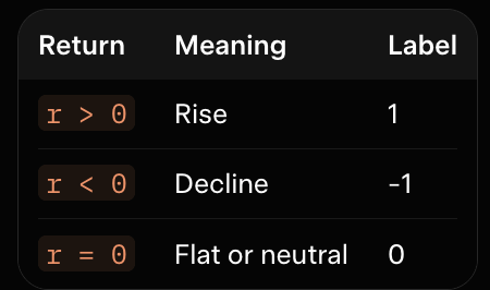
classify_returns returns integer labels, not strings such as "positive" or "neutral". Keeping the labels numeric makes run detection straightforward and avoids ambiguity in comparisons.

def classify_returns(
    returns: Iterable[float],
    *,
    zero_policy: ZeroPolicy = "neutral",
    tolerance: float = 0.0,
) -> np.ndarray:
    values = _as_float_array(returns, name="returns")
    labels = np.zeros(values.size, dtype=np.int8)
    labels[values > tolerance] = 1
    labels[values < -tolerance] = -1

    if zero_policy == "raise" and np.any(labels == 0):
        raise ValueError("zero or near-zero returns are not allowed")
    if zero_policy == "ignore":
        labels = labels[labels != 0]
    return labels

The zero policies are:

• neutral: retain zero labels, so they break maximal runs;

• terminate: treat zero changes as streak boundaries;

• ignore: remove zero labels before counting, making surrounding nonzero observations adjacent;

• raise: reject any zero or near-zero return.

The default is neutral. A nonzero tolerance can classify very small returns as zero; that setting should be included in experiment metadata because it changes the streak counts.

For example:

returns:  +   +   -   -   -   +   0   +
labels:    1   1  -1  -1  -1   1   0   1

Under the default policy, the zero separates the final positive movements. The positive runs have lengths two, one, and one, while the negative run has length three.

11.3 Maximal runs and overlapping subsequences

“Two consecutive rises” can refer to different statistics. The implementation supports both interpretations.

A maximal run is a complete uninterrupted sequence of one sign. For:

1, 1, -1, -1, -1, 1

the maximal runs are:

rise of length 2
decline of length 3
rise of length 1

The corresponding summaries are:

rise_streaks = {1: 1, 2: 1}
decline_streaks = {3: 1}

This answers: “How many complete runs of each exact length occurred?”

An overlapping subsequence count includes shorter patterns inside longer runs. A run of four rises contains three two-rise subsequences:

[1, 1] at positions 1-2
[1, 1] at positions 2-3
[1, 1] at positions 3-4

It also contains two three-rise subsequences and one four-rise subsequence. This answers: “How many contiguous patterns of each length occurred?”

The public function makes the distinction explicit:

def count_streaks(
    labels: Iterable[int],
    *,
    value: int,
    mode: StreakMode = "maximal",
    minimum_length: int = 1,
) -> dict[int, int]:
    result: dict[int, int] = {}
    run_length = 0

    for label in labels:
        if int(label) == value:
            run_length += 1
            continue

        if run_length:
            _add_run(
                result,
                run_length,
                mode=mode,
                minimum_length=minimum_length,
            )
            run_length = 0

    if run_length:
        _add_run(
            result,
            run_length,
            mode=mode,
            minimum_length=minimum_length,
        )
    return dict(sorted(result.items()))

The required value argument specifies whether to count rises (value=1) or declines (value=-1). In maximal mode, a run contributes one count for its exact length. In overlapping mode, a run of length r contributes r-j+1 occurrences for each subsequence length j.

The paper does not specify which counting convention it uses. Both are therefore implementation interpretations, not verified transcriptions. A research result should record the selected mode and minimum streak length.

11.4 Gain and decline percentiles

The paper connects streak analysis with percentile statistics used by its position-management method. The implementation keeps these quantities separate:

• the 90th percentile of positive returns;

• the 10th percentile of signed negative returns;

• the median positive return;

• the 10th percentile of positive decline magnitudes;

• the median decline magnitude.

For a negative return of -0.04, the signed decline is -0.04, while its magnitude is 0.04. Both forms are useful: the signed value preserves the return convention, and the magnitude is convenient for a sizing calculation that expects a nonnegative loss amount.

def estimate_gain_decline_percentiles(
    returns: Iterable[float],
    *,
    gain_percentile: float = 90.0,
    decline_percentile: float = 10.0,
) -> dict[str, float]:
    values = _as_float_array(returns, name="returns")
    gains = values[values > 0.0]
    declines = values[values < 0.0]
    decline_magnitudes = -declines

    return {
        "gain_percentile": _percentile(gains, gain_percentile),
        "decline_percentile": _percentile(
            declines, decline_percentile
        ),
        "gain_median": _percentile(gains, 50.0),
        "decline_magnitude_percentile": _percentile(
            decline_magnitudes, decline_percentile
        ),
        "decline_magnitude_median": _percentile(
            decline_magnitudes, 50.0
        ),
    }

For the return history:

[0.01, 0.02, 0.04, -0.01, -0.03, -0.06]

the gain sample is [0.01, 0.02, 0.04], and the signed decline sample is [-0.01, -0.03, -0.06]. The magnitude sample is [0.01, 0.03, 0.06]. Empty gain or decline samples produce NaN, rather than an invented zero.

These statistics are descriptive inputs to the later normalized exponential sizing reconstruction. They are not forecasts and do not imply that the next movement will match a historical percentile.

11.5 The combined summary record

compute_streak_statistics combines return calculation, classification, run counting, and percentile estimation. It returns a frozen StreakStatistics record containing the arrays, mappings, scalar statistics, denominator, zero policy, and streak mode.

“Frozen” means that the dataclass fields cannot be reassigned through normal dataclass operations. It does not make the stored NumPy arrays deeply immutable: a caller can still mutate an array in place unless it copies the arrays or marks them read-only. The record should therefore be treated as an audit-oriented summary object, not as a complete deep-immutability guarantee.

The returned record includes fields such as:

statistics = compute_streak_statistics(
    prices,
    denominator="previous",
    zero_policy="neutral",
    streak_mode="maximal",
)

print(statistics.rise_streaks)
print(statistics.decline_streaks)
print(statistics.gain_percentile_90)
print(statistics.decline_magnitude_percentile_10)

Its to_dict method is intended for local result files and preserves the selected conventions and count summaries.

11.6 Use only pre-decision information online

A full-history summary is useful for exploration but is not automatically valid for an out-of-sample strategy. If a signal is generated at time t, the statistics used to choose its position size must be estimated from returns known no later than t.

This is unsafe:

compute returns over the complete dataset
compute percentiles over the complete dataset
use those percentiles to size trades in the earlier test period

Future observations have influenced the historical calibration. The safer walk-forward pattern is:

for each decision timestamp t:
    use returns observed before t
    calculate or update streak statistics
    choose the next sizing level
    generate the order
    execute at a later permitted bar

The same rule applies when passing calibration statistics to build_exponential_schedule in sizing.py. A statistic calculated once from the entire dataset should not be used as though it had been available at every earlier decision time.

11.7 What the generated tests currently represent

tests/test_data_and_streaks.py is intended to document small, hand-calculable invariants such as the previous-price return convention and the difference between maximal and overlapping counts. However, the generated test file currently contains known API mismatches with the generated streaks.py implementation:

classify_returns returns integer labels 1, -1, and 0, while some test assertions expect textual labels such as "positive", "negative", and "neutral".

count_streaks requires the keyword-only value argument, but the generated streak-count test calls it without value=1 or value=-1.

These are planned/static test artifacts with known mismatches, not evidence of executable verification. They should be repaired before being treated as runnable tests: assertions should use numeric labels, and rise and decline counts should call count_streaks(labels, value=1, ...) and count_streaks(labels, value=-1, ...) separately.

Semantic code verification was skipped, and this tutorial does not claim that the tests were executed, that they pass, or that the paper's empirical results were reproduced. The useful review targets remain the return convention, zero policy, run-counting mode, percentile population, and pre-decision information boundary.

11.8 Summary

The paper's consecutive-movement component can be translated into an auditable pipeline:

Compute adjacent returns with an explicitly recorded denominator.

Classify each return as a rise, decline, or zero.

Decide how zero returns affect streak boundaries.

Count maximal runs or overlapping subsequences.

Estimate gain, signed-decline, and decline-magnitude percentiles.

Pass statistics to the later sizing reconstruction only when they could have been known at the decision timestamp.

The implementation in streaks.py provides these mechanics, but it does not claim to recover a standard Apriori algorithm or the paper's exact counting procedure. The appropriate description is sequential streak analysis feeding a documented, finite position-sizing reconstruction.

12. Reconstruct the Exponential Position-Sizing Rule Safely

The paper's position-management component addresses a different question from forecasting: after a strategy decides to trade, how much capital should it commit? The paper appears to increase later additions after successive declines, using empirical gains, declines, transaction costs, and an exponential sizing curve.

This section is not an exact reproduction of that method. The extracted forms of equations (5) through (8) contain damaged notation and do not define several important variables. The implementation in src/quantitative_trading_model/sizing.py therefore provides a finite, normalized-exponential alternative with explicit budget and exposure controls.

Reconstruction boundary: The schedule below is an auditable interpretation of the paper's sizing idea. It is not a faithful transcription of equations (5)–(8), and it does not establish that averaging down is safe or profitable.

12.1 Why the paper's recursive equations cannot be transcribed faithfully

The paper appears to derive later capital additions from a recovery or break-even condition: after one or more declines, a future gain should compensate for earlier losses and transaction costs. It then represents the resulting additions with an exponential curve.

The extracted equations are insufficient to reproduce that calculation reliably:

• p_i is not clearly defined as cash, asset quantity, or notional exposure.

• Signs and powers in the recursive expressions are corrupted.

• The fee convention is incomplete.

• The independent variable and exponent coefficient in the printed exponential expression are unclear.

• The maximum number of additions is not reliably specified.

• It is unclear whether an addition follows every observed decline, a forecast-confirmed decline, or a separate decision policy.

Those choices affect both risk and accounting. Filling them in silently would make the implementation appear more faithful than it is. The replacement below makes the missing decisions explicit.

12.2 Normalized exponential reconstruction

The practical reconstruction assigns a positive score to each finite addition level:

si=Aexp⁡(Bi),i=0,1,…,n−1.

Here A is a scale factor, B is the growth rate, and n is the configured maximum number of additions. The scores are converted to normalized weights:

\[ wi=\frac{si}{\sum{j=0}^{n-1}sj}. \]

For a sizing budget U, the planned allocation is:

\[ ai=Uwi. \]

Thus, subject to floating-point rounding,

\[ \sumi ai=U. \]

This is a plausible interpretation of the paper's normalized allocation expression, but it is not a verified transcription. In the generated implementation, build_exponential_schedule receives the number of additions and budget explicitly:

def build_exponential_schedule(
    max_additions: int,
    budget: float,
    *,
    growth: float = 0.5,
    amplitude: float = 1.0,
    gain_percentile: Optional[float] = None,
    decline_percentile: Optional[float] = None,
    fee_rate: float = 0.0,
    calibration_source: Any = None,
) -> SizingSchedule:
    """Build normalized ``A * exp(B*i)`` addition amounts."""

The absolute budget is therefore supplied to the sizing builder or sizer; it is not hidden inside the paper-inspired SizingConfig dataclass.

12.3 Constructing the schedule safely

The implementation computes the exponential scores and subtracts the largest exponent before calling exp:

indices = np.arange(max_additions, dtype=float)
exponents = growth * indices
exponents -= float(np.max(exponents))
scores_array = float(amplitude) * np.exp(exponents)

score_sum = float(scores_array.sum())
weights_array = scores_array / score_sum
allocations_array = weights_array * budget

Subtracting the maximum exponent does not change the normalized weights. It multiplies every score by the same positive constant, so each ratio s_i / sum(s_j) remains unchanged while reducing overflow risk.

SizingSchedule stores:

• scores: unnormalized exponential scores;

• weights: normalized proportions that sum to one; and

• allocations: planned currency amounts obtained from the budget.

It also records metadata identifying the formula as a reconstruction. This makes the sizing assumptions available when a later experiment is inspected.

12.4 Worked allocation example

Suppose the total planned budget is $1,000 and three levels have scores:

\[ s0=1, \qquad s1=2, \qquad s_2=4. \]

The score sum is 7:

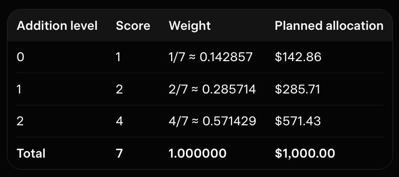
These are planned amounts, not automatic orders. If only $400 remains available when the final level is requested, the order must be reduced or rejected according to the current cash and exposure constraints.

The same relative scores arise from A=1 and B=log(2), because exp(Bi) then gives approximately 1, 2, and 4 for levels zero through two.

12.5 Optional percentile and fee calibration

The paper connects position sizing to empirical gain and decline statistics. The implementation can read values such as the 90th-percentile gain, a signed decline percentile, a decline-magnitude percentile, a median gain, and a fee rate.

When percentile values or a calibration_source are supplied to build_exponential_schedule, the helper _calibrated_growth derives a conservative growth coefficient:

def _calibrated_growth(
    gain_percentile: Optional[float],
    decline_percentile: Optional[float],
    fee_rate: float,
) -> tuple[float, dict[str, float]]:
    gain = max(float(gain_percentile or 0.0), 0.0)
    decline = abs(float(decline_percentile or 0.0))
    fee = _finite_nonnegative(fee_rate, "fee_rate")

    recovery = gain + _EPSILON
    burden = decline + 2.0 * fee
    growth = 0.05 + min(1.5, burden / recovery)
    return growth, {
        "gain_percentile": gain,
        "decline_magnitude": decline,
        "fee_rate": fee,
        "growth_coefficient": growth,
    }

This is an engineering interpretation, not the paper's recovered break-even equation. The fee appears twice in the burden term as a conservative allowance for a purchase and later sale; actual fees are still charged by the execution simulator.

SizingConfig contains fields such as calibrate_from_percentiles, recovery_percentile, decline_percentile, and fee_buffer. These fields document intended experiment settings, but the current generated schedule builder does not accept a SizingConfig directly and does not automatically consult calibrate_from_percentiles. Calibration is activated in the current implementation by supplying percentile arguments or a calibration_source to build_exponential_schedule. An experiment layer must explicitly connect configuration fields to those arguments if automatic configuration-driven calibration is desired.

12.6 Finite levels and budget invariants

The schedule validates finite values, nonnegative scores and allocations, normalized weights, and the relationship between planned allocations and its supplied budget. It also tracks consumed levels:

used_levels: set[int] = field(default_factory=set, repr=False)

next_unused_level() returns the first unconsumed level, and mark_used(level) records a level while rejecting reuse. This prevents a strategy loop from accidentally placing the same planned addition repeatedly.

The schedule's budget is an absolute amount supplied when the schedule is built. It is distinct from the fraction fields in SizingConfig. The configuration validates settings such as:

• a positive maximum_additions value;

• an initial_level inside the configured level range;

• a positive score_scale;

• allocation fractions between zero and one; and

• a maximum exposure fraction in (0, 1].

These checks validate fraction and level ranges. They do not compare an exposure fraction with an absolute budget, because SizingConfig does not contain an absolute budget field. Absolute budget and exposure constraints are enforced later by build_exponential_schedule and allocate_next_addition.

12.7 Cash and exposure caps at allocation time

The schedule is only a plan. At order time, allocate_next_addition applies the current portfolio state:

def allocate_next_addition(
    schedule: SizingSchedule,
    available_cash: float,
    *,
    current_exposure: float = 0.0,
    max_exposure: Optional[float] = None,
    level: Optional[int] = None,
    allow_partial: bool = True,
) -> AllocationDecision:

The effective capacity is calculated as:

cap = schedule.budget if max_exposure is None else max_exposure
capacity = min(cash, max(0.0, cap - exposure))
approved = min(requested, capacity)

This provides three separate protections:

A request cannot exceed current available cash.

Available cash does not override a maximum exposure limit.

Partial approval is explicit. With allow_partial=True, an amount may be reduced to capacity; with allow_partial=False, an undersized request is rejected.

The result is an AllocationDecision containing the requested and approved amounts, selected level, reason, remaining cash, and remaining exposure capacity.

The approved amount is a pre-fee notional. The sizing module does not deduct execution fees from that amount. The backtest applies fees separately, so the final cash cost of a buy can be higher than the approved notional. Consequently, the execution layer may clip the order again when fees are applied, even when the sizing layer approved it under a pre-fee cash calculation. Keeping these stages separate makes the fee convention auditable, but callers must not treat a pre-fee approval as a guarantee that the full order will fill.

12.8 Why this is not unlimited averaging down

Increasing allocations after declines can become an uncontrolled averaging-down strategy. The generated design limits that behavior by using:

• a finite maximum_additions value;

• one-time consumption of each addition level;

• a fixed schedule budget;

• current-cash checks;

• optional maximum exposure;

• no leverage by default in the execution layer; and

• optional risk filtering by later strategy components.

These are safety and reproducibility choices, not recovered paper details. They may differ from the unknown original behavior, but they prevent the implementation from silently authorizing unlimited purchases.

The sizing module also does not decide when to add. It supplies an amount after another layer requests a level. A signal, forecast, decline condition, VaR decision, or greedy policy must determine whether that level is activated.

12.9 Correct API example

The generated sizing implementation uses growth, not growth_rate, when constructing a schedule:

schedule = build_exponential_schedule(
    budget=1_000.0,
    max_additions=4,
    growth=0.5,
)

assert np.isclose(sum(schedule.weights), 1.0)
assert np.isclose(sum(schedule.allocations), 1_000.0)

The supplied generated test file uses growth_rate in one example and constructs ExponentialPositionSizer with a configuration object in a way that does not match the shown implementation. It also contains related naming differences in the risk and strategy tests. These are static test artifacts describing intended invariants, not evidence that the tests were executed successfully. The corrected example above follows the actual generated build_exponential_schedule signature.

12.10 What the sizing tests are intended to verify

The tests are intended to check properties of the reconstruction rather than the paper's unverified returns:

• scores, weights, and allocations are finite;

• weights are nonnegative and sum to one;

• planned allocations do not exceed the supplied budget;

• a request cannot exceed available cash or exposure capacity;

• an addition level cannot be reused; and

• future realized prices do not influence the sizing decision.

These are static and semantic expectations. They do not prove that equations (5)–(8) were recovered or that the resulting strategy is economically sound.

12.11 Practical interpretation

The reconstructed data flow is:

historical gain/decline statistics
        |
        v
optional explicit calibration arguments
        |
        v
finite exponential scores
        |
        v
normalized budget allocations
        |
        v
cash and exposure checks
        |
        v
pre-fee approved notional
        |
        v
fee-aware execution and final fill

A larger allocation after a decline increases potential exposure if prices recover, but it also increases losses if the decline continues. Fees, slippage, liquidity, and forecast error can invalidate the recovery assumptions. Evaluation should therefore include drawdown, turnover, total fees, and risk measures rather than final value alone.

The narrow claim supported by this implementation is that it provides a finite, normalized, auditable reconstruction of the paper's exponential position-sizing concept. It does not reproduce equations (5)–(8), validate the paper's reported $646 gold or $215,487 Bitcoin outcomes, or establish profitability.

13. Turn Forecasts into Signals and Reconstruct the Greedy Policy

A forecast is not yet an order. If a model predicts Bitcoin will reach $31,000, the strategy must still compare that prediction with the current price, decide whether the expected move is large enough to trade, choose a notional amount, check cash and exposure limits, apply risk controls, and select an action.

The paper describes this stage using forecasting, position management, risk control, and a modified greedy algorithm. It does not define the greedy algorithm operationally: the candidate actions, objective, constraints, and tie-breaking rules are missing. The implementation therefore provides a transparent reconstructed policy, not a verified reproduction.

The intended decision flow is:

forecast values
    -> aggregate the forecast horizon
    -> compare the forecast with the current price
    -> create a buy, sell, add, or hold signal
    -> construct and constrain candidate actions
    -> estimate fees and expected benefit
    -> apply a risk filter
    -> rank feasible candidates deterministically
    -> execute the selected action on a later bar

The snippets in this section are abridged explanatory excerpts from src/quantitative_trading_model/strategy.py; they are not complete replacement functions. The generated strategy and risk modules currently have an incompatible runtime interface, so this section describes the intended contract and the required repair rather than claiming that the end-to-end policy runs successfully.

13.1 Direction and order size are separate decisions

The strategy module defines four directional states:

class Signal(str, Enum):
    BUY = "buy"
    SELL = "sell"
    HOLD = "hold"
    ADD = "add"

These values describe intent, not quantity:

• BUY establishes or increases exposure when the forecast exceeds a threshold.

• SELL reduces existing long exposure when the forecast is sufficiently negative.

• ADD requests the next finite position-sizing level.

• HOLD submits no trade.

Separating direction from size lets the forecasting model answer “should an opportunity be considered?” while the sizing module answers “how much may be allocated?” Cash limits, exposure caps, transaction fees, and risk controls can then reduce or reject the proposed amount.

The paper does not explain how an ADD signal is triggered. In particular, it does not state whether additions follow every decline, a forecast-confirmed decline, or a separate greedy rule. The generated strategy.py does not derive ADD directly from the streak analysis; it creates an addition candidate only when the supplied decision is BUY or ADD and a finite addition level is available. A production revision must define that trigger explicitly.

13.2 Aggregate one-day or multi-day forecasts explicitly

The paper is inconsistent about its forecast horizon. Its prediction discussion supports one-step forecasting, while its conclusion refers to the next three days. SignalGenerator makes the interpretation configurable.

The generator accepts predicted prices and supports three aggregation choices:

• terminal: use the final forecast, such as day three;

• mean: use the average forecast over the horizon;

• max: use the largest forecast.

The following is an abridged excerpt; validation and error handling remain in the generated class:

class SignalGenerator:
    def __init__(self, buy_threshold=0.0, sell_threshold=0.0,
                 aggregation="terminal", minimum_forecast_points=1):
        self.buy_threshold = buy_threshold
        self.sell_threshold = sell_threshold
        self.aggregation = aggregation
        self.minimum_forecast_points = minimum_forecast_points

    def aggregate(self, forecasts):
        values = [float(value) for value in forecasts]
        if self.aggregation == "terminal":
            return values[-1]
        if self.aggregation == "mean":
            return sum(values) / len(values)
        return max(values)

For a current price of $100 and forecasts [101, 103, 104], terminal and maximum aggregation produce $104, while mean aggregation produces approximately $102.67. These are reconstruction choices, not rules confirmed by the paper.

13.3 Convert the selected forecast into a signal

After aggregation, the strategy computes the expected price return:

r^=p^−pp,

where p is the current price and p_hat is the selected forecast.

An abridged version of SignalGenerator.decide is:

def decide(self, current_price, forecasts):
    forecast_value = self.aggregate(forecasts)
    expected_return = forecast_value / current_price - 1.0

    if expected_return > self.buy_threshold:
        signal = Signal.BUY
    elif expected_return < -self.sell_threshold:
        signal = Signal.SELL
    else:
        signal = Signal.HOLD

    return SignalDecision(
        signal=signal,
        expected_return=expected_return,
        forecast_value=forecast_value,
        horizon=len(forecasts),
        rationale="threshold-based forecast decision",
    )

With one-percent buy and sell thresholds:

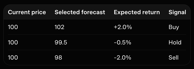
The thresholds are not specified by the paper and must be stored with experiment metadata. A zero threshold can produce frequent trades when forecasts fluctuate around the current price; a positive threshold creates a hold band but may delay decisions.

A signal must contain current-information fields only: direction, expected return, forecast value, horizon, and rationale. It must not contain a realized future price or realized future return. Execution belongs to the later backtest stage.

13.4 Candidate actions contain size and audit information

A CandidateAction combines a proposed notional with the information needed for ranking:

@dataclass(frozen=True)
class CandidateAction:
    signal: Signal
    notional: float              # pre-fee order value
    expected_return: float
    estimated_fee: float
    score: float
    feasible: bool = True
    reason: str = ""
    addition_level: Optional[int] = None
    risk_approved: bool = True
    risk_scale: float = 1.0

For buys and additions, notional is the cash committed before fees. For sells, it is the market value sold before the sell fee. reason and addition_level make decisions easier to inspect.

PortfolioSnapshot supplies the current state:

@dataclass(frozen=True)
class PortfolioSnapshot:
    cash: float
    holdings: float
    price: float
    addition_level: int = 0
    portfolio_value: Optional[float] = None
    max_exposure: Optional[float] = None

    @property
    def marked_value(self):
        return self.cash + self.holdings * self.price

This state is intentionally limited to information available at the signal timestamp.

13.5 Apply feasibility constraints before ranking

The policy should never rank an unaffordable order as though it were executable. For a long-only account, the main constraints are:

A buy must fit available cash, including fees.

A buy must not exceed the maximum exposure.

A sell must not exceed current holdings unless shorting is explicitly enabled.

An addition must use an available finite sizing level.

A risk filter may subsequently block or scale the candidate.

For a fee rate f, the maximum pre-fee buy notional from cash is:

Nmax=cash1+f.

Thus $75 of cash and a one-percent fee permit at most approximately $74.26 of pre-fee buy notional.

The generated candidate builder caps buy amounts by cash and exposure. It does not consistently retain a separate rejected candidate for every failed cash or exposure check. Some rejected requests are reduced to an affordable candidate, while exhausted addition levels may be recorded as infeasible. Therefore, the accurate audit statement is that feasible capped candidates and selected/rejected addition cases are recorded, but the current implementation does not provide a uniform record of every failed constraint attempt. A stricter audit design would preserve both the original request and the resulting rejection reason.

A conceptual candidate calculation is:

available_buy = snapshot.cash / (1.0 + fee_rate)
current_exposure = snapshot.holdings * snapshot.price

if snapshot.max_exposure is not None:
    available_buy = min(
        available_buy,
        max(0.0, snapshot.max_exposure - current_exposure),
    )

The backtest must enforce the same limits again at execution. Strategy-level feasibility is not a substitute for accounting-level validation.

13.6 Connect finite sizing to ADD candidates

The normalized exponential sizer supplies finite addition amounts. The strategy layer should not duplicate the sizing formula. It requests the next level from a previously constructed sizer or schedule, then applies current cash and exposure limits.

For example, the sizing object must be defined before calling the policy:

from quantitative_trading_model.sizing import (
    ExponentialPositionSizer,
    build_exponential_schedule,
)

schedule = build_exponential_schedule(
    max_additions=3,
    budget=500.0,
    growth=0.5,
)
sizer = ExponentialPositionSizer(schedule=schedule)

The exact generated API may need alignment before runtime use, but the intended data flow is:

BUY or ADD decision
    -> request the next sizing level
    -> cap it by cash and exposure
    -> create an ADD candidate

The paper does not define the trigger for ADD, so the example must not imply that the strategy automatically reacts to every consecutive decline. That behavior would need an explicit rule connecting streaks.py, the forecast, and the policy.

13.7 Use a transparent fee-aware score

The paper gives no objective function for its modified greedy algorithm. The reconstruction uses expected net benefit:

score(a)=notional(a)(benefit rate(a)−f).

For a buy or add, the benefit rate is the forecasted return. For a sell, the reconstruction treats a negative forecast as a potential avoided loss, so the benefit rate is -expected_return. Hold has a score of zero.

An abridged scoring function is:

def score_candidate_action(action, *, expected_return, fee_rate):
    if action.signal in {Signal.BUY, Signal.ADD}:
        benefit_rate = expected_return
    elif action.signal is Signal.SELL:
        benefit_rate = -expected_return
    else:
        benefit_rate = 0.0
    return action.notional * (benefit_rate - fee_rate)

A $100 buy with a three-percent expected return and one-percent fee scores:

100(0.03−0.01)=2.

A $100 buy with a 0.5% expected return scores -0.50 and should lose to the zero-score hold action. This score ignores uncertainty, spread, liquidity, and forecast calibration. It is a transparent replacement for an objective that the paper does not provide.

13.8 Rank candidates deterministically

The intended ranking process is:

Remove candidates that are infeasible or not risk-approved.

Choose the highest score.

Break equal-score ties with the smaller notional.

Apply a fixed signal priority for any remaining tie.

An abridged selection expression is:

feasible = [
    candidate for candidate in candidates
    if candidate.feasible and candidate.risk_approved
]

selected = max(
    feasible,
    key=lambda candidate: (
        candidate.score,
        -candidate.notional,
        -priority[candidate.signal],
    ),
)

The priority mapping is an implementation choice, not a paper rule. If no candidate is feasible, the policy should return a hold decision with a clear reason such as "no feasible candidate".

13.9 Risk integration: intended contract versus current generated code

The intended ordering is:

candidate
    -> risk filter
    -> accept, scale, or block
    -> recompute fee and score
    -> rank the resulting candidate

Risk must be applied before final ranking because scaling a candidate can change its score. However, the current generated strategy.py and risk.py do not implement one reliable shared protocol:

• GreedyPolicy._apply_risk calls the filter using proposed_notional, while VaRTradeFilter.decide expects proposed_quantity and also requires current_exposure and portfolio_value.

• The fallback positional call does not reliably map those required values to the risk method's parameters.

• VaRTradeFilter returns RiskDecision with approved_quantity and blocked, not an approved field. The current strategy adapter looks first for approved or allowed, so a blocked result can be misinterpreted as approved.

• Consequently, the current code must be repaired before its VaR integration can be treated as a working runtime policy.

A strict repaired protocol should pass the same named fields every time:

risk_decision = risk_filter.decide(
    proposed_quantity=action.notional,
    current_exposure=snapshot.holdings * snapshot.price,
    portfolio_value=snapshot.value,
    returns=pre_decision_returns,
)

if risk_decision.blocked:
    action = replace(action, feasible=False, risk_approved=False, notional=0.0)
elif risk_decision.approved_quantity < action.notional:
    scale = risk_decision.approved_quantity / action.notional
    action = rescale_and_recompute_score(action, scale, fee_rate)

This is a repair specification, not a claim about the current generated files. The paper itself does not define how VaR interacts with greedy selection, so the ordering remains a reconstruction even after the interfaces are aligned.

13.10 Complete decision example with explicit assumptions

The following is an explanatory excerpt showing the objects that must exist. It is not a complete runnable example, and the risk interface must be repaired as described above:

from quantitative_trading_model.strategy import (
    GreedyPolicy, PortfolioSnapshot, SignalGenerator,
)

schedule = build_exponential_schedule(
    max_additions=3,
    budget=500.0,
    growth=0.5,
)
sizer = ExponentialPositionSizer(schedule=schedule)

policy = GreedyPolicy(fee_rate=0.01)
signal_generator = SignalGenerator(
    buy_threshold=0.01,
    sell_threshold=0.01,
    aggregation="terminal",
)

snapshot = PortfolioSnapshot(
    cash=500.0,
    holdings=0.0,
    price=100.0,
    addition_level=0,
    max_exposure=500.0,
)

# The intended call; risk_filter integration requires the strict protocol above.
action = policy.choose(
    snapshot,
    forecasts=[101.0, 103.0, 104.0],
    signal_generator=signal_generator,
    sizer=sizer,
    max_additions=3,
)

Conceptually, this selects the terminal forecast of $104, computes a four-percent expected return, creates a buy decision, obtains finite sizing candidates, applies cash and exposure limits, accounts for fees, and selects the best feasible action. The selected action must be passed to the backtest for execution on a later bar.

13.11 Verification status and no-look-ahead boundary

The intended tests in tests/test_sizing_risk_strategy.py cover useful invariants:

• scores use forecasts and fees rather than realized future returns;

• order sizes do not exceed cash or exposure limits;

• risk scaling never increases a proposed order;

• tie-breaking is deterministic;

• signal timestamps precede execution timestamps.

The supplied generated test file is currently API-inconsistent with strategy.py. It uses older names such as side instead of signal and calls methods with incompatible signatures. It therefore cannot substantiate that the current strategy implementation passes its intended tests without repair.

More broadly, semantic code verification was skipped. Static review identified issues in the generated project, and no code execution or passing test suite is being claimed. The excerpts above explain the intended contracts and invariants; they should not be read as evidence of runtime correctness.

13.12 Reproduction boundary

The paper's greedy policy remains unverified because it does not specify:

• the complete candidate-action set;

• whether one action or a multi-step plan is selected;

• the objective function;

• how one-day and three-day forecasts are combined;

• the treatment of fees, spreads, and slippage;

• the interaction between VaR and action selection;

• leverage, exposure, and addition constraints; or

• tie-breaking behavior.

The generated policy is therefore best understood as an auditable baseline. It demonstrates how forecasts, finite sizing, constraints, fees, risk decisions, and deterministic selection can be connected without using realized future prices. The realized price enters only during later execution and evaluation, preserving the causal boundary required for a meaningful backtest.

14. Add Historical VaR as an Explicit Risk Filter

The paper names Value-at-Risk (VaR) as part of its trading framework, but it does not define the parameters or the action taken when risk is high. It does not specify the confidence level, horizon, lookback window, return distribution, portfolio aggregation, acceptable loss, or whether VaR blocks or scales trades.

This project therefore uses a rolling historical VaR reconstruction. The convention in this section is explicit:

• return VaR is a nonnegative loss fraction, such as 0.04 for a 4% loss threshold;

• projected VaR is a currency amount;

• the risk limit is a currency amount equal to a configured fraction of portfolio value;

• trades may be accepted, scaled, or blocked;

• only returns available before the decision timestamp may be used.

These choices are operational assumptions, not a verified implementation of the paper's VaR method.

14.1 VaR sign convention and units

Let r be a collection of historical returns and let alpha be the confidence level. The lower-tail return quantile is q_(1-alpha)(r). A positive return-loss VaR is:

\[ \operatorname{VaR}^{\text{return}}\alpha = -q{1-\alpha}(r). \]

If the 5th-percentile return at 95% confidence is -0.04, return VaR is 0.04.

For an exposure E, projected currency VaR is:

\[ \operatorname{VaR}^{\text{currency}}\alpha = E\times \operatorname{VaR}^{\text{return}}\alpha. \]

For example, a $2,000 exposure and a 4% return-loss VaR produce:

projected currency VaR = 2,000 * 0.04 = $80

The units are important. A currency VaR must be compared with a currency limit, not with a fraction such as 0.05.

The risk limit is calculated from portfolio value V and the configured maximum fraction m:

limitcurrency=mV.

Thus, for a $10,000 portfolio and m=0.05, the limit is $500.

VaR is a loss quantile, not a guaranteed maximum loss. A realized loss can exceed it, particularly when market conditions change or the historical window does not represent the current regime.

14.2 Explicit configuration

VaRConfig in src/quantitative_trading_model/config.py makes the unspecified choices visible:

@dataclass
class VaRConfig:
    enabled: bool = True
    confidence: float = 0.95
    horizon: int = 1
    lookback: int = 100
    method: str = "historical"
    action: str = "scale"
    max_var_fraction: float = 0.05
    insufficient_history: str = "allow"
    min_observations: int = 30

The defaults are implementation choices:

| Setting | Default | Meaning | | --- | ---: | --- | | confidence | 0.95 | Use the lower 5% return tail. | | horizon | 1 | Estimate a one-period loss threshold. | | lookback | 100 | Use at most the latest 100 available returns. | | method | historical | Use an empirical quantile. | | action | scale | Reduce an order that exceeds the risk limit. | | max_var_fraction | 0.05 | Permit VaR up to 5% of portfolio value. | | min_observations | 30 | Require this many horizon observations for an actionable estimate. |

Configuration validation rejects invalid confidence levels, nonpositive horizons and lookbacks, unsupported methods, and unknown action modes. Decimal transaction fees, forecast settings, sizing settings, and execution rules remain separate from VaR.

14.3 Estimating a rolling historical quantile

HistoricalVaR in src/quantitative_trading_model/risk.py performs the following steps:

Convert the supplied returns to a finite one-dimensional array.

Keep only the configured lookback window.

Optionally construct overlapping compounded returns for a multi-period horizon.

Select the lower-tail empirical quantile.

Store the signed quantile and its nonnegative loss magnitude.

The central calculation is:

values = self._finite_returns(returns)
values = values[-self.lookback:]
horizon_values = self._horizon_returns(values)

if len(horizon_values) < self.min_observations:
    return VaREstimate(
        var=float("nan"),
        confidence=self.confidence,
        horizon=self.horizon,
        observations=len(horizon_values),
        return_quantile=float("nan"),
        sufficient_history=False,
    )

quantile = np.quantile(
    horizon_values,
    1.0 - self.confidence,
    method="linear",
)
return VaREstimate(
    var=max(0.0, -float(quantile)),
    confidence=self.confidence,
    horizon=self.horizon,
    observations=len(horizon_values),
    return_quantile=float(quantile),
    sufficient_history=True,
)

VaREstimate.var is a return fraction. It is not a currency amount until it is multiplied by an exposure. return_quantile retains the signed empirical value for auditing.

The 1-confidence probability is deliberate. With confidence=0.95, the implementation selects the 5th percentile. The sign conversion prevents a negative return quantile from being confused with a negative risk amount.

14.4 Optional horizon compounding

For a one-period horizon, the historical returns can be used directly. For a longer horizon, consecutive simple returns are compounded. A two-period return is:

\[ (1+rt)(1+r{t+1})-1. \]

The corresponding helper is:

def _horizon_returns(self, values: np.ndarray) -> np.ndarray:
    if self.horizon == 1:
        return values
    if values.size < self.horizon:
        return np.empty(0, dtype=float)

    windows = np.lib.stride_tricks.sliding_window_view(
        values,
        self.horizon,
    )
    return np.prod(1.0 + windows, axis=1) - 1.0

Overlapping historical blocks are a transparent reconstruction. The paper does not say whether its VaR uses one-day returns, compounded multi-day returns, a parametric distribution, or simulation.

14.5 Pre-decision history and lookback boundaries

VaR must obey the same information boundary as the forecast. If a decision is made after observations through time t, the risk history may contain returns known by that point, but not returns from t+1 or later.

HistoricalVaR accepts caller-supplied returns and cannot infer timestamps. The caller is responsible for constructing the correct information set:

# known_returns must contain only returns available at the signal time
estimate = var_estimator.estimate(known_returns, include_last=True)

If the final element represents a current-bar return that is not yet available when the signal is formed, use include_last=False:

estimate = var_estimator.estimate(
    known_returns,
    include_last=False,
)

A leakage-aware sequence is:

1. Observe prices through the information timestamp.
2. Compute only returns available at that timestamp.
3. Estimate VaR from the permitted lookback window.
4. Generate the forecast and candidate order.
5. Apply the VaR filter.
6. Execute no earlier than the next permitted bar.

The risk module must not be passed the complete historical return series during every past decision. That would use future information.

14.6 Insufficient history

When fewer than min_observations horizon returns are available, HistoricalVaR.estimate returns an estimate with sufficient_history=False and unavailable numerical values. It does not fabricate a zero-risk estimate.

VaRTradeFilter then applies the configured policy:

• insufficient_history="allow" permits the order while recording that VaR was unavailable;

• insufficient_history="block" rejects positive buy exposure until enough history exists.

This is a policy choice that belongs in experiment metadata. Missing risk information is not evidence that risk is zero.

14.7 Projecting VaR consistently in currency units

The corrected unit contract for the risk filter is:

def projected_var(
    self,
    estimate: VaREstimate,
    *,
    exposure: float,
    portfolio_value: float,
) -> float:
    """Return projected VaR as a currency amount."""
    if not estimate.sufficient_history:
        return float("nan")
    if portfolio_value <= 0:
        raise ValueError("portfolio_value must be positive")
    if exposure < 0:
        raise ValueError("exposure must be nonnegative")
    return estimate.var * exposure

The portfolio value is needed for the limit, not for dividing the projected loss:

limit = self.max_var_fraction * portfolio_value
projected = self.projected_var(
    estimate,
    exposure=projected_exposure,
    portfolio_value=portfolio_value,
)

For a 4% return VaR and $2,000 exposure, projected_var returns $80. For a $10,000 portfolio and a 5% limit, the comparison is $80 <= $500; both sides are currency amounts.

This avoids mixing a portfolio-relative fraction with a currency limit. If a project instead chooses to return a relative fraction, it must compare that result with max_var_fraction directly. The implementation described here uses currency amounts throughout the decision path.

14.8 Accept, scale, and block behavior

VaRTradeFilter applies a risk decision to a proposed notional quantity. Its modes are:

Accept

Approve the proposed quantity. This can be used when VaR is informational or when the order is already within the limit.

Block

Return an approved quantity of zero when projected currency VaR exceeds the currency limit.

Scale

Approve the largest quantity that remains within the limit. With portfolio value V, limit fraction m, and return VaR v, the maximum total exposure is:

Emax=mVv,

provided v > 0. The maximum additional buy is this amount minus current exposure.

A consistent decision core is:

limit = self.max_var_fraction * portfolio_value
buy_amount = max(proposed_quantity, 0.0)
full_exposure = current_exposure + buy_amount
full_var = self.projected_var(
    estimate,
    exposure=full_exposure,
    portfolio_value=portfolio_value,
)

if proposed_quantity <= 0 or full_var <= limit:
    return RiskDecision(
        "accept",
        proposed_quantity,
        proposed_quantity,
        1.0,
        full_var,
        limit,
        current_exposure,
        full_exposure,
        "within VaR limit or exposure-reducing order",
        True,
    )

if self.action == "block" or estimate.var <= 0:
    return RiskDecision(
        "block",
        proposed_quantity,
        0.0,
        0.0,
        full_var,
        limit,
        current_exposure,
        current_exposure,
        "proposed exposure exceeds VaR limit",
        True,
    )

allowed_exposure = limit / estimate.var
allowed_buy = max(0.0, allowed_exposure - current_exposure)
approved = min(proposed_quantity, allowed_buy)
scale = approved / proposed_quantity if proposed_quantity else 0.0

The critical correction is allowed_exposure = limit / estimate.var, not limit * portfolio_value / estimate.var, because limit is already a currency amount. Similarly, projected_var returns estimate.var * exposure, not estimate.var * exposure / portfolio_value.

14.9 Connecting VaR to the strategy layer

The strategy flow is:

forecast
  -> signal
  -> candidate notional
  -> cash and exposure checks
  -> VaR accept / scale / block
  -> greedy ranking
  -> next-bar execution

The VaR call must use the same argument names and units as VaRTradeFilter.decide. In particular, GreedyPolicy should pass the proposed order as proposed_quantity, current marked exposure as current_exposure, and portfolio value as portfolio_value:

risk_decision = self.risk_filter.decide(
    proposed_quantity=action.notional,
    current_exposure=snapshot.holdings * snapshot.price,
    portfolio_value=snapshot.value,
    returns=returns,
)

The selected quantity is then taken from risk_decision.approved_quantity. A blocked action must be marked infeasible, and a scaled action must be rescored using its approved notional before greedy ranking. The risk filter must never increase the proposed quantity.

This explicit adapter is preferable to relying on incompatible keyword aliases such as proposed_notional when the risk API requires proposed_quantity. The strategy and risk modules should share one documented contract rather than silently catching argument errors.

14.10 Treatment of sells

The default filter is a long-exposure filter. A negative proposed quantity represents a sell. A sell that reduces long exposure is accepted by this filter because it does not increase the projected long exposure.

This does not constitute a complete portfolio-risk model. It does not model short positions, leverage, cross-asset correlations, liquidity, spread, market impact, or nonlinear instruments. The paper's brief mention of VaR does not justify assuming those features.

14.11 Numerical examples

Suppose:

portfolio value       = $10,000
current exposure       = $2,000
proposed buy           = $3,000
return VaR             = 4%
maximum VaR fraction   = 5%

The complete proposed exposure is $5,000, so projected currency VaR is:

$5,000 * 0.04 = $200

The currency limit is:

$10,000 * 0.05 = $500

Because $200 <= $500, the VaR layer accepts the proposed order, subject to cash, sizing, fee, and exposure constraints elsewhere.

If return VaR is 12% instead:

full projected VaR = $5,000 * 0.12 = $600
risk limit         = $500

In scale mode, maximum total exposure is:

$500 / 0.12 = approximately $4,166.67

After subtracting the existing $2,000 exposure, the maximum additional buy is approximately $2,166.67. In block mode, the $3,000 proposed order is rejected.

These examples describe the reconstructed unit-consistent policy. They do not establish what the paper's original VaR procedure did.

14.12 Tests and verification boundary

Tests for the corrected API should call the actual interfaces directly. For example:

var = HistoricalVaR(
    confidence=0.95,
    horizon=1,
    lookback=len(returns),
    min_observations=2,
)
estimate = var.estimate(returns)

risk_filter = VaRTradeFilter(
    var_estimator=var,
    max_var_fraction=0.005,
    action="block",
)
decision = risk_filter.decide(
    proposed_quantity=500.0,
    current_exposure=0.0,
    portfolio_value=1_000.0,
    estimate=estimate,
)

assert decision.approved_quantity <= 500.0

The test should not pass portfolio_value to HistoricalVaR.estimate, because historical estimation uses returns and VaR configuration; portfolio value belongs to exposure projection and trade filtering. It should also use max_var_fraction, not an unsupported max_var constructor argument, and should call decide with proposed_quantity, current_exposure, and portfolio_value.

These are invariant-level checks, not empirical validation. Static and semantic review can inspect units, argument contracts, and no-look-ahead behavior, but no claim is made here that the generated code was executed. The supplied verification record states that semantic code verification was skipped, so the risk tests and integration snippets should be treated as corrected intended contracts until the source artifacts are aligned and independently checked.

14.13 Reproducibility boundary

This VaR layer remains reconstructed. A verified implementation of the paper would require at least:

the confidence level;

the VaR horizon;

the return definition and portfolio aggregation method;

the estimation window;

the historical or parametric estimation method;

the maximum acceptable loss or exposure threshold;

whether VaR blocks, scales, or merely reports trades;

how VaR interacts with the greedy policy and position-sizing schedule.

The accurate claim is therefore: the project defines a documented rolling historical VaR filter with consistent currency units and explicit action rules, inspired by the paper's risk-control description. It does not claim to reproduce the paper's unspecified VaR method or its reported investment outcomes.

15. Simulate Next-Bar Execution and Portfolio Accounting

A forecast becomes useful to a backtest only after it is converted into an order and accounted for consistently. The paper describes a combined trading framework, but it does not fully specify signal timing, execution prices, fee conventions, slippage, liquidation, or portfolio accounting. The generated implementation therefore makes these choices explicit in src/quantitative_trading_model/backtest.py.

These rules are reconstructions, not claims about the paper's exact backtest. The simulator is offline: it accepts caller-supplied local prices and orders and does not connect to an exchange or submit live orders.

15.1 Signal time and execution time

A strategy forms a signal using information available at time t. The order must execute at a later timestamp. The simulator enforces that ordering:

historical window ends at t
    -> forecast and signal are generated at t
    -> order is submitted for a later bar
    -> fill occurs after t
    -> portfolio is marked to market

The Order dataclass records both the signal and intended execution timestamps:

@dataclass(frozen=True)
class Order:
    side: str
    quantity: float | None = None
    signal_timestamp: Any = None
    execution_timestamp: Any = None
    notional: float | None = None
    addition_level: int | None = None
    reason: str = ""
    metadata: Mapping[str, Any] = field(default_factory=dict)

An order may specify asset units through quantity or a currency amount through notional. In the current implementation, a notional order is converted to units using the supplied reference price before slippage is applied. Therefore, with nonzero slippage, the executed notional can differ from the requested notional. This is an implementation detail that should be recorded in experiment metadata rather than described as conversion at the final slippage-adjusted price.

PortfolioSimulator.execute rejects same-bar and earlier execution:

fill_time = _timestamp(timestamp)
signal_time = _timestamp(order.signal_timestamp)
if fill_time <= signal_time:
    raise ValueError(
        "Orders must execute strictly after their signal timestamp"
    )

This prevents a signal generated from a closing price from being filled at that same closing price. The simulator enforces a later timestamp, but it does not independently determine that the timestamp is exactly the next bar. A caller must supply next-bar orders or use a scheduling layer that does so.

Each completed order becomes a Fill record containing its timing and accounting details:

@dataclass(frozen=True)
class Fill:
    timestamp: Timestamp
    signal_timestamp: Timestamp
    side: str
    quantity: float
    reference_price: float
    execution_price: float
    notional: float
    fee: float
    cash_change: float
    reason: str = ""
    addition_level: int | None = None

Thus, a fill is an auditable event rather than merely a change in portfolio value.

15.2 Fees and executed notional

For an executed notional N and fee rate f, the configured paper-inspired convention is:

buy cash cost=N(1+f),

sell cash proceeds=N(1−f).

The current simulator applies one fee rate to both buys and sells whenever that rate is configured. However, the bare PortfolioSimulator constructor defaults to a fee rate of 0.0. The two-sided fee behavior is therefore a configured convention, not an unconditional simulator default. ExecutionConfig supplies a paper-inspired fee rate when it is passed to the simulator, but the current simulator does not consult the fee_on_buy and fee_on_sell boolean fields. Those flags should not be described as controlling accounting until the implementation is extended to enforce them.

The core fill calculation is:

notional = quantity * effective_price
fee = notional * self.fee_rate

if side == "buy":
    cash_change = -(notional + fee)
    self.state.quantity += quantity
    self.state.cash += cash_change
else:
    cash_change = notional - fee
    self.state.quantity -= quantity
    self.state.cash += cash_change

self.state.fees_paid += fee
self.state.traded_notional += notional

PortfolioState stores the mutable account state:

@dataclass
class PortfolioState:
    cash: float
    quantity: float = 0.0
    average_price: float = 0.0
    fees_paid: float = 0.0
    traded_notional: float = 0.0
    addition_level: int = 0

The average price is informational. Portfolio value is calculated from cash, quantity, and the current market price. Cumulative fees and traded notional support later turnover and fee-sensitivity reporting.

15.3 Slippage

The reference price is the observed price supplied to the simulator. Optional proportional slippage adjusts it against the trader:

effective_price = price * (
    1.0 + self.slippage_rate if side == "buy"
    else 1.0 - self.slippage_rate
)

A buy therefore receives a higher effective price and a sell receives a lower one. Fees are calculated from the resulting executed notional.

This is a simple slippage model. It does not represent bid-ask spread, market impact, liquidity, partial fills, or intrabar price paths. The paper does not provide those details, so proportional slippage is an explicit reconstruction rather than a paper-faithful assumption.

Because notional-to-unit conversion currently uses the reference price before this adjustment, a request for a fixed notional should be interpreted as a reference-price notional. If exact post-slippage notional sizing is required, the conversion logic in backtest.py must be changed before using that interpretation.

15.4 Units, cash limits, and leverage

The current simulator always permits fractional quantities. Although ExecutionConfig contains an allow_fractional_units field, PortfolioSimulator does not currently enforce it. Fractional-unit support should therefore be described as the simulator's present behavior, not as a configurable guarantee.

When leverage is disabled, buys are clipped to available cash:

if side == "buy" and not self.allow_leverage:
    affordable = self.state.cash / (
        effective_price * (1.0 + self.fee_rate)
    )
    quantity = min(quantity, max(0.0, affordable))

Likewise, a long-only account cannot sell more than it owns:

if side == "sell" and not self.allow_short:
    quantity = min(quantity, max(0.0, self.state.quantity))

These safeguards prevent negative cash and negative holdings under the simulator's default long-only policy. They are safety choices made by the implementation, not evidence that the paper used the same constraints. The paper does not state whether it allowed leverage, margin, short positions, or unlimited reinvestment.

For example, an account with $1,000 buys $400 of an asset at a configured fee rate of 0.5%:

reference notional = $400.00
fee                = $400.00 * 0.005 = $2.00
cash decrease      = $402.00
cash remaining     = $598.00

At a reference price of $100, the requested notional becomes four units before any slippage adjustment.

15.5 Mark-to-market valuation

At each valuation timestamp, the simulator computes:

\[ Vt=\text{cash}t+\text{quantity}t\times pt. \]

The corresponding method is straightforward:

def portfolio_value(self, price: float) -> float:
    price = _number(price)
    return self.cash + self.quantity * price

mark_to_market stores the result in a BacktestRecord:

@dataclass(frozen=True)
class BacktestRecord:
    timestamp: Timestamp
    price: float
    cash: float
    quantity: float
    portfolio_value: float
    fees_paid: float
    traded_notional: float
    fill_count: int = 0

Valuation timestamps must increase strictly. The resulting value must not be materially negative. These rules provide an accounting invariant that can be checked independently for every record.

Continuing the example, four units held at a market price of $105 produce:

cash             = $598.00
marked holdings  = 4 * $105 = $420.00
portfolio value  = $1,018.00

The entry fee is already reflected in cash. A later sale incurs a further fee when the configured fee rate is nonzero.

15.6 Explicit liquidation

The final value of an open position can mean either its marked value or the cash remaining after liquidation. These are different when selling incurs fees. The simulator therefore does not silently assume liquidation.

liquidate creates a sell order for the remaining long quantity and places it after the last valuation timestamp:

def liquidate(
    self,
    timestamp: Any,
    price: float,
    reason: str = "end_of_backtest",
) -> Fill | None:
    if self.state.quantity <= 0:
        return None
    signal_time = self._last_valuation_timestamp
    return self.execute(
        Order(
            side="sell",
            quantity=self.state.quantity,
            signal_timestamp=signal_time,
            reason=reason,
        ),
        timestamp,
        price,
    )

The liquidation fill remains in the event ledger and any configured sell fee is included in cumulative costs. Whether to liquidate depends on the research question. A cash-outcome report generally requires liquidation, while a marked portfolio report may not. The paper does not specify which convention produced its headline values, so the choice must accompany every result.

15.7 Buy-and-hold benchmark

A strategy should be compared with passive ownership over the same period. The buy_and_hold function buys at the first available bar, applies the configured purchase assumptions, holds the asset, and optionally liquidates at the end.

Its entry signal is placed just before the first bar so that it satisfies the same timestamp contract:

first = _timestamp(frame.index[0])
signal_time = first - pd.Timedelta(nanoseconds=1)

quantity = initial_cash / (
    float(frame.iloc[0, 0])
    * (1.0 + slippage_rate)
    * (1.0 + fee_rate)
)

order = Order(
    side="buy",
    quantity=quantity,
    signal_timestamp=signal_time,
    execution_timestamp=first,
    reason="buy_and_hold_entry",
)

This benchmark uses no forecasts, streak statistics, VaR, or greedy selection. It helps distinguish strategy-specific behavior from the return generated simply by holding the asset. The paper does not report a buy-and-hold comparison, so adding one is an evaluation improvement rather than a claim about the original method.

15.8 Accounting tests and verification limits

tests/test_backtest_accounting.py contains hand-calculable tests for intended contracts such as fee arithmetic, later execution, valuation identity, no-leverage behavior, liquidation, and buy-and-hold accounting. A representative invariant is:

cash = _field(state, "cash")
quantity = _field(state, "quantity", "holdings", "asset_quantity")
value = _field(record, "portfolio_value", "value", "equity")
assert value == pytest.approx(cash + quantity * 12.0)

These files are static, intended test artifacts. They should not be presented as executed or passing. The supplied verification record reports that semantic code verification was skipped. It also notes apparent API inconsistencies between some generated tests and the generated sizing, risk, strategy, and configuration modules. Consequently, these tests may require API alignment before they can serve as executable checks.

The useful claim is narrower: the tests document the accounting invariants that a corrected implementation should satisfy. They do not establish runtime correctness, profitability, or reproduction of the paper.

15.9 Why the paper's headline values cannot be validated

The paper reports approximately $646 from a $500 gold allocation and $215,487 from a $500 Bitcoin allocation. The simulator does not treat these figures as expected outputs. Validation would require, at minimum:

• exact assets and historical dates;

• sampling frequency and price field;

• forecast target and signal timestamps;

• buy, sell, hold, and add-position rules;

• original position-sizing parameters;

• VaR confidence, horizon, and action rule;

• greedy objective and constraints;

• fee, spread, and slippage conventions;

• fractional-unit, leverage, and reinvestment rules;

• liquidation or mark-to-market convention.

Without these details, matching a final number would not demonstrate faithful reproduction. It could result from selecting a similar period or from offsetting errors in data preparation and accounting.

The appropriate interpretation is:

The backtest module demonstrates timestamped execution and auditable portfolio accounting under explicit assumptions. It does not verify the paper's reported profits.

This distinction keeps the implementation useful for research while avoiding unsupported claims about profitability or live-trading readiness.

16. Orchestrate Forecast Experiments and Fee Sensitivity

The experiment layer is intended to make research runs repeatable, but its current generated implementation has a narrower role than the complete architecture described earlier. src/quantitative_trading_model/experiments.py currently provides:

• chronological forecast orchestration;

• expanding walk-forward forecast orchestration;

• optional benchmark dispatch;

• fee-sensitivity callback infrastructure; and

• result metadata and local JSON/CSV persistence.

It does not yet directly compose strategy.py, sizing.py, risk.py, and backtest.py into one end-to-end trading run. A complete integration would need an additional orchestration function that converts forecasts into signals, applies sizing and VaR, selects actions, submits next-bar orders, and collects portfolio metrics. The current fee-sensitivity function instead receives that behavior through an injected callback.

The distinction matters because an experiment runner can preserve assumptions without necessarily implementing every stage itself. The paper's data, execution protocol, position-sizing equations, VaR settings, and greedy policy are also incomplete, so the orchestration layer must report both its own implementation status and the paper-fidelity limitations.

16.1 Current position in the research pipeline

The intended overall workflow is:

local price data
    -> cleaning and sliding windows
    -> chronological split or walk-forward folds
    -> forecast model and optional benchmarks
    -> signals, sizing, VaR, and greedy policy
    -> event-driven backtest
    -> forecast and portfolio metrics
    -> result metadata and local files

The current experiments.py implementation covers the forecast and result-recording portions directly. The trading stages can be supplied by a caller through a backtest callback, but they are not automatically wired together by run_forecast_experiment or run_fee_sensitivity.

Its common result container is:

@dataclass
class ExperimentResult:
    experiment_type: str
    asset: str | None = None
    model: str | None = None
    status: str = "completed"
    metrics: dict[str, Any] = field(default_factory=dict)
    portfolio: dict[str, Any] = field(default_factory=dict)
    metadata: dict[str, Any] = field(default_factory=dict)
    predictions: list[dict[str, Any]] = field(default_factory=list)
    warnings: list[str] = field(default_factory=list)

The separate metrics and portfolio fields are useful even though the current forecast runner primarily fills metrics. Forecast errors such as RMSE and MAE belong in metrics; final value, drawdown, turnover, and fees belong in portfolio when a backtest callback supplies them. The warnings field should identify unavailable dependencies, unresolved interfaces, and paper claims that were not reproduced.

to_dict(), to_json(), summarize_results(), and save_local_results() are serialization utilities. They preserve local research records; they do not send results to a market service or submit orders.

16.2 Paper-style chronological forecast experiments

The paper reports a 70:30 train/test split. The current run_forecast_experiment function is the generated implementation's paper-style forecast path:

def run_forecast_experiment(
    prices: Any,
    *,
    asset: str = "asset",
    config: ResearchConfig | None = None,
    model_name: str = "att_bilstm",
    model: Any = None,
    include_benchmarks: bool = False,
    seed: int | None = 7,
) -> ExperimentResult:

Its intended sequence is:

Validate a supplied ResearchConfig.

Standardize local prices.

Create windows using the configured window length, stride, and horizon.

Split samples chronologically.

Fit the requested model on the training partition.

Predict the held-out test partition.

Calculate forecast metrics.

Store model, split, horizon, seed, and warning metadata.

This is forecast orchestration, not a complete portfolio experiment. It does not itself call the signal generator, position sizer, VaR filter, greedy policy, or portfolio simulator. A caller that needs trading results must connect those modules separately or provide a higher-level callback.

The intended metadata shape is:

metadata = {
    "asset": asset,
    "model": model_name,
    "split": "chronological_70_30_or_configured",
    "window_length": 100,
    "horizon": 1,
    "seed": 7,
    "data_points": len(values),
    "synthetic_data_is_not_paper_validation": True,
}

This metadata design is useful, but it should not be treated as proof that every field is currently populated correctly. The generated code contains an unresolved interface mismatch: run_forecast_experiment attempts to pass timestamps to standardize_prices, while the generated standardize_prices signature accepts a DataFrame or PriceData and does not define a timestamps keyword. Timestamp-aware runs therefore require API alignment before they can be considered runtime-ready.

The paper's exact data source, split date, scaling boundary, and target protocol are also unavailable. A chronological split is therefore a documented comparison protocol, not an exact reproduction of the paper's experiment.

16.3 Walk-forward forecast experiments

For trading conclusions, expanding walk-forward evaluation is preferable to one fixed split:

train through t
forecast the next test block
move the boundary forward
expand the training history
forecast again
repeat

run_walk_forward_experiment is intended to retrain or invoke a supplied train_predict callback for each fold, then aggregate the fold predictions and targets. This protocol better reflects deployment because each forecast uses only the historical information available at that point.

Walk-forward evaluation does not remove all sources of optimism. Feature construction, scaling, model selection, and hyperparameter tuning must still be restricted to the information available in each fold. Walk-forward results also should not be compared directly with the paper's 70:30 metrics without explaining the protocol difference.

16.4 Fee grids are experiment inputs, not recovered results

The paper describes the following transaction-fee scenarios:

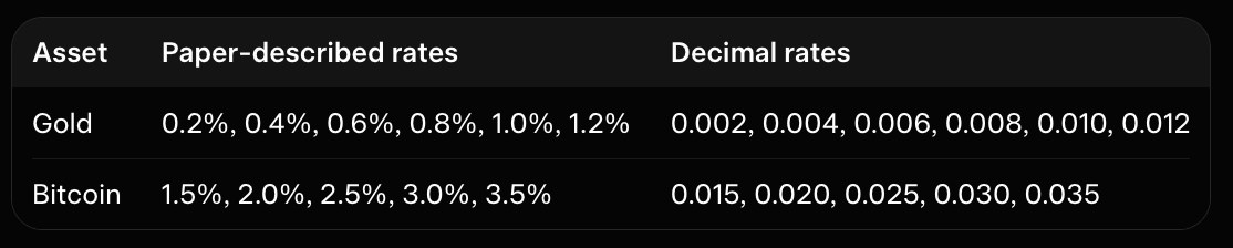
FeeSensitivityConfig defines these fields:

@dataclass
class FeeSensitivityConfig:
    gold_rates: tuple[float, ...] = (
        0.002, 0.004, 0.006, 0.008, 0.010, 0.012
    )
    bitcoin_rates: tuple[float, ...] = (
        0.015, 0.020, 0.025, 0.030, 0.035
    )
    apply_to_buys: bool = True
    apply_to_sells: bool = True
    hold_signals_fixed: bool = True

A decimal rate of 0.002 means 0.2%. Passing 0.2 would mean 20% and would be a different experiment.

There is an important current implementation limitation: run_fee_sensitivity looks for configuration attributes named gold_fees and bitcoin_fees, but FeeSensitivityConfig defines gold_rates and bitcoin_rates. As generated, custom configured grids are therefore not reliably consumed; the function can fall back to its module-level default grids. This naming mismatch must be repaired before claiming that arbitrary FeeSensitivityConfig values control the sweep.

16.5 Fixed signals versus regenerated policy decisions

Fee sensitivity can answer two different questions.

Fixed-signal sensitivity

Generate forecasts and orders once, then replay the same orders under each fee rate:

same data
same forecasts
same signals
same sizing schedule
fee rate changes
backtest reruns

This isolates the direct accounting effect of fees.

Fee-aware policy sensitivity

Regenerate candidate actions for each fee rate when fees affect:

• whether an order is affordable;

• whether its expected return exceeds its cost;

• which greedy candidate has the highest score; or

• whether exposure or risk constraints permit it.

The current run_fee_sensitivity function accepts a run_backtest callback and passes fee_rate to that callback:

def run_fee_sensitivity(
    run_backtest: Callable[..., Any],
    *,
    asset: str,
    config: FeeSensitivityConfig | None = None,
    fees: Sequence[float] | None = None,
    base_kwargs: Mapping[str, Any] | None = None,
) -> list[ExperimentResult]:

This callback-based design is intentional infrastructure, not direct strategy integration. The callback must decide whether to reuse signals or regenerate them. The current function does not inspect or enforce FeeSensitivityConfig.hold_signals_fixed, and it does not currently record an explicit signals_fixed or policy_regenerated field. Its hardcoded metadata field non_fee_assumptions_held_fixed=True only states the intended sweep contract; it does not establish how the callback selected actions.

A repaired orchestration contract should record the policy mode explicitly, for example:

result.metadata.update(
    {
        "fee_rate": rate,
        "fee_percent": rate * 100.0,
        "signals_fixed": True,
        "policy_regenerated": False,
        "non_fee_assumptions_held_fixed": True,
    }
)

For a fee-aware callback, the last two policy fields should instead indicate that decisions were regenerated. Until that metadata and configuration handling are aligned, fee-sweep results should be treated as callback outputs whose policy behavior must be inspected separately.

16.6 Optional benchmark orchestration

run_forecast_experiment(include_benchmarks=True) is intended to request the optional benchmark suite. However, the generated call currently passes names such as train_data and test_data, while run_benchmark_suite requires train_values and test_values. The compatibility helper filters keyword arguments but cannot invent missing required parameter names. Consequently, the benchmark path may fail and be converted into a warning rather than producing benchmark results.

The required interface should be aligned explicitly, for example:

benchmark = run_benchmark_suite(
    train_values=train_data,
    test_values=test_data,
    metadata={"asset": asset, "horizon": horizon},
)

Until that repair is made, benchmark orchestration should be described as an intended dispatch path, not as a verified working connection. Optional dependency status and model semantics remain important: HMM Viterbi decoding is not automatically a price forecast, and XGBoost is gradient-boosted trees rather than a random forest. Benchmark metrics also require aligned targets, timestamps, preprocessing, and untouched test data.

16.7 Recording results and paper claims

The result layer can save local artifacts:

def save_local_results(
    results: ExperimentResult | Iterable[ExperimentResult],
    path: str | Path,
    *,
    format: str | None = None,
) -> Path:

JSON preserves nested predictions, warnings, and metadata. CSV is convenient for scalar comparison tables. Neither format establishes empirical validity.

The paper's headline outcomes are stored as claims rather than expected outputs:

PAPER_REPORTED_VALUES = {
    "gold_final_value_usd": {
        "value": 646.0,
        "status": "reported_unverified_claim",
    },
    "bitcoin_final_value_usd": {
        "value": 215487.0,
        "status": "reported_unverified_claim",
    },
    "combined_final_value_usd": {
        "value": 216133.0,
        "status": "reported_unverified_claim",
    },
}

These values must not be used as unit-test expectations. The original data, dates, signals, sizing equations, VaR settings, greedy rules, fee convention, and liquidation protocol are missing. Agreement with one number would not prove that the full method was reproduced; disagreement under a different local protocol would not by itself identify a coding error.

16.8 What a trustworthy fee-sensitivity record should contain

Each scenario should preserve at least:

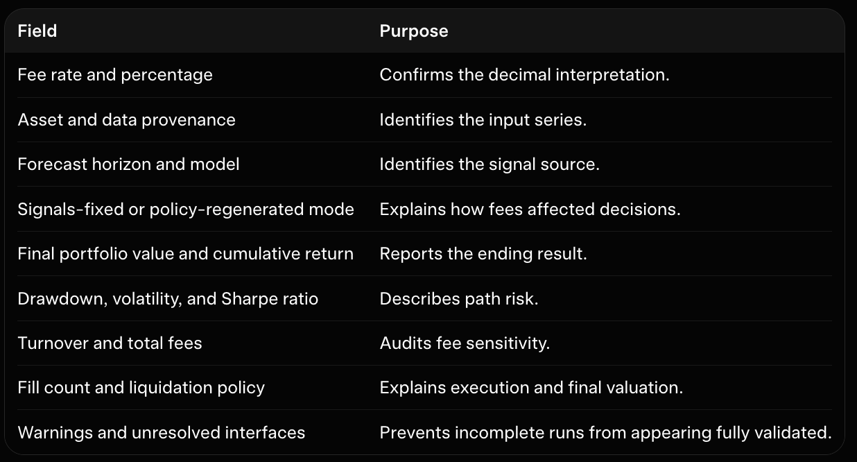
The current summarize_results function flattens scalar fields from result metrics, portfolio summaries, and metadata. save_local_results writes those records locally. Before relying on the files, inspect whether the callback supplied portfolio fields and whether policy metadata accurately describes the run.

16.9 Practical checklist and current readiness

Before preparing a forecast or fee experiment, record:

Local data path and provenance.

Asset, instrument, currency, frequency, and date range.

Window length, stride, target representation, and horizon.

Chronological or walk-forward boundaries.

Scaling method and fitting rows.

Model architecture, seed, and optional dependency versions.

Signal aggregation and thresholds.

Sizing schedule and exposure limits.

VaR confidence, horizon, lookback, and action mode.

Fee convention, slippage, execution timing, and liquidation policy.

Whether signals are fixed or regenerated for each fee scenario.

Forecast metrics and portfolio metrics in separate fields.

Any warnings caused by unavailable dependencies or API mismatches.

The generated project should currently be treated as a static, educational artifact rather than an executed experiment system. Known issues include the timestamp argument mismatch in standardize_prices, the benchmark argument-name mismatch, the unused hold_signals_fixed setting, and the fee-grid naming mismatch. Static checks also reported findings in experiments.py, while semantic code verification was skipped. Therefore, this section documents the intended orchestration contracts and the current limitations without claiming that the experiment paths were executed or that their outputs are correct.

16.10 Interpreting the missing fee figures

The fee grids can be reproduced as an experiment design. The paper's numerical curves cannot be recovered from the extracted text. Do not infer them from the headline profits, interpolate them from the listed percentages, or label a newly generated local curve as the paper's result.

A local result should instead be described as:

performance under the repository's documented reconstruction and local dataset

That wording preserves the value of sensitivity analysis while distinguishing it from empirical reproduction. The experiment layer's current contribution is reproducible configuration and result recording; direct end-to-end trading orchestration remains a repair task rather than an implemented fact.

17. Run the Offline Workflow from the Command Line

The project defines an offline command-line interface (CLI) for inspecting local data, generating synthetic demonstrations, and requesting research experiments. It does not connect to an exchange, download prices, store credentials, or submit orders.

The CLI should therefore be understood as a documented interface around the research modules, not as a verified end-to-end trading application. Several generated integrations currently have known incompatibilities. The examples below describe the intended command contracts and identify where the generated files still require repair. No command execution is claimed.

17.1 Command registration and optional dependencies

The shell command is registered in pyproject.toml:

[project.scripts]
quant-trading-model = "quantitative_trading_model.cli:main"

After installation, this maps quant-trading-model to main() in src/quantitative_trading_model/cli.py. The parser selects a subcommand and the handler produces local output.

Modeling dependencies are optional:

[project.optional-dependencies]
deep-learning = ["torch>=2.0"]
classical = [
    "statsmodels>=0.14",
    "pmdarima>=2.0",
    "hmmlearn>=0.3",
    "xgboost>=2.0"
]

The core data, streak, sizing, risk, and accounting modules use the lighter dependencies declared in the main project configuration. PyTorch and classical forecasting packages are imported only by features that need them.

The intended behavior is to report a missing optional dependency clearly. However, the generated main() catches CLIError, FileNotFoundError, ValueError, and TypeError, but not ImportError. Consequently, a missing PyTorch installation may still produce an uncaught traceback when a forecast command reaches the model layer. The CLI needs an explicit except ImportError branch before this behavior can be described as reliable shell-level error handling.

17.2 Defined subcommands

build_parser() defines these subcommands:

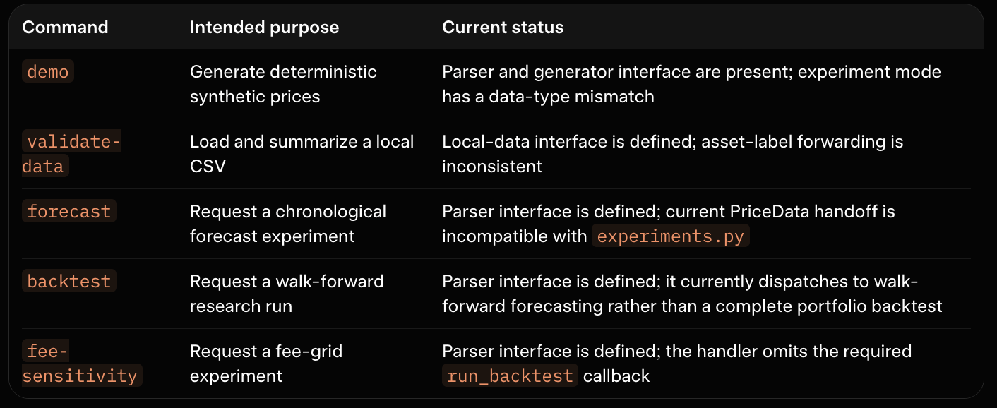
Thus, the commands are statically specified interfaces, not all working workflows. A complete runtime path requires repairing the interfaces identified below.

The parser excerpt illustrates the command structure:

def build_parser() -> argparse.ArgumentParser:
    parser = argparse.ArgumentParser(
        prog="quant-trading-model",
        description="Offline educational tools for the quantitative trading model paper.",
    )
    subparsers = parser.add_subparsers(dest="command", required=True)

    demo = subparsers.add_parser("demo")
    demo.add_argument("--rows", type=int, default=500)
    demo.add_argument("--seed", type=int, default=7)
    demo.add_argument("--asset", choices=("gold", "bitcoin"), default="gold")
    demo.set_defaults(handler=run_demo)

    # validate-data, forecast, backtest, and fee-sensitivity are
    # registered later in the same function.
    return parser

This is an explanatory excerpt, not a complete replacement for cli.py.

17.3 Local-only paths and data provenance

The CLI includes path checks intended to reject URLs and network paths:

def _safe_input_path(value: str) -> Path:
    if "://" in value:
        raise CLIError("Only local files are supported; URLs and network paths are not accepted")
    path = Path(value).expanduser()
    if not path.exists():
        raise CLIError(f"Input file does not exist: {path}")
    if not path.is_file():
        raise CLIError(f"Input path is not a regular file: {path}")
    return path.resolve()


def _safe_output_path(value: str) -> Path:
    if "://" in value:
        raise CLIError("Output must be a local path, not a URL")
    path = Path(value).expanduser()
    if path.exists() and path.is_dir():
        raise CLIError(f"Output path is a directory: {path}")
    return path.resolve()

These checks constrain file locations; they do not establish that a dataset matches the paper. Every local result should also record the source file, instrument, currency, frequency, date range, timezone, cleaning rules, and configuration snapshot.

There is a further generated-file inconsistency in _load_local_data(): it passes asset_name=args.asset, while the generated load_price_csv() function accepts asset, not asset_name. Depending on the compatibility wrapper, this can fail or cause the loader to retain its default asset label. The keyword must be aligned before asset-specific provenance can be trusted.

17.4 Synthetic demonstration

The intended synthetic command is:

quant-trading-model demo \
  --rows 500 \
  --asset gold \
  --seed 7 \
  --output results/demo.json

run_demo() calls generate_synthetic_prices() and records a compact summary. Synthetic data are useful for teaching timestamp handling, window construction, tensor shapes, finite sizing, VaR decisions, and portfolio accounting. They are not historical gold or Bitcoin data and cannot reproduce the paper's reported outcomes.

The optional --run-experiment flag is currently not a complete path. The generator returns a PriceData object, and run_demo() passes that object to run_forecast_experiment(). In the generated experiments.py, _price_array() handles a pandas Series, a pandas DataFrame, or an array-like object, but does not handle PriceData. The experiment can therefore fail before window construction. The repair must either teach _price_array() to extract PriceData.frame or make the CLI pass a compatible DataFrame or Series.

This same PriceData mismatch affects the forecast handler, because _load_local_data() also returns PriceData and passes it to run_forecast_experiment(). These commands are therefore documented as intended interfaces until that data contract is repaired.

17.5 Validate a local CSV

The generated parser uses a positional CSV argument. A statically accurate example is:

quant-trading-model validate-data data/gold.csv \
  --timestamp-column timestamp \
  --price-column close \
  --asset gold \
  --output results/gold_data_summary.json

run_validate_data() is intended to:

check the local path;

call load_price_csv();

summarize the resulting object; and

print or write local JSON.

The loader requires parseable timestamps and finite, positive prices, and it sorts and deduplicates observations. The summary should be saved with a provenance record rather than treated as evidence that the data are the same data used by the paper.

Some older README examples use --input data/gold.csv, but the generated parser defines csv positionally and does not define an --input option. The positional form above matches the generated CLI more closely.

17.6 Forecast command: intended interface and current limitation

The intended command is:

quant-trading-model forecast data/gold.csv \
  --timestamp-column timestamp \
  --price-column close \
  --asset gold \
  --output results/gold_forecast.json

Optional benchmarks are requested with:

quant-trading-model forecast data/gold.csv \
  --timestamp-column timestamp \
  --price-column close \
  --asset gold \
  --benchmarks \
  --output results/gold_forecast_with_benchmarks.json

The intended data flow is:

local CSV
  -> local loader
  -> standardized prices
  -> 100-observation windows
  -> chronological split
  -> Att-BiLSTM or selected forecaster
  -> forecast metrics
  -> local result artifact

The current generated path is not yet a verified runtime workflow. The CLI passes PriceData into run_forecast_experiment(), while _price_array() in experiments.py does not extract PriceData. This must be repaired before the command can reliably reach the forecasting model.

Even after that data mismatch is fixed, a missing PyTorch installation may escape through main() as an uncaught ImportError. The CLI should catch that exception and convert it into an actionable message. Until then, the optional-dependency behavior is a model-layer intention, not a guaranteed CLI behavior.

A repaired forecast artifact should include the asset, model, window length, horizon, split protocol, seed, preprocessing decisions, forecast metrics, package versions, and warnings. Forecast metrics remain separate from portfolio metrics and do not measure fees, turnover, drawdown, or liquidation.

17.7 Backtest command: distinguish forecasting from portfolio simulation

The intended command is:

quant-trading-model backtest data/bitcoin.csv \
  --timestamp-column timestamp \
  --price-column close \
  --asset bitcoin \
  --output results/bitcoin_backtest.json

In the generated CLI, run_backtest_command() calls run_walk_forward_experiment(). That function is intended to evaluate sequential forecasts; it does not, by itself, compose forecast signals, exponential sizing, VaR, greedy action selection, fills, fees, and portfolio valuation.

The repository does contain separate strategy and accounting modules. A complete portfolio backtest must explicitly connect them:

walk-forward forecast
  -> signal generation
  -> finite sizing
  -> VaR filter
  -> greedy action selection
  -> next-bar order
  -> portfolio simulator

Therefore, the current backtest command is a statically described walk-forward entry point, not proof that a complete paper trading strategy is running. Its name should not be interpreted as evidence that the paper's missing execution protocol has been recovered.

17.8 Fee-sensitivity command: parser exists, callback wiring is incomplete

The paper-inspired fee grids are:

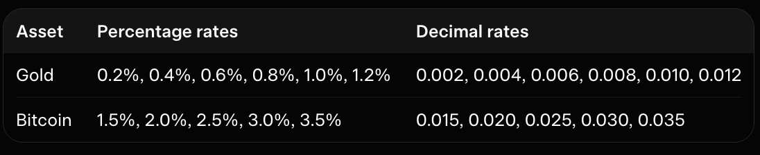
The intended command is:

quant-trading-model fee-sensitivity data/gold.csv \
  --timestamp-column timestamp \
  --price-column close \
  --asset gold \
  --output results/gold_fee_sensitivity.json

The command is currently only a parser-level interface. run_fee_sensitivity() in experiments.py requires a positional run_backtest callback, followed by the asset and fee configuration. However, run_fee_sensitivity_command() calls it without supplying that required callback. As written, the handler cannot successfully invoke the fee experiment.

A repair must construct or inject a callback that accepts fee_rate, runs the same strategy and data under that fee, and returns portfolio results. Only then can the CLI perform a sensitivity sweep. The callback should hold all non-fee assumptions fixed: data, dates, forecasts, signal rules, sizing, slippage, initial cash, and liquidation. If fees change feasibility or greedy ranking, decisions must be regenerated and that dependency recorded.

The missing numeric values in the paper's fee figures must not be inferred from the fee grid itself.

17.9 Optional dependency installation

The intended installation commands are:

python -m pip install -e .
python -m pip install -e '.[deep-learning]'
python -m pip install -e '.[classical]'

The generated pyproject.toml defines the classical extra. Some README text refers to a benchmarks extra, which is inconsistent; classical is the authoritative generated metadata name.

A missing optional package should ideally produce a message such as:

PyTorch is required for recurrent forecasters. Install the optional deep-learning dependencies for this project.

At present, the model layer can raise that message, but the CLI's main() does not catch ImportError. Repairing the exception handling is necessary for the message to be consistently presented as a normal command-line error.

17.10 Archive results with provenance

The CLI's output helper is intended to print JSON or write it to a local file:

def _write_output(value: Any, output: str | None) -> None:
    rendered = _dump(value)
    if output is None:
        print(rendered)
        return
    path = _safe_output_path(output)
    path.parent.mkdir(parents=True, exist_ok=True)
    path.write_text(rendered + "\n", encoding="utf-8")
    print(f"Wrote {path}")

A useful research directory might contain:

results/
├── gold_data_summary.json
├── gold_forecast.json
├── gold_fee_sensitivity.json
├── config_snapshot.json
├── package_versions.txt
└── provenance.md

The configuration snapshot should include the window length, target horizon, scaler policy, model settings, fee rate, slippage, VaR settings, sizing schedule, signal thresholds, execution timing, and liquidation policy. The provenance file should identify the local data file and instrument metadata.

The paper's approximate $646 gold value and $215,487 Bitcoin value remain unverified claims. A local JSON file without dates, data provenance, and execution assumptions cannot validate either number.

17.11 Offline workflow checklist

The intended research workflow is:

Install only the dependencies required for the selected module.

Inspect quant-trading-model --help and the relevant subcommand help.

Use demo to inspect synthetic data flow, without treating it as empirical evidence.

Use validate-data on each local asset file.

Save the data summary and provenance metadata.

Run a chronological forecast experiment after repairing the PriceData handoff.

Record model status, target horizon, metrics, seed, and configuration.

Run walk-forward evaluation for trading-oriented conclusions.

Connect forecasts explicitly to signals, sizing, VaR, greedy selection, and next-bar execution for a portfolio backtest.

Supply a valid backtest callback before using fee sensitivity.

Compare portfolio results with buy-and-hold and report drawdown, volatility, turnover, and fees.

Label every result as implemented, reconstructed, illustrative, unavailable, or reported claim as appropriate.

The generated CLI and orchestration files also have known static-review findings: placeholder detection was reported for cli.py, and semantic code verification was skipped. Some generated tests and orchestration calls are API-inconsistent with the generated modules. These findings reinforce the correct interpretation of this section: it documents intended offline interfaces and their current repair requirements; it does not claim that any command ran successfully.

The central lesson is that a CLI can make a research workflow repeatable in form, but it cannot supply missing data or algorithmic details. Reliable interpretation still requires local data provenance, explicit configuration, causal signal timing, repaired module interfaces, and a strict distinction between computed results and the paper's unverified claims.

18. Verification: Static, Semantic, and Invariant Checks

A paper-to-code project needs more than a collection of source files. It also needs a disciplined way to check whether the implementation is structurally coherent, whether its assumptions are visible, and whether its financial logic avoids obvious look-ahead errors. At the same time, verification must not be overstated. A file that parses successfully is not necessarily semantically correct, and a passing unit test would not prove that the paper's reported profits are reproducible.

For this project, verification has three layers:

Static verification checks source structure without running the research pipeline.

Semantic review checks whether the implementation matches the intended mathematics and data flow.

Empirical validation would compare executed results with the paper, but it is currently unavailable because the original data and protocol are missing.

The supplied local verification performed the first layer and recorded a partial result. Semantic code verification was explicitly skipped. Therefore, the discussion below describes the intended checks and the reported findings; it does not claim that the generated code was executed or that the test suite passed.

18.1 Static verification: checking structure without execution

Static checks inspect files as text or syntax trees. They are useful because they can identify malformed Python, missing symbols, accidental placeholders, unsafe patterns, and documentation inconsistencies before a runtime experiment is attempted.

The local verification report applied checks such as:

• non-empty file validation;

• detection of Markdown fences in generated code fields;

• placeholder and TODO detection;

• checks for live-trading patterns;

• generic text checks;

• Python AST parsing for Python files.

AST parsing is stronger than looking for balanced parentheses with a text search. It asks Python's parser whether a file has valid syntax and produces a structured representation of imports, classes, functions, and statements. It does not, however, prove that imported names exist at runtime or that two modules agree on an API.

The static checks reported successful parsing and structural checks for the core modules, including:

• data.py, which constructs windows and chronological partitions;

• metrics.py, which separates forecast and portfolio measures;

• models/attention.py and models/forecasters.py, which define the tensor-facing model interfaces;

• streaks.py, sizing.py, and risk.py, which implement the reconstructed analytical components;

• strategy.py and backtest.py, which define candidate actions and portfolio accounting; and

• the generated test files.

That result gives useful confidence that these files are non-empty and syntactically parseable. It does not establish that the modules can be imported together, that optional dependencies are available, or that the implementation behaves correctly for real data.

18.2 Reported static-check findings

The overall local static-verification result was not passing. Four generated files were reported with issues:

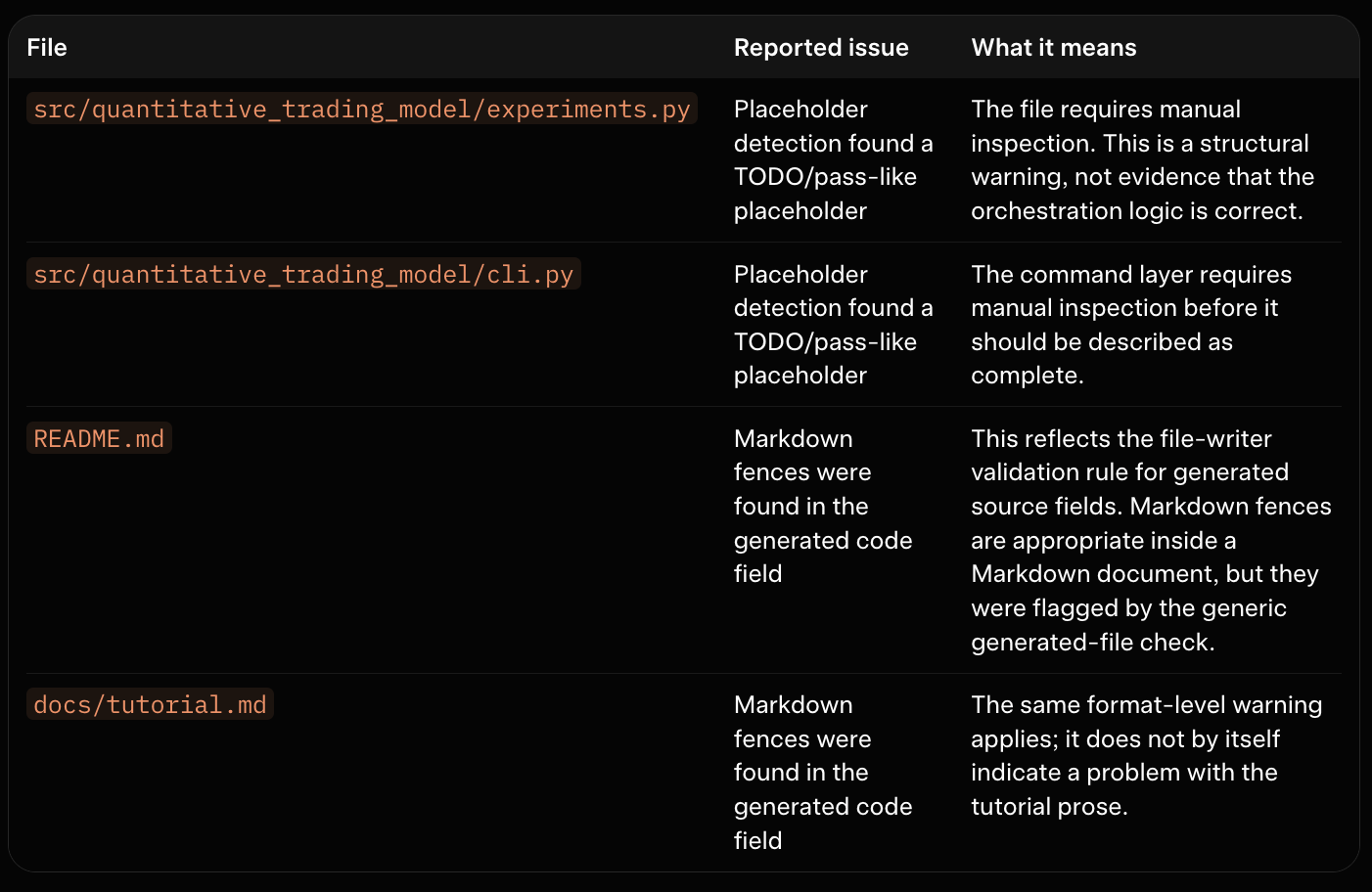
The Markdown findings are format warnings in the generated-file representation. A Markdown tutorial normally uses fenced code blocks, so removing every fence would make the document less useful to readers. The important distinction is between a validation rule for a generated code field and the normal syntax of a Markdown document.

The placeholder findings are more substantive. They should be reviewed manually because a placeholder can mean anything from an intentionally unfinished branch to an incomplete implementation. Until that review and repair occur, the experiment and CLI layers should be described as planned or partially integrated artifacts rather than as verified end-to-end interfaces.

18.3 Semantic review: checking meaning, not just syntax

Semantic verification asks whether the code's operations match the intended method. For this project, the most important semantic questions are temporal, mathematical, and accounting-related.

Temporal and data invariants

The windowing and data tests are intended to review the following properties:

• timestamps are strictly increasing after cleaning;

• prices are finite and positive;

• a target timestamp occurs after the final timestamp in its input window;

• chronological training and test partitions remain ordered;

• scaling parameters are fitted only on training observations; and

• no forecast uses a target or realized return from the future.

These checks matter because a time-series implementation can be syntactically valid while still leaking information. For example, fitting a scaler on the complete series or randomly mixing overlapping windows can make a forecast evaluation look stronger than a deployment-like evaluation.

The test file tests/test_data_and_streaks.py is designed around small hand-calculated paths. That is a good verification strategy for boundaries: a short sequence makes it possible to calculate the expected target values and return signs manually. It is more informative for temporal invariants than a large opaque fixture.

Attention and model-shape invariants

The model tests are intended to review tensor contracts rather than predictive quality. The key conditions are:

• recurrent inputs have shape (batch, time, features);

• attention scores have shape (batch, time);

• attention weights are nonnegative;

• weights sum to one across the time dimension;

• the context vector has shape (batch, features);

• one-step and three-step heads return the configured horizon; and

• the primary model contains the configured 20% dropout layer.

The attention normalization check is particularly important. Applying softmax across features instead of time would produce a different algorithm from the paper's temporal attention equations. Shape tests can catch that kind of error without claiming that the model has learned a useful forecast.

The model tests also need PyTorch-aware handling. PyTorch is optional in this project, so a minimal installation should skip tensor-execution tests cleanly rather than fail while importing unrelated data or accounting modules. A skipped optional test is not a passing model validation; it means that the environment did not perform that check.

Streak and return invariants

The streak tests review the reconstruction of the paper's consecutive-rise and decline analysis:

• the default simple return uses the previous price as denominator;

• zero returns do not silently become rises or declines;

• maximal runs and overlapping subsequences produce different, intentional counts;

• streak counts are nonnegative integers; and

• percentile calculations use only the supplied historical segment.

These checks are important because the paper's use of the term “Apriori” is not operationally supported by frequent-itemset support or confidence calculations. The implementation should therefore be reviewed as streak analysis, with its chosen return and zero policies recorded explicitly.

Position-sizing invariants

The sizing tests should confirm that the normalized exponential reconstruction remains bounded:

• every score and allocation is finite and nonnegative;

• normalized weights sum to one within tolerance;

• the planned allocations do not exceed the schedule budget;

• an addition level cannot be consumed twice accidentally;

• the approved amount cannot exceed available cash; and

• the exposure cap prevents unlimited averaging down.

These are safety and consistency properties of the reconstruction. They do not prove that the paper's corrupted equations (5)–(8) were recovered correctly. In fact, exact verification of those equations remains unavailable until the original notation or equation images are supplied.

VaR and strategy invariants

The risk and strategy layers require a different kind of semantic review. The intended checks include:

• VaR uses only returns available before the decision timestamp;

• insufficient history is represented explicitly;

• a blocked trade receives zero approved quantity;

• risk scaling never increases the proposed order;

• candidate scores use forecasts, current portfolio state, fees, and constraints only;

• infeasible actions are excluded before ranking; and

• greedy tie-breaking is deterministic.

These conditions prevent a risk filter from becoming decorative. A VaR calculation that uses future returns, or a strategy score that accidentally includes realized profit, would invalidate the backtest even if every function returns a number.

The paper does not define its VaR parameters or greedy objective. Consequently, semantic verification can check the internal consistency of the chosen reconstruction, but it cannot check fidelity to an unavailable original algorithm.

Portfolio-accounting invariants

The backtest tests are designed around hand-computable transactions. The central identity is:

\[ Vt = \operatorname{cash}t + \operatorname{quantity}t pt. \]

The intended accounting checks include:

• every fill occurs after its signal timestamp;

• buy and sell fees are applied exactly once to executed notional;

• unaffordable buys do not create negative cash under no-leverage settings;

• holdings do not become negative when shorting is disabled;

• marked portfolio value equals cash plus marked holdings;

• liquidation is explicit; and

• the buy-and-hold benchmark follows a documented fee and timing convention.

These tests verify the simulator's stated accounting contract. They do not verify the paper's accounting because the paper does not specify its execution dates, fee-side convention, slippage, partial-unit rules, or liquidation policy.

18.4 Why the skipped semantic verification matters

The semantic verification report states that code semantic verification was skipped using the --skip-code-semantic-verification option. Its overall assessment was therefore “not semantically reviewed.” This is an important limitation, not a minor footnote.

Static AST parsing can show that Python syntax is valid. It cannot reliably detect every issue that a semantic review would investigate, such as:

• a caller passing split_config to a function that accepts only config;

• a test constructing a class with fields that differ from the generated class;

• a benchmark adapter assuming a metric method that another module does not expose;

• a forecast output using a different shape from the target array; or

• an experiment function describing end-to-end backtesting while only orchestrating forecasts.

The supplied project notes also warn that some generated tests and orchestration code appear API-inconsistent with the generated modules. That means the tests should be treated as intended invariant specifications and static artifacts until their interfaces are reconciled. No claim should be made that the test suite passes.

18.5 Verification is not execution and execution is not reproduction

There are three separate statements that should not be conflated:

The source parses. Python's parser accepted the file structure.

The implementation is semantically coherent. Functions, types, formulas, and timestamps agree with one another under review.

The paper's experiment is reproduced. The implementation matches the original data, protocol, and reported results.

The available evidence supports only parts of the first statement. The second was not completed by the supplied semantic verifier. The third is impossible at present because the paper's data and several algorithmic details are missing.

In particular, this tutorial does not claim that:

• the generated code was executed;

• all dependencies were installed;

• the tests passed;

• the CLI completed a forecast or backtest;

• the reported $646 gold value or $215,487 Bitcoin value was reproduced; or

• the paper's benchmark metrics or fee-sensitivity curves were confirmed.

The correct interpretation is narrower: the project contains intended implementations, tests, and verification rules, while the local static report identifies both successful structural checks and unresolved findings.

18.6 A practical review order

When repairing or extending the project, review the layers in this order:

Resolve format and placeholder findings. Inspect experiments.py and cli.py; decide whether each detected placeholder is intentional or incomplete. Treat the Markdown-fence findings as representation warnings where fences are normal Markdown syntax.

Reconcile public APIs. Compare function signatures and dataclass fields across source modules and tests. In particular, check the experiment-to-data, strategy-to-risk, and test-to-sizer interfaces.

Run syntax and import checks in the target environment. Confirm that core imports do not require optional PyTorch or benchmark packages, and that optional failures are explicit.

Review data boundaries. Hand-check window endpoints, target timestamps, scaler fitting, and chronological splits.

Review tensor shapes. Confirm attention normalization across time and forecast-target horizon agreement.

Review pure analytical components. Check return denominators, streak policies, normalized sizing, and VaR sign conventions with small numerical examples.

Review portfolio accounting. Reconcile every fill, fee, cash change, holding quantity, and mark-to-market value.

Only then run local experiments. Preserve configuration, data provenance, software versions, warnings, and result metadata.

Compare with the paper cautiously. Label any mismatch as unresolved unless the original data and protocol are available.

This order moves from inexpensive structural checks to more demanding semantic and empirical work. It also prevents a striking backtest number from distracting attention from basic timestamp or accounting errors.

18.7 Reproduction status remains a separate question

The reproduction matrix in docs/reproduction_matrix.md is the appropriate place to track paper fidelity. It distinguishes direct mechanics—such as temporal attention equations, window construction, and portfolio identities—from reconstructions such as normalized exponential sizing, historical VaR, and greedy action selection.

A useful final status summary is:

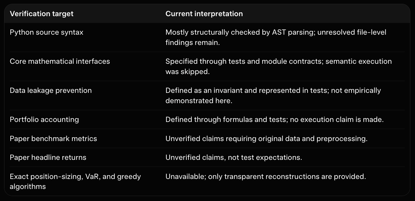
The purpose of this verification process is therefore not to manufacture certainty. It is to make uncertainty inspectable: readers can see which files parse, which invariants are intended, which findings remain unresolved, and which paper claims cannot yet be tested. That is the appropriate standard for an educational implementation of an incompletely specified quantitative-trading paper.

19. Worked Synthetic Example from Price Path to Portfolio Record

This section connects the data, streak, sizing, risk, strategy, and accounting layers with a short synthetic price path:

prices: 100, 102, 101, 99, 100, 103

The example follows this causal sequence:

prices
  → standard returns and streaks
  → manually supplied forecast
  → finite position-size schedule
  → VaR decision
  → greedy candidate selection
  → next-bar fill
  → portfolio valuation

This is an illustrative interface example, not an empirical backtest. The prices are synthetic and the forecast is supplied manually rather than produced by a trained model. The paper's exact position-sizing equations, VaR procedure, and greedy policy are unavailable, so those components remain documented reconstructions. The code was not executed here; the calculations below describe the intended contracts and hand-checkable accounting.

19.1 Prepare the synthetic prices

The data layer accepts local historical data. For a small example, create a pandas Series and convert it into the standard timestamp-and-price table:

import pandas as pd

prices = pd.Series(
    [100.0, 102.0, 101.0, 99.0, 100.0, 103.0],
    index=pd.date_range("2024-01-01", periods=6, freq="D"),
    name="price",
)

from quantitative_trading_model.data import standardize_prices

clean = standardize_prices(
    prices.rename_axis("timestamp").reset_index(),
    timestamp_column="timestamp",
    price_column="price",
    asset="synthetic",
)

standardize_prices parses timestamps, sorts observations, removes invalid rows when configured to do so, resolves duplicate timestamps, and returns a PriceData object. Prices must be finite and strictly positive. The function does not identify a market-data source or make network requests.

Six observations are far shorter than the paper-inspired 100-observation forecasting window. This path is therefore unsuitable for training the Att-BiLSTM. It is only long enough to demonstrate return alignment, decision timing, and portfolio accounting.

19.2 Compute standard returns

The default reconstruction uses the conventional simple return:

\[ rt = \frac{pt-p{t-1}}{p{t-1}}. \]

from quantitative_trading_model.streaks import compute_returns

returns = compute_returns(clean.prices, denominator="previous")

The hand calculations are:

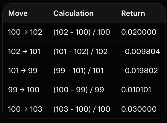
Each return is aligned to the later price. Thus, the return from 101 to 99 becomes known at the 99-price observation. It must not be assigned to the earlier 101 timestamp when constructing an online risk history.

The extracted paper equation appears to use the current price as the denominator. That alternative is available through denominator="current" or denominator="paper", but one convention must be used consistently throughout a given experiment.

19.3 Classify movements and identify streaks

The sign sequence is:

+  -  -  +  +

The streak layer separates calculation, classification, and counting:

from quantitative_trading_model.streaks import classify_returns, count_streaks

labels = classify_returns(returns, zero_policy="neutral")

rise_counts = count_streaks(
    labels,
    value=1,
    mode="maximal",
    minimum_length=1,
)
decline_counts = count_streaks(
    labels,
    value=-1,
    mode="maximal",
    minimum_length=1,
)

The maximal runs are:

positive run of length 1
negative run of length 2
positive run of length 2

Conceptually, the results are:

rise_streaks:    {1: 1, 2: 1}
decline_streaks: {2: 1}

count_streaks also supports mode="overlapping". A run of four positive returns contains three overlapping two-return subsequences, whereas maximal mode records one complete run of length four. These statistics are different, and the paper does not specify which one it used.

A complete summary can be requested with:

from quantitative_trading_model.streaks import compute_streak_statistics

stats = compute_streak_statistics(
    clean.prices,
    denominator="previous",
    zero_policy="neutral",
    streak_mode="maximal",
)

print(stats.gain_percentile_90)
print(stats.decline_percentile_10)
print(stats.rise_streaks)
print(stats.decline_streaks)

The summary exposes the 90th-percentile gain, signed 10th-percentile decline, median gain, and decline magnitudes. With only five returns, these estimates are not statistically meaningful. In a real walk-forward experiment, the statistics must be calculated from observations available before the relevant decision.

This implementation calls the procedure streak analysis or sequential-pattern analysis, not standard Apriori. The paper does not provide Apriori itemsets, support, or confidence calculations.

19.4 Build and consume a finite sizing level

The paper's equations (5)–(8) are incomplete in the extracted source. The implementation therefore uses a normalized exponential reconstruction. Suppose the schedule has a $300 budget and three addition levels:

from quantitative_trading_model.sizing import (
    ExponentialPositionSizer,
    build_exponential_schedule,
)

schedule = build_exponential_schedule(
    budget=300.0,
    max_additions=3,
    growth=0.50,
    amplitude=1.0,
)
sizer = ExponentialPositionSizer(schedule=schedule)

print(schedule.weights)
print(schedule.allocations)

The reconstructed scores have the form:

si=Aexp⁡(Bi),

followed by normalization:

\[ wi=\frac{si}{\sumj sj}, \qquad \operatorname{allocation}i=300wi. \]

For indices i = 0, 1, 2, A = 1, and B = 0.5, the scores are approximately:

1.0000, 1.6487, 2.7183

The resulting planned allocations are approximately:

level 1: $55.89
level 2: $92.16
level 3: $151.95

The first schedule level is not merely described as selected: it is connected to the strategy through ExponentialPositionSizer. The strategy uses one-based addition levels in its public action record, while the schedule stores zero-based Python indices internally. After the action is approved, the selected level is consumed exactly once:

allocation = sizer.allocate_next_addition(
    available_cash=500.0,
    current_exposure=0.0,
)

print(allocation.level)          # first internal level is 0
print(allocation.approved_amount)

The allocation cannot exceed available cash or the configured exposure capacity. This is a finite schedule, not unlimited averaging down. The formula and any calibration from gains, declines, or fees are reconstructions rather than faithful transcriptions of the paper's unreadable recursive break-even equations.

19.5 Produce a forecast-derived signal

Assume that when the observed price is 99, a forecasting model predicts a one-step price of 101. The forecast is manually supplied for this example:

rforecast=10199−1≈0.020202.

That is an expected increase of about 2.02%.

from quantitative_trading_model.strategy import SignalGenerator

signal_generator = SignalGenerator(
    buy_threshold=0.01,
    sell_threshold=0.01,
    aggregation="terminal",
)

decision = signal_generator.decide(
    current_price=99.0,
    forecasts=[101.0],
)

print(decision.signal)
print(decision.expected_return)

The expected increase exceeds the 1% buy threshold, so the intended signal is Signal.BUY. SignalGenerator.decide uses only the current price and forecast. It does not receive the later realized prices of 100 or 103.

For a three-day forecast, the same class can aggregate values such as [100.0, 101.0, 102.0]. The default terminal policy uses the final forecast; mean and max are also available. The paper mentions three-day forecasts but does not define this aggregation rule, so it remains an explicit reconstruction choice.

19.6 Apply historical VaR before ranking actions

The paper names VaR but does not specify its confidence level, horizon, lookback, or action rule. This example uses a rolling historical estimator with enough pre-decision observations to produce an estimate:

from quantitative_trading_model.config import VaRConfig
from quantitative_trading_model.risk import HistoricalVaR, VaRTradeFilter

var_config = VaRConfig(
    enabled=True,
    confidence=0.95,
    horizon=1,
    lookback=100,
    min_observations=3,
    action="scale",
    insufficient_history="allow",
    max_var_fraction=0.05,
)

var_estimator = HistoricalVaR(var_config)
var_filter = VaRTradeFilter(config=var_config)

At the 99-price decision point, the returns known from the path are the first three values:

pre_decision_returns = returns[:3]
estimate = var_estimator.estimate(pre_decision_returns)
print(estimate.var)
print(estimate.return_quantile)

The estimator now has three observations, matching the configured minimum. This is still only a toy quantile estimate; it is not a meaningful risk model. If the lower-tail return quantile were -1.8%, an exposure of $55.89 would imply an estimated loss of roughly:

55.89×0.018≈$1.01.

The actual estimate should be read from estimate, not inferred from this hypothetical number.

The risk decision uses currency notional units:

risk_decision = var_filter.decide(
    proposed_quantity=55.89,
    current_exposure=0.0,
    portfolio_value=500.0,
    returns=pre_decision_returns,
)

print(risk_decision.action)
print(risk_decision.approved_quantity)
print(risk_decision.reason)

Here, proposed_quantity is the VaR module's name for a proposed currency notional. It is not asset quantity. A positive approved amount means the risk filter accepted or scaled the proposed notional; a blocked trade has an approved amount of zero. The filter uses only the supplied pre-decision returns.

19.7 Rank the forecast and sizing candidates

The sizing schedule and risk decision are now connected explicitly. The risk-approved amount is passed as the maximum buy notional, while the sizer supplies the next addition level:

from quantitative_trading_model.strategy import GreedyPolicy, PortfolioSnapshot

approved_notional = float(risk_decision.approved_quantity)

snapshot = PortfolioSnapshot(
    cash=500.0,
    holdings=0.0,
    price=99.0,
    addition_level=0,
    portfolio_value=500.0,
)

policy = GreedyPolicy(fee_rate=0.002)
selected = policy.choose(
    snapshot,
    forecasts=[101.0],
    signal_generator=signal_generator,
    sizer=sizer,
    max_additions=3,
    buy_notional=approved_notional,
    returns=pre_decision_returns,
)

print(selected.signal)
print(selected.notional)
print(selected.addition_level)

This call does not pass VaRTradeFilter into GreedyPolicy. The VaR decision has already been applied directly with the compatible VaRTradeFilter.decide interface. That explicit separation avoids confusing a currency-notional risk result with an asset-unit order.

The candidate set conceptually contains:

hold:  score 0
buy:   risk-approved notional, using current cash
add:   next unused finite sizing level
sell:  unavailable because holdings are zero

The reconstructed greedy score for a buy or add action is:

score(a)=N(rforecast−f),

where N is currency notional, r_forecast is the predicted return, and f is the fee rate. If N = 55.89, r_forecast ≈ 0.020202, and f = 0.002, then:

score≈55.89(0.020202−0.002)≈1.02.

The hold candidate has score zero, so a positive approved buy or add candidate can outrank it. The actual selected amount must still be read from selected.notional; the paper does not define its own greedy objective or candidate set.

The GreedyPolicy call uses forecast information, current portfolio state, fees, and the already-approved risk amount. It does not use the later realized 99-to-100 return. That restriction prevents look-ahead bias.

19.8 Consume the selected schedule level

The strategy's selected addition level is an action description. The sizing schedule should consume its corresponding level only after the action has been accepted for execution:

if selected.signal.value == "add" and selected.addition_level is not None:
    allocation = sizer.allocate_next_addition(
        available_cash=snapshot.cash,
        current_exposure=snapshot.holdings * snapshot.price,
        level=selected.addition_level - 1,
    )
    print(allocation.approved_amount)

The subtraction converts the strategy's one-based public level to the sizer's zero-based schedule index. In a production orchestration layer, the approved amount returned by the sizer and the amount sent to the order should be compared explicitly. If risk scaling or cash caps reduce the amount, the order must use the reduced approved notional rather than the original planned allocation.

19.9 Execute on the next bar and calculate portfolio value

The signal is formed at the 99-price observation. The next bar has price 100, so the order executes at 100 rather than at the signal price of 99.

The example uses these units:

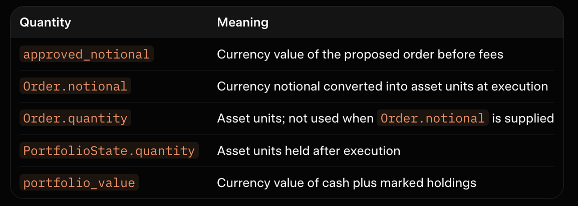
Assume the approved notional is $55.89, execution price is $100, the fee is 0.002, and slippage is zero. The hand calculation is:

q=55.89100=0.5589 units,

fee=55.89×0.002=$0.11178,

cash after buy=500−55.89−0.11178=$443.99822.

Immediately after the fill, the marked portfolio value is:

V=443.99822+0.5589×100=$499.88822.

The difference from $500 is the purchase fee.

The corresponding accounting objects are:

from quantitative_trading_model.backtest import Order, PortfolioSimulator

simulator = PortfolioSimulator(
    initial_cash=500.0,
    fee_rate=0.002,
    slippage_rate=0.0,
    allow_short=False,
    allow_leverage=False,
)

order = Order(
    side="buy",
    notional=55.89,
    signal_timestamp="2024-01-04",   # the bar priced at 99
    execution_timestamp="2024-01-05",
    addition_level=1,
    reason="forecast recovery signal",
)

fill = simulator.execute(order, "2024-01-05", 100.0)
record = simulator.mark_to_market("2024-01-05", 100.0)

print(fill.notional, fill.fee)
print(record.portfolio_value)

Order.notional is deliberately used here because the strategy and VaR layers work in currency-notional terms. The simulator converts that notional into asset units at the execution price. If an order instead supplies Order.quantity, the simulator treats it as asset units directly.

PortfolioSimulator.execute applies configured slippage, calculates executed notional and fees, updates cash and holdings, and records a Fill. mark_to_market creates a BacktestRecord satisfying:

\[ Vt=\text{cash}t+\text{quantity}t pt. \]

The default simulator is long-only and non-leveraged. It clips an unaffordable buy to the quantity affordable with current cash; the current generated execution path does not implement a separate rejection branch for the reject_insufficient_cash configuration field. That behavior should therefore not be described as configurable rejection without a corresponding backtest-code change.

If the price later reaches 103, the marked value before selling is approximately:

443.99822+0.5589×103≈$501.675.

A later sale would incur a second fee under the default two-sided fee convention. The final realized value would depend on the sale price, slippage, and whether end-of-test liquidation is enabled.

19.10 What the example demonstrates

The example makes the following contracts visible:

• returns are aligned with the later price observation;

• streaks are calculated from the selected return convention;

• the sizing schedule is finite, normalized, and connected to the action level;

• VaR is applied before the action is ranked;

• risk and strategy values are currency notionals, while backtest quantities are asset units;

• the greedy score uses forecasts and estimated fees, not realized future returns;

• the signal at price 99 executes at the later price of 100;

• the purchase fee is deducted exactly once;

• portfolio value equals cash plus marked holdings.

It does not demonstrate profitability. The forecast is manual, the price path is synthetic, and the paper's exact sizing, VaR, and greedy methods are unavailable. The example is a causal and accounting demonstration, not a reproduction of the paper.

19.11 Relation to the paper's reported outcomes

The paper reports approximately $646 from a $500 gold allocation and approximately $215,487 from a $500 Bitcoin allocation. Neither result can be inferred from this six-price example. Reproducing either claim would require the original datasets, dates, target definition, complete position-sizing equations, VaR settings, greedy rules, fee treatment, execution timing, and liquidation policy.

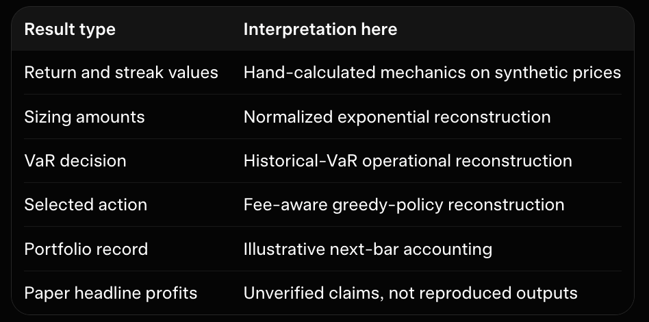
The example is useful because it makes causality, units, and accounting explicit. It should not be used as evidence about expected returns, investment quality, or the validity of the paper's headline performance.

20. Limitations, Interpretation, and What a True Reproduction Would Need

The implementation now expresses the paper’s main ideas as separate, inspectable components: an attention-enhanced BiLSTM for forecasting, benchmark forecasters, streak analysis, a normalized exponential position-sizing reconstruction, historical VaR, a reconstructed greedy policy, portfolio accounting, and transaction-fee sensitivity experiments. That modular structure is useful, but it should not be mistaken for proof that the paper’s numerical results or trading claims have been reproduced.

The central limitation is not Python syntax. It is missing experimental information. A genuine reproduction requires the same observations, preprocessing, model settings, decision rules, execution assumptions, and evaluation dates. Several of those details are absent or corrupted in the source material. The generated project therefore distinguishes what is implemented mechanically from what is reconstructed or merely reported as a claim.

20.1 Interpretation labels

Use the following vocabulary when describing results from this project:

| Label | Meaning | | --- | --- | | Implemented | The paper describes enough behavior to encode a concrete mechanism, such as a sliding window or dot-product attention operation. | | Reconstructed | The paper names a method but omits equations, parameters, or operational rules, so the project supplies a documented interpretation. | | Illustrative | The result demonstrates an interface, invariant, or workflow using synthetic or user-provided local data. It is not evidence of paper reproduction. | | Unavailable | The paper does not provide enough information or data to validate the method or number. | | Reported claim | A value or conclusion stated by the paper and preserved for comparison, but not independently verified. |

This distinction applies across all major components:

• Att-BiLSTM: the broad sequence-model and attention design is implemented, but hidden dimensions, layer count, query construction, target definition, and training schedule are reconstructed choices.

• Benchmarks: recurrent, statistical, HMM, and boosted-tree adapters are available, but comparable numerical results require the original data and exact configurations.

• Position sizing: the finite normalized exponential schedule is a reconstruction because equations (5)–(8) cannot be recovered reliably.

• VaR: the rolling historical estimator and trade filter are operational reconstructions because the paper gives no confidence level, horizon, lookback, or action rule.

• Greedy selection: the fee-aware candidate-ranking policy is reconstructed because the paper does not define its candidates, objective, constraints, or tie-breaking.

• Backtesting: cash, holdings, fees, slippage, next-bar execution, and liquidation are explicit implementation assumptions, not verified details of the original backtest.

• Fee sensitivity: the reported fee grids are preserved, but the figures’ numeric outputs are unavailable.

The status table in docs/reproduction_matrix.md is the project’s main audit record. It maps each paper claim to its implementation location, validation strength, and missing information. It should be updated whenever a source equation, dataset, or protocol detail becomes available.

20.2 Why forecast accuracy does not establish trading profitability

A forecast metric measures the distance between a prediction and its target. A trading result depends on a much longer chain:

observed history
    -> forecast
    -> signal threshold
    -> position size
    -> risk filter
    -> order timing
    -> execution price
    -> fees and slippage
    -> holdings and cash
    -> portfolio value

An Att-BiLSTM can have a lower RMSE than a benchmark and still fail to produce a profitable strategy. For example:

• the predicted movement may be smaller than the round-trip transaction cost;

• a small timing error can turn a buy into a loss;

• a position-sizing rule can amplify an incorrect forecast;

• the forecast may be evaluated at a different timestamp from the order execution;

• slippage, spread, liquidity, and partial fills can change the economics;

• the asset’s price process may change after the historical training period.

This is why metrics.py keeps forecast metrics separate from portfolio metrics. RMSE, MAE, MAPE, and R-squared should be reported alongside, but not confused with, cumulative return, maximum drawdown, volatility, Sharpe ratio, turnover, and total fees. A buy-and-hold benchmark is also necessary: a strategy’s final value has little meaning without knowing what passive ownership of the same asset and period would have produced.

20.3 Financial and market limitations

Historical financial data are not a stationary laboratory process. The relationship between past prices and later prices can change because of market structure, liquidity, regulation, macroeconomic conditions, participant behavior, or technological changes. A model that performs well in one period may not generalize to another.

The backtest also simplifies real execution. The generated backtest.py simulator supports explicit fees, optional proportional slippage, fractional units, exposure limits, and next-bar execution, but it does not model every market constraint. In particular, it does not provide a full treatment of:

• bid-ask spreads and changing spreads;

• market impact and order-book depth;

• liquidity limits or volume participation;

• partial fills and order cancellation;

• latency and stale signals;

• exchange outages or data revisions;

• custody, borrowing, margin, taxes, or funding costs;

• instrument-specific trading calendars;

• corporate actions or contract rolls where relevant.

These omissions matter especially for a strategy that repeatedly adds to positions. Transaction costs are not a cosmetic adjustment: they can change whether an action is feasible, whether a greedy candidate has a positive score, and whether the entire position schedule remains solvent.

20.4 Why the large Bitcoin result should not be generalized

The paper reports an approximate final value of $215,487 from a $500 Bitcoin allocation, alongside an approximate $646 value from a $500 gold allocation. Those values are reported claims, not reproduced outputs of this project.

The Bitcoin number may depend on an unusually favorable historical interval, aggressive reinvestment, repeated position additions, leverage-like exposure, unrealistic fills, or an accounting convention that is not described. Without the exact dates, instrument definition, price series, signals, sizing parameters, transaction rules, and liquidation policy, the number cannot be separated into market-period effects and strategy effects.

It should therefore not be presented as expected future performance, evidence of general profitability, or a target that a synthetic demonstration ought to match. The same caution applies to the reported combined value of approximately $216,133 from $1,000 and to the paper’s benchmark forecast metrics.

20.5 What a true empirical reproduction would require

To replace the current reconstructions with verified implementations, obtain and preserve the following artifacts.

Data and timestamps

The original gold and Bitcoin files.

The precise instrument or index represented by each file.

Currency, timezone, sampling frequency, and date range.

The meaning of each price column: close, adjusted close, settlement, or another field.

Rules for missing observations, duplicates, invalid prices, and corporate or market-event adjustments.

The exact train, validation, and test boundaries.

Evidence that scaling and feature construction were fitted without using future observations.

The data layer in data.py can then be adapted to the original schema rather than relying on generic local CSV assumptions.

Forecast target and Att-BiLSTM architecture

Whether the model predicts raw prices, normalized prices, returns, or percentage changes.

Whether the forecast horizon is one day, three days, or a sequence of separately generated one-step predictions.

The number of LSTM layers and hidden units.

Whether the bidirectional outputs are concatenated, averaged, or projected.

The exact construction of the attention query q.

Dense layers, output activation, initialization, and regularization.

Learning rate, batch size, epoch count, stopping rule, random seed, and optimizer options.

The exact feature set, including whether volume or technical variables were used.

The current models/attention.py and models/forecasters.py implement the visible mathematics and a learned-query interpretation, but they cannot infer these missing architectural details.

Benchmark configurations

For each LSTM, GRU, BiLSTM, Holt-Winters, ARIMA, HMM, and XGBoost model, obtain the input representation, hyperparameters, tuning procedure, forecast horizon, and test-time procedure. This is particularly important for HMM and XGBoost:

• Viterbi decoding identifies latent states; it does not by itself define a future price forecast.

• XGBoost is a gradient-boosted tree method, not a random forest.

• A fair benchmark comparison requires aligned targets, timestamps, preprocessing, and untouched test data.

Without those details, a locally computed benchmark table can be informative, but it is not a verified reconstruction of the paper’s table.

Position management, VaR, and greedy policy

The original source equations or high-resolution figures are required for equations (5)–(8). In addition, clarify:

• whether position variables represent cash, asset units, or notional exposure;

• how the recovery percentile and decline percentile enter each recursive equation;

• when an additional position is triggered;

• the maximum number of additions and any leverage rules;

• whether fees apply to both sides of each transaction;

• the VaR confidence level, horizon, lookback, distribution, and aggregation method;

• whether VaR blocks trades, scales them, or only reports risk;

• the greedy algorithm’s candidate actions, objective, constraints, and tie-breaking.

Until those materials are supplied, sizing.py, risk.py, and strategy.py should be described as explicit, auditable reconstructions rather than faithful source translations.

Backtest and fee-sensitivity protocol

A verified portfolio comparison also needs the backtest start and end dates, initial holdings, cash allocation, signal timestamp, execution timestamp, order type, partial-unit policy, fee convention, spread, slippage, liquidation rule, and reinvestment behavior. For fee sensitivity, the numeric data behind the paper’s figures are required; the fee grid alone does not determine the curve.

The experiment layer can hold non-fee assumptions fixed and rerun a supplied backtest callback, but it cannot infer the original callback from the paper. A sensitivity table generated locally should therefore be labeled as a new experiment under documented assumptions.

20.6 Educational research code versus deployable trading software

This project is intentionally an offline educational framework. It demonstrates how to make data boundaries, model contracts, risk rules, execution timing, and accounting explicit. It is not a deployable trading system.

A production system would require substantially more work, including independent data validation, secure configuration and credential handling, exchange or broker integration, order-state reconciliation, monitoring, failure recovery, compliance review, capacity analysis, and extensive operational testing. None of those capabilities should be inferred from the presence of a backtest simulator or a command-line interface.

The safest use of the generated project is as a research scaffold:

inspect the assumptions;

replace synthetic data with identified local data;

preserve chronological boundaries;

validate each component independently;

record configuration and provenance;

compare against passive and simpler baselines;

treat every result as conditional on its protocol.

20.7 Verification confidence and unresolved project findings

The available verification evidence is limited. Static checks parsed the generated Python files and inspected basic structure, but the overall static stage did not pass: experiments.py and cli.py triggered placeholder detection, while the generated README.md and docs/tutorial.md fields were flagged because they contain Markdown fences. These findings are recorded issues, not proof that the underlying ideas are correct or incorrect.

Semantic code verification was explicitly skipped. Consequently, this article must not claim that the generated code was executed, that the test suite passed, or that the model trained successfully. The tests and modules document intended interfaces and invariants, but unresolved API inconsistencies may remain—for example, between some generated tests, orchestration calls, and implementation signatures.

This is an important distinction:

• Static verification asks whether source files parse and meet structural checks.

• Semantic review asks whether functions, types, formulas, and data flow agree.

• Runtime testing would execute the code on controlled fixtures.

• Empirical reproduction would compare results with the paper using the original data and protocol.

Only the first category was partially recorded here, and semantic verification was skipped. None of these checks, even if fully successful, would establish that the paper’s financial claims are valid.

20.8 Final interpretation policy

When presenting future results, use precise language:

• Say “the implementation uses” for explicit code behavior.

• Say “we reconstruct” when interpreting incomplete equations or policies.

• Say “the synthetic example illustrates” for generated demonstrations.

• Say “the paper reports” for unverified numerical claims.

• Say “locally measured under this protocol” for results obtained on identified local data.

• Do not say “reproduced” unless the data, dates, preprocessing, model, decision rules, execution protocol, and evaluation outputs have been independently matched.

The project’s strongest contribution is therefore methodological rather than evidentiary. It shows how to translate an incomplete quantitative-trading description into modular Python components while preserving temporal causality, finite allocation, explicit risk assumptions, transaction-cost accounting, and honest uncertainty. A stronger scientific conclusion must wait for the original data and missing protocol details.

Complete Generated Code Files

Use the button below to download the source code: