

QuantScope — Algorithmic High-Frequency Trading System
QuantScope is a sophisticated high-frequency algorithmic trading module that uses machine learning (Q-learning) to self-regulate and self-optimize for maximum return in forex trading.

Download entire source code using the link at the bottom of article. Entire code with dataset.
Key Characteristics
Technology: Python-based reinforcement learning system
Trading Pair: CAD/USD (Canadian Dollar / US Dollar)
Machine Learning: Q-learning algorithm for decision making
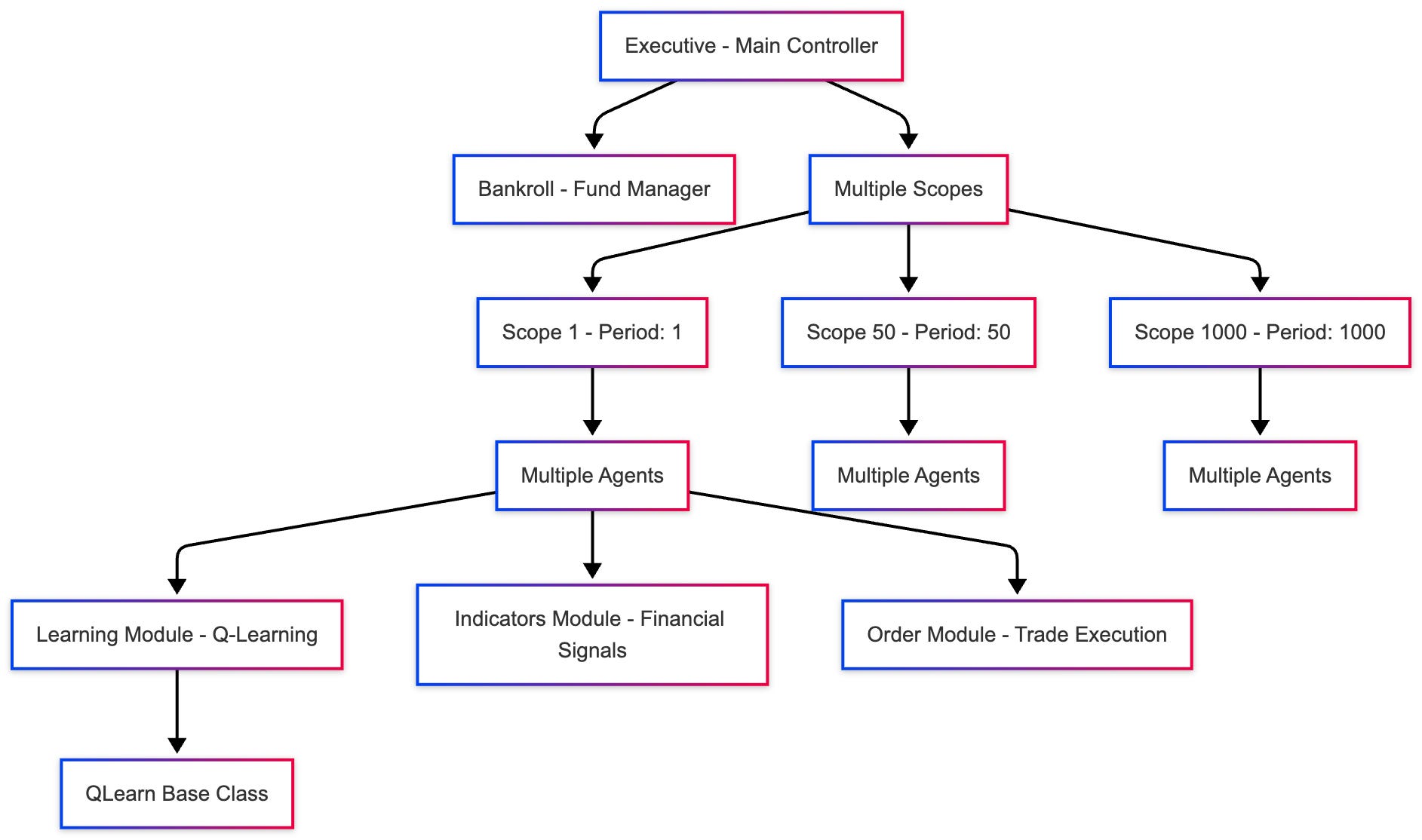
Architecture: Multi-agent system with scope-based trading
Core Concept: Scopes
The system uses an innovative concept called Scopes, which represents different time resolutions for analyzing market data.
What is a Scope? A sampling of time series quotes to discover trends along different time intervals
Purpose: At every moment, the system ensures at least one Agent per scope is looking for profitable trading opportunities
Default Scopes:
{1, 50, 1000}- meaning the system operates at three different time scales simultaneously
This multi-resolution approach allows the system to capture both short-term fluctuations and long-term trends.
System Architecture
Trading Loop (One “Hop”)
Individual Files
bankroll.py
Bankroll Module
The Bankroll module serves as the financial bookkeeping heart of the QuantScope trading system. This elegant yet powerful class manages all monetary transactions, maintains the current fund balance, and provides comprehensive logging of every financial operation that occurs during the trading simulation. Think of it as the central bank vault that meticulously tracks every dollar that flows in and out of the trading system, ensuring complete transparency and accountability for all trading activities.
The Bankroll class is instantiated once at the beginning of the trading simulation with an initial capital allocation. From that moment forward, it becomes the single source of truth for the system’s financial state. Every agent that wishes to open a position must deduct funds from the Bankroll, and every closed position that yields profit or loss must report back to the Bankroll. This centralized approach ensures that the system never loses track of its financial position and can immediately detect if trading activities have depleted the available capital.
Class Definition and Purpose
The Bankroll class encapsulates all fund management logic within a self-contained unit. It maintains three critical pieces of state: the current bankroll amount representing available capital, a transaction counter that assigns unique identifiers to each financial operation, and a dedicated logger that records every transaction to a separate log file for real-time monitoring and post-simulation analysis.
What makes this module particularly valuable is its dual-purpose design. Not only does it serve as a passive record-keeper, but it also acts as an active safety mechanism. By raising an exception when the bankroll goes negative, it immediately halts trading operations if the system runs out of money, preventing the simulation from continuing with invalid negative capital that would distort learning and analysis.
Constructor Method
def __init__(self, vault, funds):
self.init_logging(vault)
self.bankroll = funds
self.transactions = 0
self.logger.info(’Bankroll initialized with $ {}’.format(funds))
The constructor method initializes a new Bankroll instance and sets up the foundational infrastructure for fund management. When called, it accepts two parameters: the vault parameter specifies the file path where transaction logs should be written, while the funds parameter establishes the starting capital for the trading simulation.
The first action taken by the constructor is to invoke the `init_logging` method, passing the vault file path. This critical step establishes the logging infrastructure before any financial operations can occur, ensuring that even the initialization event itself can be recorded. Once logging is configured, the method stores the initial funds in the `self.bankroll` instance variable, which will be modified throughout the simulation as trading profits and losses accumulate.
The transaction counter `self.transactions` begins at zero, ready to be incremented with each financial operation. Finally, the constructor logs an informational message announcing the initialization and documenting the starting capital amount. This creates an auditable record showing exactly how much money the system began trading with, which becomes crucial when analyzing final performance metrics.
Transaction Method
def transaction(self, val):
self.bankroll += val
self.transactions += 1
self.logger.info(’Transaction {id}: $ {val} added to bankroll: $ {br}’\
.format(id=self.transactions, val=val, br=self.bankroll))
if self.bankroll < 0:
raise Exception(’We ran out of money’)
The transaction method represents the core operational function of the Bankroll class, handling every monetary movement that occurs during trading. This method is called whenever an agent opens or closes a position, with the val parameter carrying either a negative value when funds are being spent to open a position, or a positive value when proceeds from closing a position are being returned.
When invoked, the method first updates the bankroll by adding the transaction value. For opening positions, this represents a deduction since the value is negative, reducing available capital by the amount needed to purchase the currency position. For closing positions, this adds the proceeds back to the available funds, which may be more or less than what was originally spent depending on whether the trade was profitable.
Immediately after updating the balance, the method increments the transaction counter. This serves multiple purposes: it provides a unique identifier for each transaction making it easier to trace specific operations in the logs, it allows the system to calculate the total number of trades executed, and it helps correlate transactions with agent activities when analyzing system behavior.
The logging statement that follows creates a detailed record of the transaction. It captures the transaction ID, the amount added or subtracted (which could be negative), and the resulting bankroll balance after the transaction completes. This three-part record allows someone monitoring the `bankroll.log` file to see the complete story of each financial operation: which transaction number it was, how much money moved, and what the new total balance became. The format string clearly shows these relationships, making the log file human-readable for real-time monitoring.
The final component of this method implements a critical safety mechanism. After every transaction, the code checks whether the bankroll has fallen below zero. If this condition is detected, meaning the system has attempted to trade with more money than it possesses, the method immediately raises an exception with the message “We ran out of money.” This exception propagates up through the call stack and halts the entire simulation, preventing the system from continuing to operate in an invalid financial state. This safeguard ensures that the Q-learning algorithm never learns from scenarios where the agent traded with capital it didn’t actually have, which would corrupt the learning process and invalidate the simulation results.
Get Bankroll Method
```python
def get_bankroll(self):
return self.bankroll
```
The `get_bankroll` method provides a simple but essential accessor function that allows other components of the system to query the current financial state without directly accessing the internal `self.bankroll` variable. While this method appears trivial at first glance, consisting of just a single return statement, it embodies an important principle of object-oriented design: encapsulation.
By providing this dedicated method for reading the bankroll value, the class maintains control over how its internal state is accessed. Other system components, particularly the Executive class that needs to report the current bankroll in its logging statements, call this method to retrieve the current balance. This approach allows the Bankroll class to potentially add additional logic in the future, such as calculating interest, applying fees, or adjusting for currency conversions, without requiring changes to any code that reads the bankroll value.
The method is called frequently during the simulation’s main loop. At the beginning of each “hop” (the system’s term for a single step through the historical quote data), the Executive calls `get_bankroll()` to include the current financial state in its status logging. This creates a historical record of how the bankroll evolves over time, making it easy to visualize the system’s profitability trajectory and identify periods of strong or weak performance.
Logging Initialization Method
```python
def init_logging(self, log_file):
self.logger = logging.getLogger(’bankroll’)
self.logger.setLevel(logging.INFO)
fh = logging.FileHandler(log_file, mode=’w’)
fh.setLevel(logging.INFO)
ch = logging.StreamHandler()
ch.setLevel(logging.ERROR)
formatter = logging.Formatter(’%(asctime)s - %(name)s - %(levelname)s ‘\
‘- %(message)s’)
fh.setFormatter(formatter)
ch.setFormatter(formatter)
self.logger.addHandler(fh)
self.logger.addHandler(ch)
```
The `init_logging` method establishes the sophisticated logging infrastructure that makes the Bankroll’s operations transparent and auditable. This method is called exclusively by the constructor and sets up a dual-output logging system that writes to both a file and the console, though with different filtering levels for each destination.
The method begins by creating a named logger instance using Python’s logging framework, specifically requesting a logger with the name ‘bankroll’. This naming is significant because it allows the logging system to distinguish Bankroll transactions from other system logs, and it enables different configuration for this specific logger compared to others in the application. The logger’s base level is set to INFO, meaning it will process any message at INFO level or higher severity.
Next, the method creates a FileHandler pointing to the log file path provided in the log_file parameter. This handler is configured to open the file in write mode (‘w’), which means each time the simulation runs, it starts with a fresh log file, overwriting any previous results. The file handler’s level is set to INFO, ensuring that all informational messages about transactions and initialization will be written to the file. This creates the detailed transaction record that users can monitor in real-time using the `tail -f` command.
The method then establishes a second output channel: a StreamHandler that writes to the console (standard error stream). Interestingly, this handler’s level is set to ERROR rather than INFO. This design choice means that normal transaction operations won’t clutter the console output, but if something goes seriously wrong — such as the bankroll going negative — those critical error messages will appear on the console where they’re immediately visible to anyone running the simulation.
A unified formatter is created and applied to both handlers. This formatter specifies that each log entry should include the timestamp of when the event occurred, the name of the logger (‘bankroll’), the severity level of the message (INFO, ERROR, etc.), and finally the actual message content. This standardized format makes it easy to parse log files programmatically or scan them visually, as every entry follows the same predictable structure.
Finally, both handlers are attached to the logger instance. From this point forward, whenever code calls `self.logger.info()` or other logging methods, the message flows through this configured logger and gets written to both destinations according to their respective filtering levels. This dual-stream approach provides both a permanent detailed record (the file) and immediate visibility of critical issues (the console), making the system both observable during execution and analyzable after completion.
Role in the Trading System
The Bankroll module operates as the financial foundation upon which the entire QuantScope trading system is built. When the Executive class initializes the simulation, one of its first actions is to create a Bankroll instance with the configured starting capital, typically one thousand dollars. This Bankroll object is then passed as a reference to every Scope that gets created, and subsequently to every Agent that gets spawned within those scopes.
This shared reference pattern means that all agents across all scopes are accessing and modifying the same single Bankroll instance. When an agent in Scope 1 opens a buy position, it calls the Bankroll’s transaction method with a negative value representing the cost of the purchase. Microseconds later, an agent in Scope 50 might close a sell position and call the same Bankroll’s transaction method with a positive value representing the proceeds. Both operations modify the same underlying balance, maintaining a single source of truth for the system’s financial state.
The real-time logging capability of the Bankroll makes the trading system remarkably transparent. Users can open a terminal window, run the `tail -f logs/bankroll.log` command, and watch money flow in and out as the simulation progresses. Each line in this log represents an actual trading decision made by a learning agent, the financial consequences of that decision, and the cumulative effect on the system’s wealth. This visibility is invaluable for understanding how the Q-learning algorithm is performing and whether the agents are successfully learning profitable trading strategies.
The safety mechanism that halts execution when funds are depleted serves a dual purpose. On one level, it prevents the simulation from continuing with nonsensical negative capital, which would make the results meaningless. On another level, it provides immediate feedback about the algorithm’s effectiveness. If the simulation consistently runs out of money early in the process, it indicates that the agents are making poor trading decisions and the Q-learning parameters may need adjustment. Conversely, if the simulation completes with a healthy positive bankroll, it demonstrates that the agents successfully learned to trade profitably within the constraints of the historical data.
The transaction counter maintained by the Bankroll also provides valuable metrics. At the end of a simulation run, the total number of transactions indicates how actively the system traded. Combined with the final bankroll amount, this allows calculation of average profit per trade, which helps evaluate the quality of the learning algorithm’s decisions beyond just the final capital amount.
Executive Module
Overview
The Executive module serves as the master orchestrator and supreme commander of the entire QuantScope algorithmic trading system. This class sits at the apex of the system’s hierarchy, wielding complete control over the simulation lifecycle from initialization through execution to completion. The Executive is responsible for loading historical market data, establishing the financial infrastructure, creating and managing multiple trading scopes, and conducting the primary trading loop that drives the entire simulation forward through time.
When you run QuantScope by executing python python/executive.py, the Executive class springs into action as the entry point of the application. It coordinates the complex interplay between data loading, scope initialization, agent creation, and the continuous flow of market quotes through the system. Think of the Executive as a symphony conductor who doesn’t play any instrument directly but ensures that all musicians (in this case, scopes and agents) receive their cues at precisely the right moments and perform in perfect harmony to create profitable trading strategies.
The design philosophy of the Executive embodies the principle of centralized control with distributed execution. While the Executive maintains tight control over the simulation’s overall flow and timing, it delegates the actual trading decisions to autonomous agents operating within their respective scopes. This separation of concerns creates a clean architecture where strategic oversight remains distinct from tactical trading operations.
Module Constants and Configuration
QUOTES_CSV = ‘data/DAT_NT_USDCAD_T_LAST_201601.csv’
LOG_FILE = ‘logs/runlog.log’
VAULT = ‘logs/bankroll.log’
FUNDS = 1000
SCOPES = {1, 50, 1000}
Q = dict()
ALPHA = 0.7
REWARD = tuple()
DISCOUNT = 0.314
LIMIT = 11
Before the Executive class itself is even defined, the module establishes a collection of configuration constants that govern the simulation’s behavior. These constants represent the fundamental parameters that determine how the trading system operates, and modifying them allows users to experiment with different trading strategies and learning configurations without altering the core algorithmic logic.
The QUOTES_CSV constant specifies the file path to the historical market data that will feed the simulation. This CSV file contains thousands of CAD/USD forex quotes from January 2016, providing the raw material upon which the agents will learn to trade. The LOG_FILE constant designates where the Executive should write its detailed execution logs, capturing the progression of the simulation and the current state of the system at each step. The VAULT constant points to the Bankroll’s dedicated transaction log file, creating a separation between general system logging and specific financial transaction records.
The FUNDS constant establishes the starting capital for the trading simulation, set at one thousand dollars. This initial bankroll represents the financial resources that all agents across all scopes will share, compete for, and hopefully grow through successful trading. The SCOPES constant defines the set of time resolutions at which the system will operate simultaneously. The values {1, 50, 1000} mean the system will maintain three parallel perspectives on the market: a high-frequency view that updates every quote, a medium-frequency view that updates every fifty quotes, and a low-frequency view that updates every thousand quotes. This multi-scale approach allows the system to capture both rapid price movements and longer-term trends.
The Q constant initializes an empty dictionary that will eventually hold the Q-learning table shared across all agents. This shared knowledge base allows agents to benefit from each other’s experiences. The ALPHA constant sets the learning rate for the Q-learning algorithm at 0.7, determining how aggressively the agents update their knowledge based on new trading outcomes. A higher alpha means the agents adapt more quickly to recent experiences, while a lower value creates more stable but slower learning.
The REWARD tuple, though initialized as empty here, represents the reward structure that will guide the Q-learning process. The DISCOUNT constant, set to 0.314, determines how much the agents value future rewards compared to immediate ones. This particular value suggests that the system prioritizes relatively near-term profits rather than distant speculative gains. Finally, the LIMIT constant caps the number of agents that can exist within any single scope at eleven, preventing the system from spawning unlimited agents and consuming unbounded computational resources.
Constructor Method
def __init__(self):
self.init_logging()
self.logger.info(’Initializing Executive...’)
self.bankroll = Bankroll(VAULT, FUNDS)
self.all_quotes = []
self.quotes = []
self.scopes = []
self.load_csv()
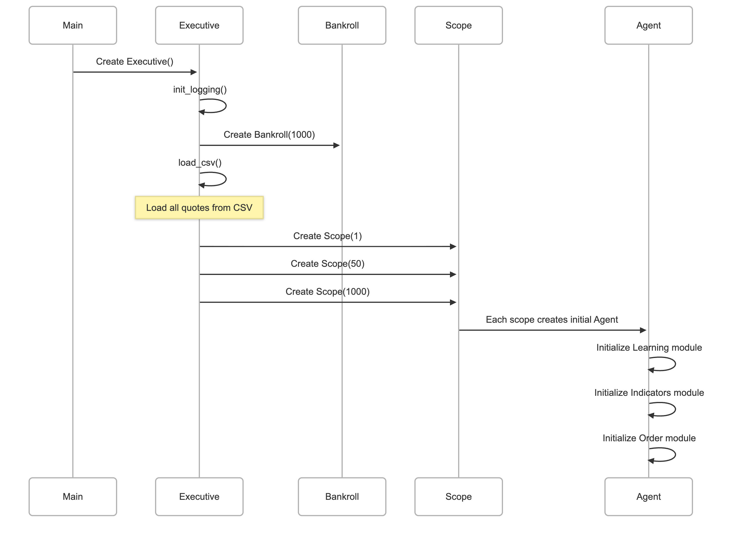
self.load_scopes()The constructor method orchestrates the complete initialization sequence that transforms an empty Executive instance into a fully operational trading system ready to begin simulation. This method executes a carefully ordered series of setup steps, each building upon the foundation laid by the previous operations.
The first action taken is calling self.init_logging(), establishing the logging infrastructure before any other operations occur. This priority ensures that every subsequent action can be properly recorded, creating a complete audit trail from the very beginning of initialization. Once logging is active, the constructor immediately logs an informational message announcing that Executive initialization has begun, creating a clear marker in the log files that delineates the start of a new simulation run.
Next, the constructor creates the Bankroll instance that will serve as the financial backbone of the trading system. By passing the VAULT file path and FUNDS amount to the Bankroll constructor, the Executive establishes centralized fund management with the configured starting capital. This Bankroll object becomes a shared resource that will be passed to all scopes and subsequently to all agents, ensuring that every trading operation affects the same single source of financial truth.
The method then initializes three empty list structures that will hold critical data throughout the simulation. The self.all_quotes list will store the complete historical dataset loaded from the CSV file, representing the full universe of market data available for the simulation. The self.quotes list will accumulate quotes progressively as the simulation advances, representing the subset of historical data that agents have “seen” up to the current simulation point. This separation between all available data and currently visible data is crucial for realistic backtesting, as it prevents agents from inadvertently learning from future data. The self.scopes list will hold the Scope objects that contain the trading agents, forming the primary operational structure of the system.
With these data structures in place, the constructor calls self.load_csv() to populate self.all_quotes with historical market data from the specified CSV file. This operation reads potentially millions of data points and prepares them for sequential processing during the simulation. Finally, the constructor invokes self.load_scopes() to create the multi-resolution scope structure. This method instantiates separate Scope objects for each configured time resolution, with each scope receiving references to the shared Q-learning table, the common Bankroll, and the simulation’s logger. At this point, initialization is complete, and the Executive instance stands ready to begin the actual trading simulation.
Supervision Method
def supervise(self):
    self.logger.info(’Running...’)
    hop = 0
    while hop < len(self.all_quotes):
        self.logger.info(’Hop {hop} Bankroll: {bankroll}’.format(hop=hop,
                                     bankroll=self.bankroll.get_bankroll()))
        new_quote = self.get_new_quote(hop)
        for scope in self.active_scopes(hop):
            scope.refresh(new_quote)
            scope.trade()
        hop += 1
The supervise method represents the beating heart of the QuantScope trading system, implementing the primary execution loop that drives the simulation forward through historical time. This method transforms static market data into a dynamic trading environment where agents can learn from their decisions and evolve their strategies.
The method begins by logging a simple “Running…” message, marking the transition from initialization to active trading. It then initializes a hop counter to zero. In QuantScope terminology, a “hop” represents a single discrete step through the historical quote data, analogous to a single tick of a clock advancing the simulation forward in time. The hop counter will increment with each iteration of the main loop, tracking the simulation’s progress through the dataset.
The while loop continues executing as long as the hop counter remains less than the total number of quotes in the dataset. This means the simulation will process every single quote in the historical data, giving the agents maximum exposure to varied market conditions. On each iteration, the method first logs the current hop number along with the current bankroll balance. This creates a historical record that allows analysts to see how the system’s wealth evolves over time and correlate financial performance with specific points in the market data.
The next step retrieves a new quote by calling self.get_new_quote(hop), which extracts the quote corresponding to the current hop position from the all_quotes dataset and adds it to the growing quotes list that agents can access. This progressive revelation of data maintains the temporal integrity of the simulation, ensuring agents only trade based on information that would have been available at that point in historical time.
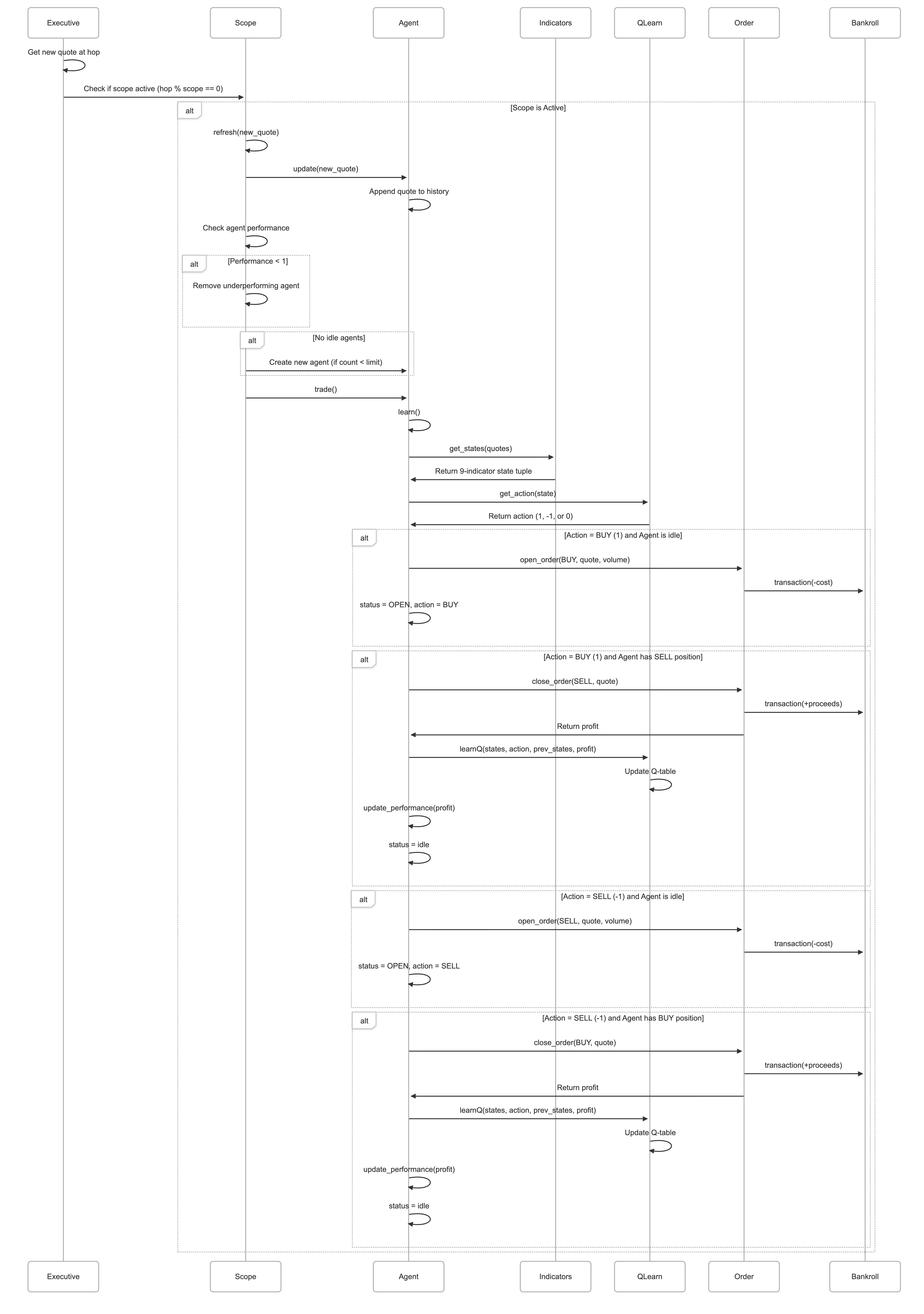
With the new quote in hand, the method enters a for loop that iterates over active scopes for the current hop. Not all scopes activate on every hop; the active_scopes() generator method yields only those scopes whose time resolution aligns with the current hop number. For example, Scope 1 activates every hop, Scope 50 activates every fiftieth hop, and Scope 1000 activates every thousandth hop. This selective activation implements the multi-timescale trading strategy that distinguishes QuantScope from simpler single-resolution systems.
For each active scope, the method calls two critical methods in sequence. First, scope.refresh(new_quote) updates all agents within that scope with the new market data, removes underperforming agents whose trading results have fallen below acceptable thresholds, and spawns new agents if necessary to maintain adequate trading capacity. Second, scope.trade() triggers all agents within the scope to analyze the current market state and execute trading decisions based on their learned Q-learning policies. These two operations—refresh and trade—constitute the core cycle of observation, learning, and action that enables the reinforcement learning process.
After processing all active scopes for the current hop, the loop increments the hop counter and continues to the next iteration. This process repeats thousands or potentially millions of times until every quote in the historical dataset has been processed, at which point the while loop terminates and the simulation concludes. The final state of the bankroll at this point represents the cumulative result of all trading decisions made by all agents across all scopes throughout the entire simulation.
Active Scopes Generator
def active_scopes(self, hop):
    “”“
    Generator of active scopes for a given hop.
    “”“
    for scope in self.scopes:
        if hop % scope.scope == 0:
            yield scope
The active_scopes method implements a clever generator function that determines which scopes should process trading logic at any given hop in the simulation. This method embodies the multi-timescale strategy that forms the conceptual foundation of QuantScope’s trading approach.
The method accepts a single parameter representing the current hop number and uses Python’s generator syntax (the yield keyword) to create an iterator that produces scopes on demand rather than building a complete list in memory. This lazy evaluation approach is computationally efficient, particularly as the method is called once per hop throughout the potentially lengthy simulation.
The implementation iterates through all scopes stored in self.scopes and applies a simple but powerful modulo test to each one. The expression hop % scope.scope == 0 checks whether the current hop number is evenly divisible by the scope’s resolution value. For Scope 1, this condition is always true since any number modulo 1 equals zero. For Scope 50, the condition is true only on hops 0, 50, 100, 150, and so on. For Scope 1000, it’s true only on hops 0, 1000, 2000, and so forth.
This elegant mathematical approach creates the temporal stratification that allows the system to simultaneously operate at multiple frequencies. On most hops, only Scope 1 is active, allowing high-frequency agents to respond to every market fluctuation. On every fiftieth hop, both Scope 1 and Scope 50 activate, adding medium-frequency perspective to the trading decisions. On every thousandth hop, all three scopes activate simultaneously, creating a moment where short-term, medium-term, and long-term strategies all process the same market data and potentially execute coordinated trades.
The generator yields each active scope as soon as it’s identified, allowing the supervise method to begin processing that scope immediately rather than waiting for all active scopes to be identified. This streaming approach maintains the temporal flow of the simulation and aligns with the philosophy of incremental, just-in-time processing that pervades the architecture.
Load Scopes Method
def load_scopes(self):
    for scope in SCOPES:
        self.scopes.append(Scope(scope, Q, ALPHA, REWARD, DISCOUNT, LIMIT,
                                   self.quotes, self.bankroll, self.logger))
    self.logger.info(’Scopes generated’)
The load_scopes method constructs the multi-resolution scope structure that will house the trading agents throughout the simulation. This initialization step creates the organizational framework within which autonomous learning and trading will occur.
The method iterates through the SCOPES set, which by default contains the values {1, 50, 1000}, representing three different temporal resolutions for market analysis. For each scope value, the method instantiates a new Scope object, passing a comprehensive set of parameters that connect the scope to the broader system infrastructure.
The first parameter is the scope value itself, which determines the temporal frequency at which this scope will activate. The second parameter is the shared Q-learning dictionary that allows all agents across all scopes to learn from each other’s experiences. By passing the same dictionary reference to every scope, the system creates a collective learning environment where knowledge discovered by one agent immediately becomes available to all others.
The ALPHA parameter establishes the learning rate for Q-learning updates, controlling how aggressively agents modify their policies based on trading outcomes. The REWARD parameter, though currently an empty tuple, provides the framework for defining what constitutes success in trading. The DISCOUNT parameter determines the temporal preference of the learning algorithm, defining how much agents value future profits relative to immediate gains.
The LIMIT parameter caps the maximum number of agents that can exist within each scope, preventing unbounded agent proliferation that could consume excessive computational resources or create unwieldy complexity. The self.quotes reference provides each scope with access to the progressively growing list of observed market data. The self.bankroll reference connects all scopes to the shared financial resource, ensuring that every trading operation affects the same central pool of capital. Finally, the self.logger reference allows scopes and their agents to contribute to the unified logging stream, maintaining a coherent record of system behavior.
Each newly created Scope object is appended to the self.scopes list, building the collection that the supervise method will iterate through during the main trading loop. After all scopes have been created and stored, the method logs an informational message confirming that scope generation has completed successfully. At this point, the multi-resolution scope structure is fully established, and each scope contains at least one initial agent ready to begin learning and trading.
Get New Quote Method
def get_new_quote(self, x):
    new_quote = self.all_quotes[-x]
    self.quotes.append(new_quote)
    self.logger.info(’Quotes fetched’)
    return new_quote
The get_new_quote method implements the mechanism by which historical market data flows into the active trading simulation. This deceptively simple method handles the critical task of progressively revealing market data to agents in a temporally consistent manner that preserves the integrity of the backtesting process.
The method accepts a single parameter x, which represents the current hop number in the simulation. The first operation uses negative indexing to extract a quote from the all_quotes list. The expression self.all_quotes[-x] accesses the quote at position x from the end of the list. When x is 1, this retrieves the last quote in the dataset. When x is 2, it retrieves the second-to-last quote, and so on.
This reverse indexing creates an interesting temporal flow: the simulation actually processes the historical data in reverse chronological order, starting from the most recent quote and working backward toward the oldest. While this might seem counterintuitive at first, it doesn’t affect the learning process since the agents only see the progressively growing quotes list, which accumulates in forward chronological order regardless of how quotes are extracted from all_quotes.
After retrieving the new quote, the method appends it to the self.quotes list. This list represents the subset of historical data that has been “revealed” to the agents so far during the simulation. Each time get_new_quote is called, this list grows by one quote, gradually expanding the window of market data that agents can analyze when making trading decisions. This progressive revelation is crucial for realistic backtesting because it prevents agents from inadvertently using future information to inform past decisions, a common pitfall known as look-ahead bias.
The method logs an informational message indicating that quotes have been fetched. This creates a record in the log file marking each step of data ingestion, which can be useful for debugging or understanding the simulation’s progression. Finally, the method returns the newly retrieved quote to the calling code, allowing the supervise method to pass this fresh market data to the active scopes for processing.
Print Quotes Method
def print_quotes(self):
    for quote in self.all_quotes:
        print quote
The print_quotes method provides a simple utility function for examining the raw market data loaded from the CSV file. This method serves primarily as a debugging and inspection tool rather than a core operational component of the trading system.
The implementation iterates through every quote stored in the self.all_quotes list and prints each one to the console. This straightforward approach allows developers or analysts to visually inspect the market data, verify that the CSV loading process worked correctly, and understand the nature and range of the values being processed.
In practical usage, this method is rarely called during normal operation since printing potentially millions of quotes would overwhelm the console and provide little actionable information. However, during development, testing, or when troubleshooting data loading issues, this method offers a quick way to verify that the all_quotes list contains the expected data. A developer might temporarily call this method to spot-check a few quotes, confirm numerical formatting, or identify any anomalous values that might indicate data corruption or parsing errors.
The method represents good software engineering practice: providing simple inspection capabilities that aid development and debugging without adding unnecessary complexity to the primary operational logic.
Load CSV Method
def load_csv(self):
    with open(QUOTES_CSV) as csvfile:
        quotes = reader(csvfile, delimiter=’;’, quotechar=’|’)
        for quote in quotes:
             self.all_quotes.append(float(quote[-2]))
        self.logger.info(’Loading data complete’)
The load_csv method handles the critical task of reading historical market data from the persistent CSV file and transforming it into the in-memory data structure that will feed the trading simulation. This method bridges the gap between static file storage and dynamic runtime data structures.
The method begins by opening the file specified in the QUOTES_CSV constant using Python’s context manager syntax (the with statement). This approach ensures that the file will be properly closed even if an error occurs during processing, preventing resource leaks and file handle exhaustion. The file path points to a semicolon-delimited CSV file containing USD/CAD forex quotes from January 2016.
With the file open, the method creates a CSV reader object configured to parse the file’s specific format. The delimiter parameter specifies that fields are separated by semicolons rather than the more common commas, while the quotechar parameter indicates that pipe characters enclose fields that might contain delimiter characters. These parameters must match the actual format of the CSV file for parsing to succeed.
The method then enters a for loop that iterates through each row returned by the CSV reader. Each row represents a single quote record from the historical data. The expression quote[-2] accesses the second-to-last field in each row, which apparently contains the actual price value of interest. The negative indexing approach makes the code robust to rows with varying numbers of fields, as it always selects the penultimate field regardless of total field count.
The quote field is converted from its string representation to a floating-point number using the float() function, transforming textual data into numeric values suitable for mathematical operations. This numeric value is then appended to the self.all_quotes list, building a comprehensive collection of all market data points.
After processing every row in the CSV file, the loop completes and the with block closes the file automatically. The method concludes by logging an informational message confirming that data loading has finished successfully. At this point, self.all_quotes contains potentially hundreds of thousands or millions of quote values, ready to be progressively revealed to the trading agents during simulation.
The data loading process is performed once during initialization and the results are cached in memory throughout the simulation. This approach trades memory consumption for execution speed, allowing rapid access to quote data without repeatedly reading from disk during the time-critical simulation loop.
Logging Initialization Method
def init_logging(self):
    self.logger = logging.getLogger(’flow’)
    self.logger.setLevel(logging.DEBUG)
    fh = logging.FileHandler(LOG_FILE, mode=’w’)
    fh.setLevel(logging.DEBUG)
    ch = logging.StreamHandler()
    ch.setLevel(logging.INFO)
    formatter = logging.Formatter(’%(asctime)s - %(name)s - %(levelname)s ‘\
                                                            ‘- %(message)s’)
    fh.setFormatter(formatter)
    ch.setFormatter(formatter)
    self.logger.addHandler(fh)
    self.logger.addHandler(ch)
The init_logging method establishes the comprehensive logging infrastructure that makes the Executive’s operations visible and analyzable. This method creates a dual-output logging system that balances detailed record-keeping with manageable console output.
The method begins by obtaining a named logger instance from Python’s logging framework, specifically requesting a logger named ‘flow’. This naming creates a distinct logging channel for the Executive and related components, allowing the logging system to route and filter messages based on their source. The logger’s base severity level is set to DEBUG, the most verbose level, meaning this logger will process messages of any severity from DEBUG through INFO, WARNING, ERROR, and CRITICAL.
Next, the method creates a FileHandler configured to write logs to the file specified in the LOG_FILE constant. The mode parameter ‘w’ indicates write mode, which means each simulation run starts with a fresh log file, overwriting any previous execution logs. The file handler’s severity level is also set to DEBUG, ensuring that every log message generated by the Executive — regardless of how trivial — gets written to the file. This comprehensive file logging creates a complete audit trail of the simulation’s execution, invaluable for debugging unexpected behavior or analyzing the sequence of events during a trading session.
The method then establishes a second output channel by creating a StreamHandler that directs log messages to the console. Interestingly, this handler’s severity level is set to INFO rather than DEBUG. This design choice means that highly detailed DEBUG messages will appear in the log file but not clutter the console output. During a simulation run, users watching the console will see important informational messages about the system’s progress without being overwhelmed by granular debugging details. This filtered approach makes the console output useful for monitoring the simulation’s overall health without obscuring critical information beneath a flood of minutiae.
A unified formatter is created specifying the structure of log messages. Each entry will include the timestamp when the event occurred, the logger name (‘flow’), the severity level of the message, and the actual message content. This standardized format ensures consistency across all log entries, making it straightforward to parse log files programmatically or scan them visually to find specific events or track the progression of operations over time.
The formatter is applied to both the file handler and the console handler, ensuring that messages written to both destinations follow the same structural template. Finally, both handlers are registered with the logger instance. From this moment forward, whenever code calls self.logger.debug(), self.logger.info(), or other logging methods, those messages flow through this configured logger and get written to both the file and console according to their respective filtering rules.
Main Execution Block
if __name__ == “__main__”:
    trader = Executive()
    trader.supervise()
The main execution block at the bottom of the module implements the entry point for the QuantScope trading system. This simple two-line block transforms the executive.py file from a mere module definition into a runnable program.
The conditional if __name__ == “__main__” checks whether the Python interpreter is executing this file directly as a script rather than importing it as a module into another program. When you run python python/executive.py from the command line, Python sets the special __name__ variable to the string “main“, causing this conditional block to execute. If instead some other Python file imported executive.py to use its classes or functions, __name__ would be set to “executive” and this block would be skipped.
Inside the conditional, the first line instantiates a new Executive object, storing the reference in a variable named trader. This invocation triggers the entire initialization sequence implemented in the Executive’s constructor: logging setup, bankroll creation, data structure initialization, CSV loading, and scope generation. When this line completes, the trader object represents a fully initialized trading system ready to begin simulation.
The second line calls the supervise method on the newly created Executive instance. This invocation launches the main trading loop that will process the entire historical dataset, activating scopes at their designated frequencies and allowing agents to learn from their trading experiences. The supervise method will execute for an extended period — potentially minutes or hours depending on the dataset size and system performance — as it works through thousands or millions of market quotes.
When the supervise method finally completes after processing all historical data, control returns to the main execution block. Since there’s no code after the supervise call, the program terminates naturally, leaving behind log files that document the complete simulation run and a final bankroll value that quantifies the cumulative performance of all agents’ trading decisions.
Role in the Trading System
The Executive module occupies the commanding position at the apex of QuantScope’s hierarchical architecture. Every component of the system ultimately traces its origin to an Executive instance, and every trading operation ultimately occurs under the Executive’s oversight. When understanding QuantScope’s architecture, the Executive serves as the essential starting point because it orchestrates the creation and interaction of all other system components.
The Executive’s initialization sequence establishes the complete runtime environment for algorithmic trading. By loading historical data, creating the Bankroll, and instantiating multiple Scopes with their constituent Agents, the Executive transforms abstract configuration parameters into a functioning multi-agent learning system. The care taken to perform these initialization steps in the correct order — logging before operations, data loading before scope creation, scope creation before trading — ensures that each component has access to the resources it needs when it needs them.
During active trading, the Executive’s supervise method drives the entire system forward through simulated time. Its main loop represents the heartbeat of the simulation, pulsing once per quote to distribute new market data and trigger trading decisions. The Executive’s role in selectively activating scopes based on their temporal resolution implements the multi-timescale strategy that distinguishes QuantScope from simpler trading systems. By ensuring that high-frequency agents respond to every market movement while medium and low-frequency agents respond only at their designated intervals, the Executive orchestrates a complex symphony of trading activity operating at multiple temporal scales simultaneously.
The logging infrastructure established by the Executive creates visibility into the otherwise opaque process of multi-agent reinforcement learning. The detailed file logs capture every significant event during simulation, while the filtered console output provides real-time monitoring feedback. This dual-stream logging approach balances the needs of post-hoc analysis with the requirements of live monitoring, making the system both observable during execution and analyzable after completion.
The Executive’s clean separation of data loading, initialization, and execution phases exemplifies good software architecture. Each phase builds upon the previous one without creating circular dependencies or temporal paradoxes. The modular design means that future enhancements could modify data sources, add additional scopes, or alter the main loop’s structure without requiring wholesale rewrites of the entire system.
Indicators Module
Overview
The Indicators module serves as the analytical engine that transforms raw market price data into meaningful technical signals that guide trading decisions. This class implements a sophisticated suite of financial indicators drawn from classical technical analysis, each designed to detect specific patterns, trends, or market conditions that might predict future price movements. The Indicators module represents the “eyes” of the trading agents, distilling thousands of individual price quotes into a compact nine-dimensional state representation that captures the essential character of the current market environment.
Technical analysis operates on the principle that historical price patterns tend to repeat because they reflect consistent human psychology and market dynamics. The indicators implemented in this module detect these patterns through mathematical transformations of price data. Moving averages smooth out short-term noise to reveal underlying trends. The MACD (Moving Average Convergence Divergence) identifies momentum shifts by comparing moving averages at different timescales. The RSI (Relative Strength Index) measures the velocity and magnitude of price changes to identify overbought or oversold conditions. Together, these indicators provide a multi-faceted view of market state that forms the foundation for intelligent trading decisions.
The design of this module reflects a careful balance between analytical sophistication and computational efficiency. Each indicator returns a simple discrete signal (positive one, negative one, or zero) rather than a continuous numerical value. This discretization reduces the state space that the Q-learning algorithm must explore, making it feasible to learn effective trading policies from limited historical data. The nine-indicator tuple created by the get_states method represents a compressed encoding of market conditions that captures essential information while remaining computationally tractable for reinforcement learning.
Class Structure and Initialization
class Indicators(object):
    “”“
    This class defines financial indicators used to populate the state tuple.
    “”“
    def __init__(self, log=None):
        self.logger = log
        self.state = (0,0,0,0,0,0,0,0,0)
The Indicators class is designed as a mixin that will be inherited by the Agent class, allowing agents to seamlessly incorporate technical analysis capabilities into their decision-making process. The class structure follows object-oriented principles, encapsulating all indicator calculation logic within methods that operate on price quote data passed as parameters.
The constructor accepts an optional logger parameter that enables the indicators module to participate in the system’s comprehensive logging infrastructure. If a logger is provided, indicator calculations could theoretically log diagnostic information, though the current implementation focuses on silent computation rather than verbose logging. The logger reference is stored as an instance variable for potential future use by indicator methods that might need to record warnings about unusual market conditions or computational issues.
The initial state is set to a nine-element tuple of zeros, representing a neutral market condition where no indicators are signaling bullish or bearish patterns. This initialization ensures that the state variable always contains a valid tuple even before any actual indicator calculations have been performed. As agents begin analyzing market data, the get_states method will replace this neutral initial state with calculated values derived from actual price quotes.
The nine-dimensional structure of the state tuple is a critical design decision that defines the agent’s perception of the market. Each dimension corresponds to a specific indicator, and the position within the tuple is semantically meaningful. The Q-learning algorithm will learn to associate particular combinations of indicator values with successful trading outcomes, effectively discovering which patterns of technical signals predict profitable trading opportunities.
State Generation Method
def get_states(self, quotes):
    self.quotes = quotes
    self.state = (self.crossover_indicator(self.quotes, 5, 7),
                  self.crossover_indicator(self.quotes, 5, 20),
                  self.crossover_indicator(self.quotes, 7, 30),
                  self.crossover_indicator(self.quotes, 12, 26),
                  self.crossover_indicator(self.quotes, 50, 100),
                  self.crossover_indicator(self.quotes, 50, 200),
                  self.MACD_sig_line(self.quotes, 12, 26, 9),
                  self.MACD_zero_cross(self.quotes, 12, 26),
                  self.RSI(self.quotes, 14, 25))
    return self.state
The get_states method orchestrates the complete process of analyzing market data and generating the nine-dimensional state representation that agents use to make trading decisions. This method serves as the primary interface between raw price data and actionable market intelligence.
The method begins by storing the provided quotes parameter in self.quotes, making the price data available to all indicator calculation methods. This quotes parameter contains the complete historical sequence of prices that have been revealed to the agent up to the current simulation point, potentially spanning thousands of individual price observations. The growing size of this list over the course of the simulation means that early in the trading session, indicators have limited historical context, while later in the simulation they can detect longer-term patterns.
The core of the method constructs a nine-element tuple by calling various indicator calculation methods with carefully chosen parameters. The first six elements all use the crossover_indicator method but with different period combinations. The pairing of five and seven periods detects very short-term crossovers that might signal immediate trading opportunities. The pairing of five and twenty periods looks at slightly longer timeframes. The seven and thirty period combination extends the analysis further. The twelve and twenty-six period pairing aligns with standard MACD parameters, detecting medium-term momentum shifts. The fifty and one hundred period combination identifies major trend changes that might take weeks or months to develop in real market time. Finally, the fifty and two hundred period crossover, often called the “golden cross” in technical analysis, detects the most significant long-term trend reversals.
The seventh element invokes MACD_sig_line with the standard MACD parameters twelve and twenty-six for the MACD calculation, plus nine for the signal line averaging. This indicator specifically detects when the MACD line crosses its own moving average, a classic signal used by many technical traders. The eighth element calls MACD_zero_cross to detect when the MACD value itself crosses the zero line, indicating a shift from bearish to bullish momentum or vice versa.
The ninth and final element calculates the RSI using a fourteen-period lookback window and a threshold of twenty-five. This configuration means the RSI will signal oversold conditions (potential buying opportunities) when the index drops below twenty-five, and overbought conditions (potential selling opportunities) when it rises above seventy-five (since one hundred minus twenty-five equals seventy-five).
Each indicator returns either positive one (bullish signal), negative one (bearish signal), or zero (neutral or no clear signal). The resulting nine-element tuple encodes a comprehensive snapshot of market conditions across multiple timeframes and analytical perspectives. The Q-learning algorithm will learn to recognize which combinations of these nine values tend to precede profitable trading opportunities, effectively discovering patterns in the multidimensional indicator space that correlate with future price movements.
Moving Average Method
def moving_average(self, size, sliced):
    multiplier = 0.0
    multiplier = float((2/(float(size) + 1)))
    ema = sum(sliced)/float(size)
    for value in sliced:
        ema = (multiplier*value) + ((1-multiplier)*ema)
    if (ema == 0 and sum(sliced) != 0):
        print(”WE GOT A EMA PROBLEM MAWFUCKA”)
    return ema
The moving_average method implements the calculation of an Exponential Moving Average, a fundamental building block used by multiple higher-level indicators. The EMA differs from a simple moving average by giving greater weight to recent prices while still incorporating historical data, making it more responsive to current market conditions while maintaining stability.
The method accepts two parameters: size specifies the period length for the moving average calculation, while sliced contains the actual price data to be averaged. The sliced parameter typically contains the most recent N prices extracted from the full quote history, where N equals the size parameter.
The calculation begins by computing the smoothing multiplier used in the exponential weighting formula. The expression 2/(size + 1) represents the standard formula for EMA smoothing factors. For a twenty-period EMA, this yields approximately 0.095, meaning each new price contributes about nine and a half percent to the new average while the previous average contributes about ninety and a half percent. This exponential weighting creates the characteristic responsiveness of EMAs.
The method initializes the EMA with a simple average of all values in the sliced data. This seed value provides a starting point for the exponential averaging process. The subsequent for loop iterates through each price value, repeatedly applying the exponential weighting formula. Each iteration updates the EMA by blending the current price value (weighted by the multiplier) with the existing EMA value (weighted by one minus the multiplier).
The mathematical effect of this repeated application is subtle but important. Although the loop processes each value sequentially, the exponential weighting ensures that the final EMA value gives appropriate weight to all prices, with recent prices having greater influence. The iterative structure effectively implements the recursive formula that defines exponential moving averages: EMA_today = (Price_today × multiplier) + (EMA_yesterday × (1 — multiplier)).
The conditional statement at the end implements a sanity check to detect numerical anomalies. If the calculated EMA is exactly zero despite the input data having non-zero values, something has gone wrong in the calculation, possibly due to numerical underflow or data corruption. The colorful error message would alert developers to investigate the issue, though in practice with well-formed forex price data, this condition should never occur.
The method returns the calculated EMA value, which higher-level indicator methods will compare or combine to generate trading signals. The EMA serves as a smoothed representation of recent price history, filtering out random fluctuations while preserving genuine trends.
Crossover Indicator Method
def crossover_indicator(self, q, x, y):
    if self.moving_average(x, q[-x:]) < self.moving_average(y, q[-y:]):
        if self.moving_average(x, q[-x-1:-1]) > self.moving_average(y,
                                                                q[-y-1:-1]):
            return -1
    elif self.moving_average(x, q[-x:]) > self.moving_average(y, q[-y:]):
        if self.moving_average(x, q[-x-1:-1]) < self.moving_average(y,
                                                                q[-y-1:-1]):
            return 1
    return 0
The crossover_indicator method detects one of the most fundamental patterns in technical analysis: the moment when two moving averages of different periods cross each other, signaling a potential trend reversal or momentum shift. This method embodies the principle that comparing trends at different timescales can reveal important information about market direction.
The method accepts three parameters: q contains the complete quote history, while x and y specify the periods for the fast and slow moving averages respectively. Typically x is smaller than y, creating a fast MA that responds quickly to price changes and a slow MA that changes more gradually, though the method works correctly regardless of the relationship between x and y.
The implementation uses negative list slicing to extract the relevant price data for each moving average calculation. The expression q[-x:] extracts the last x elements from the quote list, providing the data window for the fast moving average. Similarly, q[-y:] extracts the last y elements for the slow moving average. These slices always capture the most recent prices, ensuring the moving averages reflect current market conditions.
The first condition checks whether the current fast MA is less than the current slow MA, indicating that the faster-moving trend is currently below the slower trend. If this condition is true, the nested conditional checks whether the previous fast MA (calculated from q[-x-1:-1]) was greater than the previous slow MA. This combination—fast below slow now, but fast above slow previously—indicates that the fast MA has just crossed below the slow MA, a bearish crossover that often precedes downward price movement. The method returns negative one to signal this bearish condition.
The complementary elif branch detects the opposite pattern: if the current fast MA exceeds the current slow MA, and the previous fast MA was below the previous slow MA, then a bullish crossover has just occurred. The fast MA crossing above the slow MA suggests strengthening upward momentum, and the method returns positive one to signal this bullish condition.
If neither crossover condition is met — meaning either the MAs haven’t crossed, or they crossed more than one step ago — the method returns zero, indicating no actionable signal. This three-valued output (negative one, zero, positive one) fits perfectly into the discrete state space used by the Q-learning algorithm.
The use of both current and previous MA values is crucial for detecting crossovers specifically at the moment they occur. Simply comparing current MA values would indicate whether the fast MA is above or below the slow MA, but wouldn’t distinguish between a stable configuration that has persisted for many time steps versus a fresh crossover that just happened. By requiring that the relationship has changed from the previous step, the method ensures signals are generated only at the precise moments when trends shift.
MACD Calculation Method
def MACD(self, q, m1, m2):
    signal = self.moving_average(m1, q[-m1:]) - self.moving_average(m2, q[-m2:])
    return signal
The MACD method implements the core calculation of the Moving Average Convergence Divergence indicator, one of the most widely used momentum indicators in technical analysis. The MACD measures the relationship between two exponential moving averages of different periods, revealing the strength and direction of market momentum.
The method accepts three parameters: q contains the quote history, while m1 and m2 specify the periods for the two moving averages that will be compared. In standard MACD configuration, m1 is twelve and m2 is twenty-six, representing roughly two weeks and one month of trading data respectively in daily price charts. These particular values have become conventional through decades of practical use, though the periods can be adjusted for different market conditions or trading timeframes.
The calculation itself is elegantly simple: subtract the longer-period moving average from the shorter-period moving average. When prices are rising, the twelve-period EMA will typically be above the twenty-six period EMA, producing a positive MACD value. When prices are falling, the twelve-period EMA will typically be below the twenty-six-period EMA, producing a negative MACD value. The magnitude of the MACD value indicates the strength of the trend — larger absolute values suggest stronger momentum in the corresponding direction.
The genius of the MACD lies in what it reveals about momentum dynamics. When the MACD value is positive and increasing, it indicates not only that prices are above their longer-term average, but that the gap is widening, suggesting accelerating upward momentum. When the MACD is positive but decreasing, prices are still above the longer-term average but the momentum is weakening, possibly signaling an upcoming reversal. The negative MACD values reveal the corresponding patterns for downward trends.
This method returns the raw MACD value, which other indicator methods will analyze further. The MACD_sig_line method will compare this value to a moving average of MACD values to detect crossovers. The MACD_zero_cross method will compare it to zero to detect momentum reversals. The modular design allows the basic MACD calculation to be reused by multiple higher-level indicators without code duplication.
MACD Series Method
def MACD_series(self, q, m1, m2):
    series = []
    i = 0
    for quotes in q:
        if m2 > i:
            series.append(self.moving_average(m1, q[-m1-i:-i]) - self.moving_average(m2, q[-m2-i:-i]))
        i += 1
    if m2 < i:
        series.append(self.MACD(q,m1,m2))
    return series
The MACD_series method generates a historical sequence of MACD values computed at different points in the quote history. This series of MACD values is essential for calculating the MACD signal line, which is itself a moving average of MACD values. The method constructs a time series that shows how the MACD indicator has evolved over recent market history.
The method accepts three parameters: q contains the full quote history, while m1 and m2 are the MACD periods that will be used for each calculation. The method initializes an empty list to accumulate MACD values and a counter i to track position within the historical data.
The for loop iterates through each quote in the history, though interestingly it doesn’t actually use the individual quote values from the iteration variable. Instead, the loop serves primarily to advance the counter i. On each iteration, the conditional checks whether m2 (typically twenty-six) exceeds i. When this condition is true, meaning we haven’t yet processed enough iterations to equal the longer MACD period, the method calculates a historical MACD value using backward-looking slices.
The slice expressions q[-m1-i:-i] and q[-m2-i:-i] extract historical windows of data positioned i steps back from the most recent quote. When i is zero, these slices capture the most recent data. When i is one, they capture data ending one quote before the most recent. As i increases, the windows slide progressively further into the past, calculating MACD values as they would have appeared at each historical moment.
After the loop completes, the final conditional checks if we’ve processed enough iterations to exceed the longer MACD period. If so, it appends one more MACD value calculated from the most current data using the standard MACD method. This ensures the series includes a MACD value for the current market moment in addition to the historical values.
The resulting series list contains MACD values calculated at successive points in market history, with each value representing what the MACD indicator showed at that particular moment. This historical series allows the MACD_sig_line method to compute a moving average of recent MACD values, creating the signal line that traders use to identify MACD crossovers.
The implementation reflects the recursive nature of technical analysis: we compute moving averages of prices, then compute the MACD as a difference of moving averages, then compute a series of historical MACD values, and finally (in other methods) compute a moving average of those MACD values. Each layer of abstraction reveals different aspects of market structure and momentum.
MACD Signal Line Method
def MACD_sig_line(self, q, m1, m2, m3):
    self.series = self.MACD_series(q, m1, m2)
    if self.MACD(q, m1, m2) < self.moving_average(m3, self.series[-m2:]):
        if self.MACD(q[:-1], m1, m2) > self.moving_average(m3, self.series[-m2-1:-1]):
            return -1
    elif self.MACD(q, m1, m2) > self.moving_average(m3, self.series[-m2:]):
        if self.MACD(q[:-1], m1, m2) < self.moving_average(m3, self.series[-m2-1:-1]):
            self.series = self.MACD_series(q, m1, m2)
    if self.MACD(q, m1, m2) < self.moving_average(m3, self.series[-m2:]):
        if self.MACD(q[:-1], m1, m2) > self.moving_average(m3, self.series[-m2-1:-1]):
            return -1
    elif self.MACD(q, m1, m2) > self.moving_average(m3, self.series[-m2:]):
        if self.MACD(q[:-1], m1, m2) < self.moving_average(m3, self.series[-m2-1:-1]):
            return 1
    return 0
The MACD_sig_line method detects crossovers between the MACD line and its signal line, one of the most popular trading signals in technical analysis. The signal line is simply a moving average of recent MACD values, and crossovers between the MACD and this smoothed version often precede significant price movements.
The method accepts four parameters: q contains the quote history, m1 and m2 are the standard MACD periods (typically twelve and twenty-six), and m3 specifies the signal line period (typically nine). The method begins by generating the complete MACD series using the MACD_series method, creating a historical sequence of MACD values that can be averaged to produce the signal line.
The signal line itself is calculated using the moving_average method applied to the most recent m3 elements of the MACD series. This creates a smoothed version of the MACD that changes more gradually than the MACD line itself, similar to how the slow moving average in a crossover indicator changes more gradually than the fast moving average.
The detection logic follows the same pattern as the crossover_indicator method, but applied to MACD values instead of prices. The first conditional checks if the current MACD is below the current signal line, and if the previous MACD was above the previous signal line. This combination indicates a bearish crossover — the MACD has just crossed below its signal line — which often precedes downward price movement. The method returns negative one to signal this bearish condition.
The elif branch detects the complementary bullish crossover: current MACD above signal line, previous MACD below signal line. Interestingly, this branch includes a statement that recalculates the MACD series, though this appears to be redundant since the series was already calculated at the beginning of the method. This might represent a defensive programming practice or a vestige of earlier code versions.
The code then appears to repeat the same crossover detection logic again, checking for both bearish and bullish crossovers a second time. This duplication might seem unnecessary, but it could serve as a form of double-checking or handle edge cases where the series needs to be recalculated mid-method. In practice, if either set of conditionals detects a crossover, the method will return the appropriate signal value.
If no crossover is detected by any of the conditional branches, the method returns zero, indicating that either the MACD and signal line haven’t crossed, the crossover happened in a previous time step, or they’re moving in parallel. This neutral signal tells the Q-learning algorithm that the MACD indicator doesn’t currently provide actionable information for trading decisions.
The MACD signal line crossover is particularly valued by traders because it combines trend identification with momentum measurement. The MACD itself measures momentum, and the signal line smooths that momentum reading. When the raw momentum crosses above its smoothed version, it suggests not just that prices are rising, but that the rate of increase is accelerating, a strong bullish signal.
MACD Zero Cross Method
def MACD_zero_cross(self, q, m1, m2):
    if self.MACD(q[:-1], m1, m2) > 0 and self.MACD(q, m1, m2) < 0:
        return -1
    elif self.MACD(q[:-1], m1, m2) < 0 and self.MACD(q, m1, m2) > 0:
        return 1
    return 0
The MACD_zero_cross method detects when the MACD indicator crosses the zero line, a significant event in technical analysis that often indicates a fundamental shift in market momentum. Because the MACD represents the difference between two moving averages, a zero crossing means those moving averages have converged to equality, marking the transition point between bullish and bearish regimes.
The method accepts three parameters: q contains the quote history, while m1 and m2 specify the MACD calculation periods. The implementation is remarkably concise, calculating the MACD value for both the current market state and the previous market state, then comparing these values to zero to detect crossings.
The first conditional examines whether the previous MACD value was positive while the current MACD value is negative. This pattern indicates that the MACD has crossed from above zero to below zero, a bearish signal. When the twelve-period EMA falls below the twenty-six-period EMA, it suggests that recent price action has weakened relative to the longer-term trend. The method returns negative one to communicate this bearish zero crossing.
The elif branch detects the opposite scenario: previous MACD negative, current MACD positive. This bearish-to-bullish transition occurs when the twelve-period EMA rises above the twenty-six-period EMA, indicating that recent prices have strengthened relative to the longer-term average. This crossover from below zero to above zero is considered a bullish signal, and the method returns positive one.
If neither crossing condition is met, either because the MACD hasn’t crossed zero or because it crossed at some earlier time, the method returns zero to indicate no actionable signal. The zero return communicates to the Q-learning algorithm that this particular indicator doesn’t currently provide useful information for trading decisions.
The MACD zero crossing is considered more significant than arbitrary MACD value changes because it represents a clear structural shift in the relationship between short-term and long-term price trends. When the MACD is positive, short-term momentum exceeds long-term momentum, suggesting prices are in an uptrend. When the MACD is negative, the opposite is true. The crossing point marks the exact moment when this relationship inverts, making it a natural point to reconsider trading positions.
By detecting these zero crossings and encoding them as discrete signals in the state tuple, the method allows the Q-learning algorithm to learn whether MACD zero crossings reliably predict profitable trading opportunities in the specific market being analyzed. Some markets might show strong correlation between MACD crossings and future price movements, while others might not, and the learning algorithm will discover which patterns matter through experience.
Relative Strength Index Method
def RSI(self, q, period, threshold):
    i = 0
    upcount = 0
    downcount = 0
    RS = 50.0
    updays = []
    downdays = []
    while (upcount <= period and downcount <= period) and i < len(q) - 1:
        if q[1+i] < q[i]:
            updays.append(q[1+i])
            upcount += 1
        elif q[1+i] > q[i]:
            downdays.append(q[1+i])
            downcount += 1
        i += 1
    try:
        RS = self.moving_average(period, updays) / self.moving_average(period, downdays)
    except:
        RS = 0
    if float(self.moving_average(period, downdays)) != 0.0:
        RS = float(self.moving_average(period, updays)) / float(self.moving_average(period, downdays))
    RSI = (100-(100/(1+RS)))
    if RSI < threshold:
        return 1
    elif RSI > (100-threshold):
        return -1
    return 0
The RSI method implements the Relative Strength Index, a momentum oscillator that measures the velocity and magnitude of price changes to identify overbought or oversold conditions. The RSI was developed by J. Welles Wilder Jr. and has become one of the most widely used technical indicators for detecting potential reversal points.
The method accepts three parameters: q contains the quote history, period specifies how many price changes to analyze (typically fourteen), and threshold determines the boundary values that trigger overbought or oversold signals (typically twenty-five, creating thresholds at twenty-five and seventy-five on the zero-to-one-hundred RSI scale).
The method begins by initializing several variables that will accumulate data during the calculation process. The counter i tracks position in the quote history, while upcount and downcount track how many upward and downward price movements have been identified. The RS variable initializes to fifty, representing a neutral relative strength value. Two lists, updays and downdays, will accumulate the magnitudes of price increases and decreases respectively.
The while loop examines consecutive price pairs to classify each movement as either upward or downward. The loop continues until it has collected enough price movements to equal the specified period, or until it exhausts the available quote history. On each iteration, the code compares the price at position i+1 with the price at position i. If the later price is lower, this represents a price decrease, so the later price is appended to the updays list. Conversely, if the later price is higher, this represents a price increase, and the later price is appended to downdays.
This classification might seem counterintuitive at first — why does a price decrease contribute to “updays”? The answer lies in the RSI’s economic interpretation: the RSI measures the relative strength of buying versus selling pressure. When prices fall, it indicates selling pressure, and the magnitude of the price at that moment contributes to the calculation of average selling pressure. Similarly, rising prices indicate buying pressure. The naming reflects this interpretation rather than the literal direction of price movement.
After collecting price movements, the code calculates the Relative Strength ratio by dividing the moving average of upday prices by the moving average of downday prices. This ratio quantifies the balance between buying and selling pressure. A ratio greater than one means buying pressure exceeds selling pressure on average, while a ratio less than one indicates stronger selling pressure.
The try-except block handles the edge case where downdays might be all zeros or empty, which would cause division by zero. If such an error occurs, the RS is set to zero. The subsequent conditional provides a more explicit check for zero downdays average, recalculating the RS ratio only if the denominator is non-zero. This defensive programming ensures the method handles unusual market conditions gracefully without crashing.
The RSI value itself is calculated using the formula: RSI = 100 — (100 / (1 + RS)). This transformation maps the Relative Strength ratio (which ranges from zero to infinity) onto a bounded scale from zero to one hundred. When RS is very high (strong buying pressure), the RSI approaches one hundred. When RS is very low (strong selling pressure), the RSI approaches zero. An RS of one (balanced pressure) produces an RSI of fifty.
The final conditionals convert the continuous RSI value into a discrete trading signal based on the threshold parameter. If the RSI falls below the threshold (typically twenty-five), the market is considered oversold — prices have fallen so much that a reversal upward seems likely — and the method returns positive one to suggest buying. If the RSI exceeds one hundred minus the threshold (typically seventy-five), the market is considered overbought — prices have risen so much that a reversal downward seems likely — and the method returns negative one to suggest selling. If the RSI falls in the middle range between these extremes, the method returns zero, indicating the RSI doesn’t currently provide a clear signal.
The RSI’s effectiveness stems from the observation that extreme price movements often exhaust themselves and reverse. When the RSI indicates oversold conditions, it suggests that selling pressure has become excessive and a bounce upward is likely. Conversely, overbought conditions suggest buying pressure has become unsustainable and a correction downward is imminent. By encoding these conditions as discrete signals, the method allows the Q-learning algorithm to learn whether RSI extremes reliably predict profitable reversal trades in the specific market being analyzed.
Role in the Trading System
The Indicators module serves as the perceptual system for the entire QuantScope trading architecture. When an agent needs to decide whether to buy, sell, or hold, it calls get_states to transform the raw quote history into a structured representation of market conditions. This transformation is crucial because the Q-learning algorithm cannot directly process thousands of individual price quotes — it needs a compact state representation that captures the essential character of the market while fitting within a tractable state space for learning.
The nine indicators were chosen to provide complementary perspectives on market state. The six crossover indicators examine trends at progressively longer timeframes, from very short-term (five versus seven periods) to very long-term (fifty versus two hundred periods). This multi-resolution trend analysis ensures the agent considers both immediate price action and broader market context. The two MACD-based indicators add momentum analysis, detecting whether trends are accelerating or decelerating. The RSI adds a contrarian perspective, identifying moments when prices have moved too far too fast and might be due for reversal.
The discretization of indicator values into three-state signals (positive one, zero, negative one) represents a crucial design choice that balances expressiveness with learnability. Continuous indicator values would provide more nuanced information but would create an infinite state space that reinforcement learning algorithms struggle to explore effectively. The three-valued discretization creates a state space of three to the ninth power, roughly twenty thousand possible states — large enough to capture important market variations but small enough for the Q-learning algorithm to explore thoroughly and learn meaningful patterns.
The modular design of the Indicators class, with separate methods for moving averages, MACD calculations, and RSI computations, promotes code reuse and maintainability. The moving_average method serves as a fundamental building block used by multiple higher-level indicators. The MACD and MACD_series methods separate the basic MACD calculation from the series generation required for signal line analysis. This modularity makes it easy to add new indicators, modify existing ones, or experiment with different parameter values without creating code duplication or introducing bugs.
The careful handling of edge cases — checking for zero divisors in RSI, validating EMA calculations, using defensive conditionals — ensures the indicators module operates reliably even when confronted with unusual market conditions or limited historical data. This robustness is essential because the module processes millions of calculations throughout a typical simulation, and a single failure could corrupt the learning process or crash the entire system.
Learning Module
Overview
The Learning module serves as the intelligent bridge between trading agents and the core Q-learning reinforcement learning algorithm. This elegant adapter class encapsulates the initialization and configuration of the machine learning infrastructure that enables agents to learn from their trading experiences and progressively improve their decision-making strategies. The Learning module represents the cognitive foundation upon which the entire self-optimizing trading system is built, transforming simple reactive trading into an adaptive learning process that discovers profitable patterns through trial and error.
At its essence, the Learning class inherits from the QLearn base class, which implements the fundamental Q-learning algorithm developed in the field of reinforcement learning. Q-learning is a model-free algorithm that learns the value of taking specific actions in specific states without requiring any prior knowledge of market dynamics or transition probabilities. The algorithm maintains a Q-table — essentially a lookup table mapping state-action pairs to expected future rewards — that gets progressively refined through experience as agents execute trades and observe the resulting profits or losses.
The Learning module’s role is to properly initialize this Q-learning machinery with the correct parameters and state structure specific to the QuantScope trading environment. It ensures that each agent begins with a clean Q-table, receives the appropriate learning rate and discount factors, and understands the dimensionality of the state space it will encounter. This initialization creates the foundation for a learning process that will span thousands of trading decisions, gradually building up knowledge about which indicator patterns predict profitable trading opportunities.
The design philosophy embodied in this module reflects a fundamental principle of object-oriented programming: separation of concerns through inheritance. The QLearn class focuses purely on the mathematical mechanics of Q-learning — updating Q-values, selecting actions, managing exploration versus exploitation. The Learning class focuses on integrating that general-purpose learning algorithm into the specific context of algorithmic trading — providing the right initial state structure, connecting to the trading system’s reward signals, and establishing appropriate learning parameters. This clean separation makes the code more maintainable and allows either the learning algorithm or the trading context to evolve independently.
Class Definition and Inheritance Structure
class Learning(QLearn):
    “”“
    This class links all learning modules a trader might use together.
    “”“
The Learning class declaration establishes its relationship to the QLearn base class through Python’s inheritance mechanism. By specifying QLearn in parentheses after the class name, Learning gains access to all methods defined in QLearn — the Q function evaluation, action selection, Q-table updates, and the complete learning machinery — without having to reimplement any of that logic.
The docstring describes the class as linking “all learning modules a trader might use together,” suggesting a broader architectural vision where multiple learning algorithms could potentially be employed. In the current implementation, QLearn is the sole learning module, but the abstraction layer provided by the Learning class makes it straightforward to extend the system with additional learning approaches in the future. For instance, one could imagine adding neural network-based learning, genetic algorithms, or other machine learning techniques alongside Q-learning, with the Learning class serving as a unified interface that trading agents interact with regardless of the underlying learning mechanism.
This inheritance structure creates a conceptual architecture where QLearn provides the “how” of learning — the specific mathematical procedures for updating knowledge and selecting actions — while Learning provides the “what” and “when” — what parameters to use, what state structure to expect, and when to invoke the learning mechanisms in response to trading outcomes. The separation ensures that changes to trading-specific configuration don’t require modifications to the core learning algorithm, and improvements to the Q-learning implementation benefit all agents without requiring changes to the trading integration code.
Constructor and Initialization Method
def __init__(self, q, alpha, reward, discount, initial_state, actions):
    self.q = {}
    self.alpha = alpha
    self.reward = reward
    self.discount = discount
    self.states = initial_state
    QLearn.__init__(self, actions, len(initial_state), alpha)
The constructor method orchestrates the complete initialization of the learning infrastructure for a trading agent, establishing all the parameters and data structures that will govern the agent’s learning process throughout its lifetime. This method serves as the critical configuration point where abstract learning theory meets concrete trading practice.
The method accepts six parameters that completely define the learning context. The q parameter provides a reference to the shared Q-table dictionary that all agents in the system use collectively. This shared knowledge structure is one of QuantScope’s most interesting design choices — rather than each agent learning independently, they all contribute to and benefit from a common pool of Q-learning knowledge. When one agent discovers that a particular state-action combination leads to profit, that knowledge immediately becomes available to all other agents through the shared Q-table.
The alpha parameter specifies the learning rate, a crucial hyperparameter in Q-learning that determines how aggressively the algorithm updates its Q-values in response to new experiences. The value is typically set to 0.7 in QuantScope, meaning each new trading outcome contributes seventy percent toward updating the Q-value while the previous Q-value retains thirty percent influence. This balance ensures the algorithm adapts to new market patterns while maintaining stability by not overreacting to individual trading outcomes.
The reward parameter, though initialized as an empty tuple in the current implementation, represents the framework for defining what constitutes successful trading. In reinforcement learning, the reward signal guides the learning process by quantifying the desirability of outcomes. In QuantScope, rewards come from actual trading profits and losses — positive rewards for profitable trades, negative rewards for losses — creating a direct financial incentive structure that aligns learning with profitability.
The discount parameter determines how the algorithm values future rewards relative to immediate ones. Set to 0.314 in QuantScope’s configuration, this value indicates a moderate preference for near-term profitability over distant speculative gains. A discount of one would mean the algorithm values all future rewards equally regardless of when they occur, while a discount near zero would make the algorithm extremely myopic, caring only about immediate profits. The chosen value balances the need to consider future consequences of current actions with recognition that distant outcomes are inherently uncertain.
The initial_state parameter provides the initial state tuple that defines the dimensionality and structure of the state space the agent will encounter. This parameter typically contains a nine-element tuple of zeros representing the neutral initial condition of all technical indicators. Critically, the length of this tuple informs the Q-learning algorithm about how many dimensions the state space contains, which is essential for validating state tuples encountered during trading.
The actions parameter specifies the set of possible actions the agent can take. In QuantScope, this is the list [1, -1, 0] representing BUY, SELL, and DO_NOTHING respectively. The Q-learning algorithm needs to know this action space to properly evaluate which action has the highest expected value in any given state.
The first operation performed by the constructor initializes self.q as an empty dictionary. This might seem puzzling given that the q parameter was passed in — why create a new empty dictionary instead of using the shared one? The answer lies in how Python’s object initialization works. The self.q assignment creates an instance variable that will be used by inherited methods from QLearn. The shared Q-table passed in the q parameter gets connected to the learning infrastructure through the subsequent initialization call to QLearn, creating the proper sharing mechanism.
The next four assignments store the alpha, reward, discount, and initial_state parameters as instance variables, making them accessible throughout the agent’s lifetime. The assignment of initial_state to self.states is particularly important because this variable will be continuously updated during trading to hold the current market state, but it starts with the initial state structure to establish the correct dimensionality.
The final and most crucial operation invokes the QLearn constructor through explicit syntax: QLearn.__init__(self, actions, len(initial_state), alpha). This call initializes the parent class, passing the action set, the state space dimensionality (extracted as the length of the initial state tuple), and the learning rate. By explicitly calling the parent constructor, the Learning class ensures that all the Q-learning machinery gets properly initialized with the correct parameters before the agent begins trading.
The constructor’s careful sequencing of operations ensures that when the method completes, the agent possesses a fully configured learning system: an empty Q-table ready to accumulate knowledge, properly set learning parameters that will govern how knowledge gets updated, a correctly dimensioned state space structure that matches the indicator outputs, and a properly initialized parent class ready to execute the core Q-learning algorithm.
Relationship to QLearn Base Class
The Learning class delegates the actual implementation of the Q-learning algorithm entirely to its parent QLearn class, which provides four essential methods that drive the learning process. Understanding these inherited methods is crucial for comprehending how Learning enables intelligent trading behavior.
The Q method in the QLearn class evaluates the Q-function for a given state-action pair. This method implements a simple dictionary lookup: given a state tuple and an action, it returns the current estimate of the expected future reward for taking that action in that state. If the state-action pair hasn’t been encountered before, the method returns zero, representing neutral expectations. This Q-function serves as the agent’s learned knowledge about which actions work best in which market conditions.
The get_action method implements the action selection policy that balances exploration with exploitation. On ninety percent of invocations, this method selects the action with the highest Q-value for the current state, exploiting the agent’s current knowledge to maximize expected reward. On ten percent of invocations, it randomly selects an action regardless of Q-values, exploring the action space to discover potentially better strategies that current knowledge might not recognize. This exploration prevents the agent from getting stuck in local optima where it never tries alternative actions that might actually work better.
The updateQ method implements the core Q-learning update equation that progressively refines the Q-table based on experience. When an agent executes a trade and observes the resulting profit or loss, this method updates the Q-value for the state-action pair that led to that outcome. The update blends the old Q-value with new information: the immediate reward (profit or loss) plus the discounted maximum Q-value of the next state. The learning rate alpha determines how much weight to give the new information versus the old Q-value.
The learnQ method provides a higher-level interface to the learning process that wraps the updateQ method. This method accepts the state before an action, the action taken, the state after the action, and the reward received. It computes the best possible Q-value in the new state, applies the discount factor to represent time preference, adds the immediate reward, and calls updateQ to incorporate this learning experience into the Q-table. This is the method that agents invoke when they close a trading position and want to learn from the outcome.
By inheriting these methods, the Learning class equips agents with complete Q-learning capabilities without reimplementing any of the algorithmic machinery. An agent that inherits from Learning gains the ability to evaluate state-action values, select actions intelligently, and update its knowledge based on trading outcomes, all through the inherited interface provided by QLearn.
Integration with Agent Architecture
The Learning class occupies a critical position in QuantScope’s multiple inheritance architecture. Agents inherit from three classes simultaneously: Learning, Indicators, and Order. This multiple inheritance creates a synthesized agent object that combines learning intelligence from Learning, market perception from Indicators, and trading execution from Order.
The Learning inheritance provides the cognitive capabilities — the ability to evaluate situations, make decisions, and learn from outcomes. When an agent needs to decide whether to buy, sell, or hold, it calls the get_action method inherited from Learning through QLearn. This method examines the current state (provided by Indicators) and returns the action that the agent’s accumulated learning suggests will be most profitable.
The initialization of Learning happens within the Agent constructor, which must carefully coordinate the initialization of all three parent classes. The Agent constructor first initializes Indicators, establishing the state structure that defines market perception. Then it initializes Order, setting up the trading execution capabilities. Finally, it initializes Learning, passing the initial state structure from Indicators to ensure the learning machinery understands the dimensionality of states it will encounter.
The shared Q-table design, established through the Learning constructor, creates a fascinating collective learning dynamic. When Agent A in Scope 1 discovers through painful experience that indicator pattern X followed by action Y leads to losses, that knowledge gets encoded in the shared Q-table. Subsequently, when Agent B in Scope 50 encounters the same pattern, it benefits from Agent A’s experience without having to repeat the same mistake. This knowledge sharing accelerates the overall learning process and allows the system to converge toward profitable strategies faster than independent learning would permit.
The learning rate and discount factor, stored as instance variables by the Learning constructor, influence how agents balance different considerations in their decision-making. The learning rate of 0.7 creates relatively rapid adaptation — agents quickly incorporate new experiences into their decision-making, allowing them to respond to changing market conditions. The discount factor of 0.314 creates a moderate preference for near-term profits, preventing agents from making trades that might theoretically benefit distant future states at the cost of immediate losses.
Role in the Reinforcement Learning Process
The Learning module implements the foundation of a complete reinforcement learning cycle that progresses through distinct phases. The cycle begins with observation, as an agent uses its Indicators capabilities to generate a state tuple representing current market conditions. This state serves as input to the learning-based decision process.
The decision phase invokes the get_action method inherited from Learning. This method consults the Q-table to find Q-values for all possible actions in the current state, then selects the action with the highest expected reward (or randomly explores with ten percent probability). The selected action — BUY, SELL, or DO_NOTHING — determines the agent’s trading behavior in response to the observed market state.
The execution phase uses the Order capabilities to implement the selected action. If the agent chose BUY and currently has no position, it opens a buy position. If it chose SELL while holding a buy position, it closes that position. The execution phase transforms the abstract decision into concrete trading operations that affect the agent’s financial state.
The reward observation phase occurs when a position closes. The agent calculates the profit or loss from the completed trade, quantifying the financial outcome of its earlier decision. This profit value becomes the reward signal that drives learning.
The learning phase invokes the learnQ method inherited from Learning. This method updates the Q-table entry for the state-action pair that led to the observed outcome, strengthening the association between that state-action combination and the observed reward. If the trade was profitable, the Q-value increases, making the agent more likely to take that action in similar future states. If the trade lost money, the Q-value decreases, making the agent less likely to repeat the mistake.
This cycle repeats thousands of times throughout a simulation as agents encounter diverse market conditions, make decisions, execute trades, observe outcomes, and learn from results. Over time, the Q-table accumulates knowledge about which indicator patterns predict profitable trading opportunities, and agents’ decision-making progressively improves as they exploit this learned knowledge.
The Learning module’s role in this cycle is to provide properly configured access to the Q-learning machinery at each phase where learning capabilities are needed. It ensures that action selection uses the correct Q-table and learning parameters, that Q-table updates apply the appropriate learning rate and discount factor, and that all agents share knowledge through the common Q-table structure.
Parameters and Their Significance
The learning parameters established by the Learning constructor exert profound influence on the behavior and performance of the entire trading system. The learning rate alpha of 0.7 represents a relatively aggressive learning posture. Each new trading outcome contributes seventy percent toward the updated Q-value, while the previous Q-value contributes only thirty percent. This rapid updating allows agents to quickly adapt to new patterns in the market data, which is beneficial when market dynamics shift or when early in the simulation when the Q-table contains little reliable knowledge.
However, aggressive learning comes with risks. If market behavior is noisy with significant randomness, a high learning rate can cause the Q-table to oscillate, constantly revising Q-values based on random outcomes rather than converging toward true expected values. The choice of 0.7 suggests the designers believe the market data contains sufficient signal relative to noise that rapid adaptation is more beneficial than conservative stability.
The discount factor of 0.314 shapes the temporal horizon of the agents’ decision-making. This relatively low discount means that rewards expected far in the future get heavily discounted, making them contribute relatively little to current Q-values. An agent with this discount factor primarily optimizes for near-term profitability rather than long-term strategic positioning.
This temporal preference makes intuitive sense for high-frequency trading where positions are held for short durations and the time between action and reward observation is brief. In such environments, the relevant question is whether an action will be profitable in the next few time steps, not whether it will enable advantageous positioning many steps into the future. The discount factor aligns the learning objective with the operational reality of short-term trading.
The shared Q-table represents perhaps the most consequential architectural decision encoded in the Learning module. By having all agents contribute to and learn from the same Q-table, the system creates a form of distributed learning where experiences anywhere in the system benefit agents everywhere in the system. This collective intelligence accelerates learning compared to isolated agents operating with private Q-tables.
However, the shared Q-table also creates potential for interference. If different scopes encounter fundamentally different relationships between states and profitable actions — perhaps because different timescales reveal different patterns — having agents at all scopes update the same Q-table could create conflicting lessons that prevent convergence to optimal policies. The fact that the system uses shared learning suggests the designers believe the fundamental relationships between indicator patterns and profitable trades are consistent across timescales, at least for the market data being analyzed.
Evolution of Knowledge
The empty Q-table that the Learning constructor initializes represents pure ignorance — the agent knows nothing about which actions work in which states. The first time an agent encounters any state, all actions have Q-values of zero, making them equally attractive. The agent’s exploration mechanism ensures it will try different actions in different states, eventually closing positions and observing rewards.
As the simulation progresses and agents accumulate trading experience, the Q-table gradually fills with non-zero entries. Each entry represents a lesson learned from actual trading outcomes. A high positive Q-value for state S and action A means that historically, taking action A in state S has led to profitable trades. A negative Q-value means that combination has led to losses. Zero Q-values indicate either that the combination hasn’t been tried yet, or that the outcomes have exactly balanced to net zero expected value.
The learning rate governs how quickly new experiences update these Q-values. With alpha at 0.7, a single strongly profitable trade can significantly boost a Q-value, while a single loss can substantially reduce it. Over dozens or hundreds of experiences with the same state-action pair, the Q-value converges toward the true expected reward, becoming a reliable guide for decision-making.
The exploration rate of ten percent ensures that even as Q-values become well-established, agents continue occasionally trying actions that current knowledge rates poorly. This exploration serves two purposes. First, it allows discovery of strategies that might work better than current knowledge suggests — perhaps market dynamics have shifted since earlier experiences established current Q-values. Second, it ensures that rare states get sufficient experiences to establish reliable Q-values rather than having their values determined by one or two unrepresentative early encounters.
By the end of a long simulation processing hundreds of thousands of quotes, the Q-table has accumulated extensive knowledge. State-action combinations that reliably predict profits have high Q-values. Combinations that consistently lead to losses have negative Q-values. Combinations that haven’t been encountered remain at zero. The distribution of Q-values across the state-action space encodes the accumulated wisdom of the entire multi-agent system about profitable trading patterns in the specific market being analyzed
Order Module
Overview
The Order module serves as the execution engine that transforms abstract trading decisions into concrete financial operations. This class manages the complete lifecycle of individual trading positions, from the moment an agent decides to enter the market through position opening, continuing through the holding period, and culminating in position closure when the agent decides to exit. The Order module represents the “hands” of the trading system, the mechanism through which intelligent decisions generated by learning algorithms actually interact with the simulated market and affect the agent’s financial position.
Every successful trade in QuantScope flows through the Order module. When an agent’s Q-learning algorithm determines that current market conditions favor buying, the Order module executes the purchase by calculating costs, deducting funds from the bankroll, and recording the transaction. When market conditions shift and the agent decides to sell, the Order module handles the sale by calculating proceeds, returning funds to the bankroll, and computing the profit or loss that will serve as feedback to the learning algorithm. This bidirectional flow — spending money to open positions and receiving money to close them — implements the economic reality of trading within the simulation.
The design of the Order module reflects the fundamental principle that trading involves risk and reward. Opening a position commits capital based on the expectation that future price movements will make the position profitable. Closing a position realizes that expectation, converting anticipated gains or losses into actual financial outcomes. The Order module meticulously tracks every detail of this process: which action initiated the position, what price prevailed when the position opened, how much currency was purchased, what price prevailed at closure, and ultimately what profit resulted. This comprehensive record-keeping ensures that every trading decision can be properly evaluated and incorporated into the learning process.
Module Constants
BUY = ‘buy’
SELL = ‘sell’
OPEN = ‘open’
ACTIONS = [1, -1, 0] # BUY, SELL, DO_NOTHING
Before the Order class itself is defined, the module establishes several constants that standardize terminology and action representation throughout the trading system. These constants serve as the common vocabulary that all system components use to communicate about trading operations.
The BUY constant is simply the string ‘buy’, representing the action of purchasing currency. In forex trading, buying means acquiring the base currency (Canadian dollars in the CAD/USD pair) in exchange for the quote currency (US dollars). When an agent opens a buy position, it expects the Canadian dollar to appreciate relative to the US dollar, making the position profitable when later sold at a higher price.
The SELL constant holds the string ‘sell’, representing the action of selling currency. In forex trading, selling means disposing of the base currency in exchange for the quote currency. An agent opens a sell position when it expects the Canadian dollar to depreciate relative to the US dollar, planning to profit by buying back the currency later at a lower price. The asymmetry between buying and selling creates the mechanism for profiting from both rising and falling markets.
The OPEN constant contains the string ‘open’, which serves as a status indicator rather than an action. When an agent has an open position, it has committed capital to a trade and is now exposed to market risk. The position will remain open until the agent decides to close it, at which point profit or loss will be realized.
The ACTIONS constant defines a list containing three integers: one, negative one, and zero. These values represent the complete action space available to agents in the QuantScope reinforcement learning framework. Positive one signifies BUY, negative one signifies SELL, and zero signifies DO_NOTHING. This numerical encoding allows the Q-learning algorithm to work with simple integers rather than string literals, making computations more efficient and the code more compact. The mapping between these integers and actual trading actions happens within the trading logic that interprets Q-learning outputs and invokes Order methods accordingly.
The use of module-level constants rather than hardcoded strings throughout the code exemplifies good software engineering practice. If the developers later wanted to change how actions are represented — perhaps switching to different strings or numerical codes — they would only need to modify these constant definitions rather than hunting through the entire codebase for every occurrence of ‘buy’ or ‘sell’. This centralization makes the code more maintainable and reduces the risk of inconsistencies.
Class Definition and Purpose
class Order(object):
    “”“
    This class defines a single order and records details to bankroll and log.
    “”“
The Order class is defined as inheriting from Python’s base object class, the root of the object hierarchy. The docstring succinctly captures the dual nature of the Order class: it both defines what an order is (a data structure capturing details of a trading position) and what an order does (records transactions to the bankroll and log). This dual role as both data container and active participant in the trading process makes Order more than just a passive record — it’s an active component that enforces the economic reality of trading by actually moving money through the bankroll system.
The class is designed to be used as a mixin that will be inherited by the Agent class through multiple inheritance. An agent simultaneously is an Order (inheriting trading execution capabilities), an Indicators instance (inheriting market perception), and a Learning instance (inheriting decision-making intelligence). When these three mixins combine in the Agent class, they create a complete autonomous trading entity capable of perceiving markets, making intelligent decisions, and executing trades.
The fact that Order is defined at the individual trade level rather than as a portfolio-level construct reflects the QuantScope architecture’s assumption that each agent manages at most one position at a time. An agent either has zero positions open (is idle and available to trade) or has exactly one position open (and must close that position before opening another). This constraint simplifies the trading logic and learning process by eliminating the complexity of portfolio management, position sizing across multiple simultaneous trades, or decisions about which position to close when multiple positions are open.
Constructor Method
def __init__(self, scope, bankroll, log=None):
    self.bankroll = bankroll
    self.log = log
    self.scope = scope
    self.open_cost = float()
    self.close_profit = float()
    self.profit = float()
The constructor initializes a new Order instance with the infrastructure needed to execute and track trading operations. The method accepts three parameters that connect the order to the broader trading system and establish the data structures that will capture trading details.
The scope parameter identifies which temporal scope this order belongs to, allowing logging and analysis to distinguish between trades executed at different timescales. When an agent in Scope 1 executes a trade, knowing it came from the high-frequency scope provides context for interpreting the trading decision. The scope information appears in log messages, making it possible to analyze whether agents at different timescales exhibit different trading patterns or profitability.
The bankroll parameter provides a reference to the system’s central fund manager. This reference is absolutely critical because every trading operation must interact with the bankroll to move money. When an order opens, it must deduct the purchase cost from the bankroll. When an order closes, it must deposit the proceeds back to the bankroll. The bankroll reference makes these financial transactions possible by giving the Order instance direct access to the fund management infrastructure.
The log parameter, which defaults to None if not provided, offers a reference to the logging system. While the constructor accepts this parameter and stores it as self.log, the actual order methods reference self.logger rather than self.log when writing log messages. This discrepancy suggests that either the logging infrastructure is set up differently than initially planned, or that the log parameter exists for potential future use but isn’t currently utilized in the expected way. Regardless, the parameter maintains compatibility with the overall system architecture where components receive logger references during initialization.
After storing these connection parameters, the constructor initializes three floating-point variables to zero. The self.open_cost variable will eventually hold the total amount of money spent to open a position, calculated as the quote price multiplied by the volume traded. The self.close_profit variable will hold the total amount of money received when closing a position, again quote price times volume. The self.profit variable will hold the net profit, calculated as close_profit minus open_cost, which becomes the reward signal fed back to the learning algorithm.
Initializing these variables to zero ensures they exist with defined values even before any trade has occurred. This defensive programming prevents errors that might arise if code tried to access these variables before a trade had been executed. The use of the float() constructor to create zero-valued floats rather than simply assigning 0 or 0.0 might seem unnecessarily verbose, but it explicitly documents that these variables will hold floating-point values throughout their lifecycle.
Open Order Method
def open_order(self, action, quote, volume):
    self.action = action
    self.volume = volume
    self.open_cost = quote*volume
    self.bankroll.transaction(-self.open_cost)
    self.logger.info(’{volume} {action} opened by {agent} in {scope}.’\
                                    .format(action=action, volume=volume,
                                              agent=self, scope=self.scope))
The open_order method executes the critical operation of entering a market position, committing the agent’s capital to a trade based on the expectation of future profit. This method handles all the mechanics of position opening: recording trade details, calculating costs, moving money, and documenting the transaction.
The method accepts three parameters that completely specify the position being opened. The action parameter contains either the string ‘buy’ or ‘sell’, indicating which direction the agent is betting on price movements. The quote parameter holds the current market price at which the position is being opened, representing the exchange rate between Canadian and US dollars at this moment in the simulation. The volume parameter specifies how much currency to trade, determining the scale of the position and therefore the magnitude of potential profits or losses.
The first operation stores the action in self.action, creating a record of whether this is a buy or sell position. This information must be retained throughout the position’s lifetime because it determines how to interpret price movements. If the agent bought and prices rise, the position becomes profitable. If the agent sold and prices fall, the position becomes profitable. The action must be known when the position closes to correctly calculate profit.
The second operation stores the volume in self.volume for similar reasons. The volume determines how much money changes hands when the position closes, and this value must be remembered from opening to closure. By storing volume as an instance variable, the method ensures this information remains available when needed later.
The third operation calculates the total cost of opening the position by multiplying the current quote price by the volume being traded. If the quote is 1.35 (one Canadian dollar costs 1.35 US dollars) and the volume is 100, the cost is 135 US dollars. This calculation determines how much money the agent is spending to enter the position. The result is stored in self.open_cost, creating a record that will be used later to calculate profit when the position closes.
The fourth operation implements the critical financial transaction by calling the bankroll’s transaction method with a negative cost value. The negative sign is crucial — it indicates that money is being withdrawn from the bankroll to fund the position. The bankroll will reduce its balance by this amount, reflecting the economic reality that the agent cannot simultaneously have money in the bankroll and invested in an open position. The money is committed to the trade and will only return to the bankroll when the position closes.
The fifth and final operation logs an informational message documenting the position opening. The message specifies the volume traded, the action taken, which agent executed the trade, and which scope the agent belongs to. This creates an audit trail that allows analysis of trading behavior. The format string uses placeholder syntax to insert the actual values of volume, action, agent, and scope, creating readable log entries like “100 buy opened by Agent@0x1234 in Scope 1.” These logs complement the bankroll logs, providing context about what trading decisions led to which financial transactions.
The method encapsulates the complete process of position opening in a single cohesive operation. When open_order completes, the agent has fully committed to a market position: relevant details are recorded, money has moved from the bankroll into the position, and the transaction is documented in the logs. The agent’s status has transformed from idle to holding an open position that will eventually need to be closed.
Close Order Method
def close_order(self, action, quote):
    self.close_profit = quote*self.volume
    self.bankroll.transaction(self.close_profit)
    self.profit = self.close_profit - self.open_cost
    self.logger.info(’{volume} {action} closed by {agent} in {scope}. ‘\
                     ‘Profit = ${profit}.’.format(action=action, agent=self,
                  volume=self.volume, scope=self.scope, profit=self.profit))
The close_order method executes the complementary operation to opening positions, exiting a market position and realizing whatever profit or loss the trade generated. This method represents the moment of truth when speculation becomes reality, converting the agent’s bet on future price movements into concrete financial outcomes that will guide future learning.
The method accepts two parameters that specify the closure conditions. The action parameter indicates what kind of position is being closed — whether the agent originally bought and is now selling, or originally sold and is now buying back. This parameter serves primarily a documentary function since the profit calculation doesn’t actually depend on the action type. The quote parameter holds the current market price at which the position is being closed, representing the exchange rate at the moment the agent exits the market.
The first operation calculates the total proceeds from closing the position by multiplying the current quote price by the volume that was stored when the position opened. If the agent bought 100 units of currency at 1.35 and now closes at 1.40, the proceeds are 140 US dollars. This calculation determines how much money the agent receives for exiting the position, which will be returned to the bankroll and made available for future trading.
The second operation implements the financial transaction by calling the bankroll’s transaction method with the positive proceeds value. Unlike position opening which passes a negative value to withdraw money, position closing passes a positive value to deposit money back into the bankroll. The bankroll increases its balance by this amount, representing the return of the agent’s capital from the closed position. Whether this represents a net gain or loss over the original investment will be determined by the subsequent profit calculation.
The third operation calculates the actual profit by subtracting the original open_cost from the closing proceeds. This profit value captures the complete economic outcome of the trade. A positive profit means the agent made money — the closing proceeds exceeded the opening cost. A negative profit (a loss) means the agent lost money — the closing proceeds were less than the opening cost. A profit of exactly zero means the position broke even, with closing proceeds exactly matching opening cost.
This profit value has profound significance beyond mere accounting. It serves as the reward signal that the Q-learning algorithm uses to update its knowledge. When the agent chose to take a particular action in a particular market state, that decision led to this profit. The learning algorithm will strengthen the association between that state-action pair and profit if the outcome was positive, making the agent more likely to take the same action in similar future states. If the profit was negative, the association weakens, making the agent less likely to repeat what was evidently a poor decision.
The fourth and final operation logs an informational message documenting the position closure and its financial outcome. The message specifies the volume traded, the action type, which agent closed the position, which scope the agent belongs to, and critically, the profit realized from the trade. This comprehensive logging creates a complete record of trading activity. By combining these closure logs with the opening logs and bankroll transaction logs, analysts can reconstruct the complete narrative of every trade: when it opened, what market conditions prevailed, how long it remained open, what market conditions led to closure, and what profit resulted.
The profit value included in the log message makes it particularly easy to identify successful and unsuccessful trades when reviewing logs. A quick scan for negative profit values reveals losing trades that might deserve analysis to understand what went wrong. Large positive profits highlight particularly successful decisions that might reveal effective trading patterns. This transparency into individual trade outcomes complements the aggregated view provided by the bankroll’s running total.
Get Profit Method
def get_profit(self):
    return self.profit
The get_profit method provides a simple accessor function that returns the profit value calculated during position closure. This method serves as the interface through which other components of the system, particularly the learning infrastructure, retrieve the financial outcome of a completed trade.
The method requires no parameters and simply returns the value stored in self.profit. This value was calculated by the close_order method as the difference between closing proceeds and opening cost, representing the net financial result of the trade. For agents that have just closed a position, this value contains meaningful data. For agents that haven’t yet closed a position, the value remains at its initialized zero state, which accurately represents that no profit or loss has been realized since the position hasn’t been closed.
The simplicity of this method might make it seem unnecessary — why not just access self.profit directly rather than calling a method? The answer lies in object-oriented design principles, particularly encapsulation. By providing a dedicated accessor method, the Order class maintains control over how its internal profit state is accessed. This allows the implementation to potentially change in the future — perhaps adding validation, applying adjustments, or calculating profit differently — without requiring changes to code that reads profit values.
The primary consumer of the get_profit method is the trading logic in the Agent class. After an agent closes a position by calling close_order, it needs to retrieve the resulting profit to feed into the learning algorithm. The agent calls get_profit to obtain this value, then passes it to the learnQ method, which updates the Q-table based on the observed reward. This connection between order execution and learning creates the feedback loop that enables reinforcement learning: actions lead to trades, trades lead to profits or losses, and those outcomes teach the agent which actions work well in which states.
The method also potentially serves analysis and monitoring functions. Code that tracks agent performance over time might periodically call get_profit to sample current trading results. Diagnostic tools might interrogate agent state to understand what profit was realized from recent trades. By exposing profit through a method rather than requiring direct variable access, the Order class provides a clean, documented interface for these use cases.
Integration with Agent Trading Cycle
The Order module participates in a carefully orchestrated sequence of operations that constitute the complete trading cycle for an agent. This cycle begins when the agent’s learning algorithm decides to take a trading action, continues through position opening and holding, and culminates in position closure and learning from the outcome.
When an agent that is currently idle (has no open position) receives a BUY signal from its Q-learning algorithm, the agent invokes its open_position method, which is defined in the Trader module. This method calls the inherited open_order method from the Order mixin, passing BUY as the action, the current quote price, and a volume determined by the agent’s performance level. The open_order method executes the position opening mechanics, withdrawing money from the bankroll and recording the trade details.
The agent’s status then changes to OPEN, and it begins monitoring market conditions for an appropriate exit point. On each subsequent hop where the agent’s scope is active, the agent generates a new state tuple from current indicators and asks its Q-learning algorithm for a trading decision. If the algorithm returns a signal opposite to the current position — a SELL signal when holding a BUY position, or vice versa — the agent decides to close the position.
Position closure invokes the agent’s close_position method, which calls the inherited close_order method from the Order mixin. This method calculates proceeds, deposits money back to the bankroll, computes profit, and logs the closure. The close_position method then calls get_profit to retrieve the financial outcome and passes this value to the learnQ method, updating the Q-table based on whether the trade was profitable.
This integration creates a complete feedback loop where the Order module serves as the interface between abstract learning decisions and concrete economic consequences. The learning algorithm might determine that a particular state-action combination has high expected value, but it’s the Order module that actually implements the action and reveals whether that expectation was accurate. The profit calculated by the Order module becomes the ground truth that validates or contradicts the learning algorithm’s predictions, driving the continuous refinement of trading strategy.
The separation of concerns between decision-making (handled by Learning), market perception (handled by Indicators), position management (handled by Trader), and trade execution (handled by Order) creates a modular architecture where each component has clear responsibilities. The Order module doesn’t need to understand technical indicators or Q-learning algorithms — it just needs to correctly execute trades, track their financial details, and report outcomes. This focused responsibility makes the code easier to understand, test, and modify.
Financial Semantics and Risk Management
The Order module implements the fundamental economic reality that trading involves committing capital in exchange for uncertain future returns. When open_order withdraws money from the bankroll, it reduces the system’s liquidity, making those funds unavailable for other trading opportunities until the position closes. This creates an opportunity cost — while capital is tied up in one position, other potentially profitable trades cannot be executed if they would require the same funds.
The calculation of open_cost and close_profit implements the basic arithmetic of forex trading. In forex, you buy currency pairs at one exchange rate and sell them at another, profiting from the difference. The Order module’s multiplication of quote times volume correctly captures this arithmetic. The fact that the same volume is used for both opening and closing (stored during opening and reused during closing) ensures that positions are fully closed rather than partially closed, maintaining a clean all-or-nothing position logic.
The profit calculation as the simple difference between closing proceeds and opening cost represents a idealized view of trading economics. In real-world trading, this calculation would need to account for various costs and complexities: the bid-ask spread between buying and selling prices, transaction fees charged by brokers, potential slippage where execution occurs at prices different from expected, and possibly interest charges for positions held overnight. The Order module ignores all these complications, implementing a frictionless trading environment where the only determinant of profit is the change in quote price between opening and closing.
This simplification makes the learning process more tractable by removing noise and complexity that might obscure the fundamental question of whether the agent can predict price movements. The README mentions that a version of the system connected to a practice trading account demonstrated profitability before accounting for spread, suggesting that the learned strategies translate reasonably well to more realistic trading environments despite being learned in this simplified context.
The volume calculation based on agent performance creates an interesting dynamic where successful agents gradually increase their trading size while unsuccessful agents trade smaller amounts or get removed entirely. This performance-based scaling implements a form of risk management where the system allocates more capital to strategies that are working and less to strategies that aren’t. An agent with high performance trades large volumes through the Order module, magnifying both potential profits and potential losses, while a marginal agent trades small volumes, limiting its impact on overall system performance.
Logging and Observability
The logging performed by open_order and close_order creates a narrative record of trading activity that complements the quantitative record maintained by the bankroll. While the bankroll logs show money moving in and out with transaction IDs and running totals, the Order logs explain why those movements occurred, providing the trading context behind financial flows.
The open_order log message identifies which agent opened which type of position with what volume in which scope. This information allows analysis of trading frequency across scopes, comparison of trading volumes between agents, and investigation of whether certain agents favor buy or sell positions. By including the agent identifier (the default string representation of the Python object), the logs maintain traceability that connects trading decisions to specific agent instances.
The close_order log message adds the crucial profit information that reveals whether trades were successful. By including profit in the log entry along with all the other details, the logs create a complete record of each trade’s financial outcome. This makes it possible to analyze profitability patterns without having to cross-reference multiple log files or reconstruct trades from opening and closing entries that might be separated by many other log messages.
The format of the log messages uses clear, natural language that makes the logs human-readable. A log entry like “100 buy opened by Agent@0x1234 in Scope 1” can be understood immediately without consulting documentation or decoding cryptic abbreviations. This readability is valuable when manually reviewing logs to understand system behavior or troubleshoot unexpected results.
The inclusion of scope information in the logs enables analysis of whether trading strategies or profitability differ across temporal scales. Do agents in Scope 1 trade more frequently but with smaller profits? Do Scope 1000 agents achieve higher profits per trade but trade less often? These questions can be answered by filtering the Order logs by scope and calculating aggregate statistics, providing insight into how the multi-timescale architecture affects trading outcomes.
QLearn Module
Overview
The QLearn module implements the mathematical heart of QuantScope’s machine learning capabilities, providing a complete implementation of the Q-learning reinforcement learning algorithm. This class embodies decades of artificial intelligence research distilled into clean, executable code that enables autonomous agents to learn optimal trading strategies through trial and error. The QLearn module represents the “brain” of the intelligent trading system, the algorithmic machinery that transforms experience into knowledge and knowledge into increasingly profitable decision-making.
Q-learning is a model-free reinforcement learning algorithm developed by Christopher Watkins in his 1989 doctoral dissertation. The algorithm’s brilliance lies in its ability to learn optimal behavior without requiring any prior model of the environment. In trading contexts, this means agents don’t need to understand economic theory, market dynamics, or price formation mechanisms. They simply need to observe states, take actions, receive rewards, and let the Q-learning algorithm figure out which actions work best in which situations. Over thousands of trading experiences, the algorithm discovers patterns that predict profitability, building up a knowledge base encoded in the Q-table that guides increasingly intelligent trading decisions.
The fundamental insight of Q-learning is that the value of taking a particular action in a particular state can be learned by observing the immediate reward plus the discounted value of the best action available in the resulting state. This recursive definition creates a self-consistent system of value estimates that, with sufficient experience, converges toward the true optimal action values. The QLearn module implements this mathematical framework with careful attention to exploration-exploitation tradeoffs, proper state representation, and incremental learning that adapts to accumulating experience.
The design of the QLearn class reflects the principle that powerful algorithms can have simple implementations. The entire Q-learning machinery — from Q-value evaluation through action selection to knowledge updates — fits within fewer than eighty lines of code including documentation. This economy of implementation demonstrates that the sophistication lies in the algorithm’s mathematical properties rather than implementation complexity. The clean separation between the generic Q-learning logic implemented here and the trading-specific integration handled by the Learning class exemplifies proper abstraction and software architecture.
Class Initialization
def __init__(self, all_actions, state_size, alpha):
    self.alpha = alpha
    self.all_actions = all_actions
    self.state_sz = state_size
The constructor establishes the fundamental parameters that govern the Q-learning algorithm’s behavior throughout the agent’s lifetime. This initialization configures the learning machinery with information about the action space, state space dimensionality, and learning rate that will control how the algorithm processes experience.
The method accepts three parameters that completely define the learning context. The all_actions parameter specifies the complete set of actions available to the agent. In QuantScope, this is the list [1, -1, 0] representing BUY, SELL, and DO_NOTHING. The Q-learning algorithm needs to know all possible actions to properly evaluate which action has the highest expected value in any given state and to initialize Q-values for all state-action combinations as they’re encountered.
The state_size parameter indicates how many dimensions the state space contains. For QuantScope agents, this value is nine, corresponding to the nine technical indicators that define market state. This dimensionality information is crucial for validation — when the algorithm receives state tuples during operation, it can verify they have the expected number of elements, catching errors where malformed states might corrupt the learning process. The state size also informs the algorithm about the complexity of the learning problem it faces, though it doesn’t directly affect the algorithmic mechanics.
The alpha parameter specifies the learning rate, a critical hyperparameter that determines how aggressively the algorithm updates its Q-values in response to new experiences. The value typically used in QuantScope is 0.7, meaning each new experience contributes seventy percent toward the updated Q-value while the previous Q-value contributes thirty percent. This relatively high learning rate creates rapid adaptation to recent experiences, appropriate for a backtesting environment where market conditions might shift and agents need to adapt quickly.
The constructor stores all three parameters as instance variables, making them accessible throughout the agent’s lifetime. The self.alpha variable will be used repeatedly in the updateQ and learnQ methods to weight new experiences against existing knowledge. The self.all_actions list will be used in get_action to enumerate all possible choices when selecting the best action, and in learnQ to find the maximum Q-value over all possible actions in the next state. The self.state_sz value will be used in get_action and learnQ to validate that state tuples have the correct dimensionality before processing them.
Notably, the constructor does not initialize the Q-table itself. The Q-table is initialized separately by the Learning class that inherits from QLearn, created as an empty dictionary that gets populated incrementally as the agent encounters state-action pairs during trading. This separation allows the Learning class to manage the Q-table initialization and potentially implement Q-table sharing among multiple agents without the QLearn class needing to understand those architectural details.
Q-Function Evaluation Method
def Q(self, s, a):
    “”“
    Simple evaluation of Q function
    “”“
    return self.q.get((tuple(s), a), 0.0)
The Q method implements the fundamental operation of evaluating the Q-function: given a state and an action, return the estimated value of taking that action in that state. This method serves as the interface through which the rest of the Q-learning machinery accesses the accumulated knowledge stored in the Q-table.
The method accepts two parameters that together specify a unique state-action pair. The s parameter contains a state tuple representing market conditions as encoded by the nine technical indicators. The a parameter contains an action, typically one of the values 1, -1, or 0 representing BUY, SELL, or DO_NOTHING. Together, these parameters create a coordinate in the state-action space where the Q-function assigns a value representing the expected long-term reward of taking action a in state s.
The implementation uses Python’s dictionary get method to retrieve the Q-value, with clever handling of the key structure and default value. The key is constructed as a tuple containing the state (converted to a tuple if it isn’t already) and the action. The tuple conversion is necessary because states might be represented as lists during processing, but dictionary keys must be immutable, and tuples are immutable while lists are not. The tuple wrapping of both state and action creates a composite key that uniquely identifies each state-action pair.
The second argument to the get method, 0.0, specifies the default value to return if the key doesn’t exist in the Q-table dictionary. This default value of zero has important implications for the learning process. When an agent first encounters a new state-action pair that has never been experienced before, the Q method returns zero, representing neutral expectations — no prediction of reward or loss. This neutral default means the agent starts with no bias for or against untried actions, allowing the exploration mechanism to try them and discover their true values through experience.
As the simulation progresses and agents execute trades, the Q-table gradually fills with non-zero values for state-action pairs that have been experienced. Each entry represents accumulated knowledge about whether that particular combination tends to lead to profitable outcomes. The Q method provides consistent access to this knowledge base, returning learned values for known pairs and neutral defaults for unknown pairs, creating a seamless interface whether the request involves well-explored or completely novel state-action combinations.
The method’s simplicity belies its centrality to the entire learning architecture. Every action selection involves calling Q multiple times to evaluate all possible actions in the current state. Every Q-table update reads the old Q-value through this method before computing the updated value. The entire decision-making and learning process flows through this single point of access to the Q-table, making the method a critical bottleneck that must be both correct and efficient.
Action Selection Method
def get_action(self, s):
    “”“
    This function will take the current state and choose
       what the Q function believes to the best action and return it
    “”“
    if len(s) != self.state_sz:
        raise Exception(’invalid state dim’)
# random actions are needed for learning to avoid local optimums
    if random.random() < 0.10:
        return random.choice(self.all_actions)
    all_q_vals = [(action, self.Q(s, action)) for action in self.all_actions]
    best_index = 0
    best_q_val = -(1 << 30)
    for i in range(len(all_q_vals)):
        if all_q_vals[i] > best_q_val:
            best_q_val = all_q_vals[i]
            best_index = i
    return self.all_actions[best_index]
The get_action method implements the critical decision-making process that selects which action an agent should take given its current perception of market conditions. This method balances exploitation of current knowledge with exploration of potentially better alternatives, a fundamental tradeoff in reinforcement learning known as the exploration-exploitation dilemma.
The method accepts a single parameter s containing the current state tuple generated from technical indicators. This state represents the agent’s complete understanding of current market conditions, encoded as nine discrete values each indicating whether a particular technical indicator is bullish, bearish, or neutral.
The method begins with a defensive validation check, verifying that the provided state tuple has exactly the expected number of dimensions by comparing its length to the state_sz value stored during initialization. If the dimensions don’t match, the method raises an exception with the message “invalid state dim”. This validation catches errors where malformed state tuples might have propagated through the system, preventing the learning algorithm from processing invalid data that could corrupt the Q-table or lead to incorrect decisions. The check exemplifies defensive programming — adding a small runtime cost to prevent potentially catastrophic errors.
After validation passes, the method implements the exploration mechanism through a random number comparison. The code generates a random floating-point number between zero and one and checks whether it’s less than 0.10, a condition that occurs with ten percent probability. When this exploration condition triggers, the method immediately returns a randomly selected action chosen uniformly from all available actions. This random exploration ensures that even actions currently rated poorly by the Q-table occasionally get tried, preventing the algorithm from prematurely converging to suboptimal policies.
The exploration rate of ten percent represents a carefully balanced compromise. Too little exploration means the agent might never discover actions that actually work better than those it currently favors, getting stuck in local optima where it believes it’s trading optimally but hasn’t tried alternatives that might be superior. Too much exploration means the agent wastes opportunities by frequently taking random actions instead of exploiting what it has learned, sacrificing profits to excessive experimentation. The ten percent rate allows ninety percent of decisions to exploit current knowledge while maintaining enough exploration to discover improvements.
When the exploration condition doesn’t trigger, meaning ninety percent of the time, the method proceeds with exploitation — selecting the action with the highest Q-value in the current state. The code creates a list comprehension that builds a list of tuples, each containing an action and its Q-value for the current state. This list, stored in all_q_vals, represents the complete evaluation of all action alternatives in the current market situation.
The subsequent loop finds the action with the maximum Q-value through explicit iteration and comparison rather than using Python’s built-in max function. The best_index variable tracks the position of the best action found so far, while best_q_val holds its Q-value. The initial value of best_q_val is set to a very large negative number created by the bit-shift expression -(1 << 30), essentially negative one billion. This initialization ensures that even if all Q-values are negative, the comparison logic correctly identifies the least negative (best) value.
The loop iterates through each action-Q_value tuple, comparing the Q-value to the current best. There appears to be a subtle bug here — the comparison if all_q_vals[i] > best_q_val compares the entire tuple (which contains both the action and the Q-value) to a scalar Q-value. Due to Python’s tuple comparison semantics, this should actually compare the first element of the tuple (the action) to the scalar, which isn’t the intended behavior. The code should likely be if all_q_vals[i][1] > best_q_val to compare Q-values. However, if this bug exists, it might inadvertently still work because the action values (-1, 0, 1) are all greater than the initial large negative value, and the first action in the list would be selected based on the action value rather than the Q-value.
Assuming the intended behavior, the loop identifies which action has the highest expected reward based on current knowledge accumulated in the Q-table, and the method returns that action. This exploitation phase allows the agent to leverage everything it has learned to make the most informed decision possible given current understanding.
The get_action method thus implements a stochastic policy — a decision-making strategy that assigns probabilities to different actions. Each action that the Q-table rates as optimal has a 90% chance of being selected (plus a small additional chance from the 10% exploration probability divided among all actions), while suboptimal actions have only the small exploration probability of being selected. This probabilistic approach ensures both exploitation of current knowledge and continued exploration of alternatives.
Q-Value Update Method
def updateQ(self, state, action, reward, value):
    “”“
    Apply update to Q functions lookup table based on the Q learning equation
    “”“
    oldv = self.q.get((tuple(state), action), None)
    if oldv is None:
        self.q[(tuple(state), action)] = reward
    else:
        self.q[(tuple(state), action)] = oldv + self.alpha * (value - oldv)
The updateQ method implements the mathematical core of Q-learning, the incremental update equation that progressively refines Q-value estimates based on observed experience. This method transforms trading outcomes into knowledge, modifying the Q-table to reflect new information about which actions lead to profitable results in which market states.
The method accepts four parameters that completely specify a learning experience and its valuation. The state parameter contains the state tuple representing market conditions when an action was taken. The action parameter specifies which action was executed in that state. The reward parameter holds the immediate reward observed from that action — in QuantScope’s case, the profit or loss from a completed trade. The value parameter contains the target Q-value that the update should move toward, typically calculated as the sum of the immediate reward and the discounted value of the best action in the resulting state.
The method begins by attempting to retrieve the existing Q-value for the specified state-action pair from the Q-table dictionary. The get method is called with None as the default value, meaning if the state-action pair hasn’t been encountered before, oldv will be set to None rather than a numerical value. This allows the code to distinguish between pairs that have been experienced (and thus have entries in the Q-table) versus pairs being encountered for the first time.
The conditional branch handles these two cases differently. If oldv is None, indicating this is the first time the agent has taken this action in this state, the code simply sets the Q-value directly to the reward value. This initialization makes intuitive sense — when experiencing a state-action pair for the first time, the best estimate of its value is simply the reward that was observed from trying it. There’s no previous knowledge to blend with, so the observed reward becomes the complete basis for the initial Q-value.
If oldv is not None, indicating this state-action pair has been experienced before and has an existing Q-value, the else branch executes the standard Q-learning update equation. The formula oldv + self.alpha * (value - oldv) implements a weighted blend between the old Q-value and the new target value. The term (value - oldv) represents the temporal difference error—the discrepancy between what the Q-table currently predicts and what the new experience suggests the value should be.
Multiplying this error by the learning rate alpha (typically 0.7) determines how much weight to give the new information. With alpha at 0.7, the update moves seventy percent of the way from the old value toward the target value. If the old Q-value was 10 and the target value is 20, the error is 10, and multiplying by 0.7 gives 7, so the new Q-value becomes 17 — seventy percent of the way from 10 to 20. This partial update creates stability by not completely abandoning previous knowledge based on a single new experience, while still adapting reasonably quickly to new information.
The update equation can be reformulated to show it as a weighted average: oldv + alpha * (value - oldv) equals (1 - alpha) * oldv + alpha * value. This reveals that the new Q-value is a weighted average of the old Q-value (with weight 1 - alpha, or 0.3) and the new target (with weight alpha, or 0.7). Each update blends previous knowledge with new evidence, with the learning rate controlling the balance.
The updated Q-value is stored back into the Q-table dictionary, replacing the old value. From this moment forward, when the Q method is called with this state-action pair, it will return the updated value rather than the old one. Future decisions involving this state will be influenced by this updated knowledge, making the agent more likely to repeat actions that led to positive updates and less likely to repeat actions that led to negative updates.
The updateQ method embodies the incremental, experience-driven nature of reinforcement learning. Each trading experience contributes a small refinement to the agent’s knowledge. After thousands of experiences, these incremental updates accumulate into comprehensive knowledge about which actions work well in which market conditions, guiding the agent toward increasingly profitable trading strategies.
High-Level Learning Method
def learnQ(self, state1, action, state2, reward):
    “”“
    This function will update the Q function to respond the actions impact
        on state1 to state2 based on the given reward
    “”“
if len(state1) != self.state_sz or len(state2) != self.state_sz:
raise Exception(’invalid state dim’) best_q_new = max([self.Q(state2, a) for a in self.actions])
self.updateQ(state1, action, reward, reward + self.alpha * best_q_new)The learnQ method provides a high-level interface to the Q-learning process, accepting the complete description of a learning experience and orchestrating the Q-table update. This method is the primary interface that trading agents use to learn from their experiences, called whenever an agent closes a position and wants to incorporate the resulting profit or loss into its knowledge base.
The method accepts four parameters that describe a complete state-action-reward-state transition, the fundamental unit of experience in reinforcement learning. The state1 parameter contains the state tuple representing market conditions before the action was taken. The action parameter specifies which action was executed. The state2 parameter contains the state tuple after the action’s effects manifested — in trading terms, the market conditions that prevailed when the position was closed. The reward parameter holds the immediate reward observed from this transition, which in QuantScope is the profit or loss from the completed trade.
The method begins with validation similar to get_action, checking that both state tuples have the expected dimensionality. Because this method receives two states (before and after the action), it must validate both. If either state has incorrect dimensionality, the method raises an exception to prevent corrupted data from entering the learning process. This defensive programming catches errors early before they can propagate through the Q-table and corrupt the agent’s accumulated knowledge.
After validation, the method calculates the maximum Q-value available in the new state. The list comprehension [self.Q(state2, a) for a in self.actions] evaluates the Q-function for every possible action in state2, creating a list of Q-values representing the expected long-term reward of each action if the agent were optimally selecting actions from this new state forward. The max function selects the highest of these Q-values, representing the best possible expected reward the agent can achieve from the new state.
There appears to be a reference to self.actions in this line, but the QLearn class doesn’t have an actions attribute based on the initialization shown. This should likely be self.all_actions to reference the action list stored during initialization. This discrepancy might indicate a bug or a missing piece of the initialization that should establish self.actions as an alias to self.all_actions.
Assuming the maximum Q-value is successfully calculated, the method computes the target value for the Q-table update. The expression reward + self.alpha * best_q_new combines the immediate reward with the discounted value of the best action in the new state. Interestingly, the discount factor used here is self.alpha, the learning rate, rather than a separate discount factor (often denoted gamma in reinforcement learning literature). This conflates two conceptually distinct parameters—the learning rate controls how aggressively we update estimates, while the discount factor controls how much we value future rewards versus immediate rewards.
In standard Q-learning, the update target would be reward + gamma * best_q_new where gamma is a discount factor between zero and one, typically distinct from alpha. Using alpha as the discount factor creates unusual temporal preference dynamics. With alpha at 0.7, future rewards are valued at seventy percent of immediate rewards, creating moderate preference for near-term profitability. However, because this same alpha also controls learning rate, the system cannot independently tune the speed of learning versus the temporal preference of the objective.
Regardless of this unconventional design choice, the computed target value represents the Q-learning algorithm’s best estimate of what the Q-value should be for taking the specified action in the original state. This target combines observed reality (the immediate reward actually received) with estimated future potential (the projected value of optimal behavior from the resulting state). The method calls updateQ with this target, triggering the incremental update equation that blends the new target with the existing Q-value.
The learnQ method thus implements the complete Bellman backup that defines Q-learning. It evaluates the quality of the new state by finding the best action available there, combines that evaluation with the immediate reward to create a target Q-value, and updates the Q-table to move toward this target. Through repeated application of this update across thousands of trading experiences, the Q-values gradually converge toward their true optimal values, and the agent’s policy (its pattern of action selection) converges toward optimal trading strategy.
Q-Learning Mathematical Framework
The QLearn class implements a specific instance of temporal difference learning, a family of reinforcement learning algorithms that learn from the differences between successive predictions. The Q in Q-learning represents the quality function, a mapping from state-action pairs to expected cumulative rewards. The algorithm’s goal is to learn this function so that agents can select actions that maximize long-term profitability.
The fundamental equation that Q-learning implements can be written as: Q(s,a) ← Q(s,a) + α[r + γ max Q(s’,a’) — Q(s,a)]. This equation says that the new Q-value for state s and action a should be the old Q-value adjusted by a fraction (the learning rate α) of the temporal difference error. The temporal difference error is the discrepancy between the old prediction Q(s,a) and the new estimate r + γ max Q(s’,a’), where r is the immediate reward, γ is the discount factor, and max Q(s’,a’) is the value of acting optimally from the new state s’.
The updateQ method implements the right-hand side of this equation, computing the new Q-value as a blend of old and new information. The learnQ method implements the computation of the target value r + γ max Q(s’,a’), though with the design choice to use α as the discount factor rather than a separate γ parameter. The get_action method implements the action selection policy that chooses actions with high Q-values most of the time while occasionally exploring alternatives.
The convergence properties of Q-learning are well-established in the reinforcement learning literature. Under certain conditions — every state-action pair is visited infinitely often, the learning rate decreases appropriately over time, and the reward function is bounded — Q-learning is guaranteed to converge to the optimal Q-function. In practice, QuantScope doesn’t satisfy these theoretical conditions exactly. The learning rate remains constant rather than decreasing, and not all state-action pairs may be visited equally often. Nevertheless, the algorithm generally produces good results, learning trading policies that exploit patterns in the market data.
The exploration strategy implemented through the ten percent random action selection ensures adequate coverage of the state-action space even when certain states are rarely encountered or certain actions are generally rated poorly. Without exploration, the agent might never discover that actions currently rated poorly actually work quite well — perhaps market dynamics have changed since those actions were last evaluated, or the initial random experiences that established their poor ratings were unrepresentative. The constant exploration probability maintains ongoing adaptation throughout the simulation.
Integration with Trading System
The QLearn class sits at the foundation of the learning hierarchy, providing generic reinforcement learning machinery that the Learning and Agent classes build upon. The separation of concerns is clear: QLearn knows nothing about trading, indicators, orders, or bankrolls. It only knows about states, actions, rewards, and Q-values. This abstraction makes QLearn potentially reusable in any reinforcement learning context, not just algorithmic trading.
The Learning class adapts QLearn to the trading context by providing appropriate initialization and managing the Q-table structure. The Agent class, inheriting from Learning, uses the Q-learning methods during its trading cycle. When an agent closes a position, it calls the inherited learnQ method with the state before the trade, the action taken, the state after the trade, and the profit observed. The learnQ method updates the Q-table, strengthening or weakening the association between that state-action pair and positive outcomes.
When an agent needs to make a trading decision, it calls the inherited get_action method with the current market state. The get_action method consults the Q-table to find which action has the highest expected value, occasionally choosing random alternatives for exploration. The selected action then flows into the Order execution machinery, manifesting as an actual trade that will eventually close and generate a reward that feeds back into learning.
This cycle creates a closed loop: actions lead to trades, trades lead to rewards, rewards lead to learning, learning leads to better actions. The QLearn class implements the learning component of this loop, transforming numerical rewards into refined Q-values that guide increasingly intelligent action selection. Over thousands of iterations of this cycle, the Q-table accumulates knowledge about profitable trading patterns, and the agent’s behavior evolves from random exploration toward informed exploitation of learned strategies.
Trader Module
Overview
The Trader module implements the operational core of the QuantScope trading system, defining both the organizational structure that groups agents into temporal scopes and the autonomous trading entities themselves. This module contains two classes that work in concert to create the multi-timescale, multi-agent architecture that distinguishes QuantScope from simpler trading systems. The Scope class manages collections of agents operating at specific time resolutions, handling agent lifecycle management and coordinating their activities. The Agent class represents the complete autonomous trading entity that perceives markets through technical indicators, makes intelligent decisions through Q-learning, and executes trades through order management.
The Trader module sits at the intersection of all other system components. Agents inherit from Learning, Indicators, and Order, synthesizing these capabilities into unified entities that can perceive, decide, and act. Scopes receive market data from the Executive, distribute it to their agents, and manage the population dynamics that ensure adequate trading capacity while eliminating poor performers. This module transforms the abstract capabilities provided by other modules into concrete trading behavior that actually generates profits or losses, learns from outcomes, and progressively improves over time.
The design of the Trader module embodies the principle of emergent complexity through simple rules. Individual agents follow straightforward logic: observe market state, consult Q-learning for action, execute trades, learn from outcomes. The complexity emerges from having multiple agents operating simultaneously across different timescales, competing for shared capital, learning from shared experience, and being subject to performance-based selection pressure. This architecture creates a dynamic ecosystem where successful strategies flourish through increased trading volume and poor strategies are eliminated, driving the system toward increasingly profitable behavior.
Scope Class Overview
class Scope(object):
    “”“
    A scope is a resolution in time of quotes and has a collection of agents.
    “”“
The Scope class implements a container and lifecycle manager for agents operating at a specific temporal resolution. The concept of a scope represents one of QuantScope’s core architectural innovations — the recognition that market patterns exist at multiple timescales and that trading systems should operate simultaneously at these different resolutions to capture both short-term fluctuations and long-term trends.
Each scope is characterized by its resolution number, which determines how frequently it activates during the simulation. A scope with resolution 1 activates on every hop, processing every single quote and allowing its agents to respond to the highest-frequency market movements. A scope with resolution 50 activates only every fiftieth hop, filtering out short-term noise and focusing on medium-term patterns. A scope with resolution 1000 activates every thousandth hop, operating at a timescale where only major trend changes become visible.
The scope serves as both a passive container holding a collection of agents and an active manager that enforces population dynamics. As the simulation progresses, agents within a scope experience varying degrees of success in their trading. The scope monitors these performance levels and removes agents whose cumulative profitability has fallen below acceptable thresholds. Simultaneously, the scope ensures that adequate trading capacity exists by spawning new agents when all existing agents are busy with open positions. This dynamic population management creates evolutionary pressure favoring successful trading strategies while maintaining operational readiness.
Scope Constructor
def __init__(self, scope, q, alpha, reward, discount, limit, quotes,
                                                             bankroll, log):
    self.scope = scope
    self.q = q
    self.alpha = alpha
    self.reward = reward
    self.discount = discount
    self.bankroll = bankroll
    self.logger = log
    self.quotes = quotes
    self.limit = limit
    self.agents = [Agent(self.scope, q, alpha, reward, discount, quotes,
                                                     bankroll, self.logger)]
The Scope constructor establishes a complete trading environment at a specific temporal resolution, initializing both the infrastructure that supports agents and the initial agent population itself. This method creates the foundation upon which all trading activity within this particular timescale will occur throughout the simulation.
The constructor accepts nine parameters that define the scope’s characteristics and connect it to the broader system infrastructure. The scope parameter specifies the temporal resolution, determining how frequently this scope will activate during the simulation. The q parameter provides a reference to the shared Q-learning table that all agents across all scopes contribute to and learn from, implementing the collective intelligence architecture. The alpha parameter establishes the learning rate that will govern how aggressively agents update their Q-values based on trading outcomes.
The reward parameter, though typically initialized as an empty tuple in the current implementation, represents the framework for defining reward structure that guides learning. The discount parameter determines how agents value future rewards relative to immediate profits, shaping their temporal preferences in decision-making. The limit parameter caps the maximum number of agents that can simultaneously exist within this scope, preventing unbounded population growth that might consume excessive computational resources.
The quotes parameter provides a reference to the growing list of market quotes that have been revealed to the system so far during the simulation. This shared reference ensures all agents have access to the same historical market data when generating indicator-based state representations. The bankroll parameter connects the scope to the central fund manager, allowing all agents within the scope to interact with the shared capital pool. The log parameter supplies a reference to the logging infrastructure, enabling the scope and its agents to participate in the comprehensive audit trail.
The constructor stores all these parameters as instance variables, making them accessible throughout the scope’s lifetime for use in agent management operations. The initialization of self.agents creates the initial agent population, starting with a single agent created by invoking the Agent constructor with all the necessary parameters from the scope’s configuration. This initial agent ensures the scope begins with operational trading capacity rather than being completely idle.
The decision to start each scope with exactly one agent rather than zero or multiple agents reflects a pragmatic balance. Starting with zero agents would require additional logic to bootstrap the scope, while starting with many agents might waste resources if market conditions don’t actually require that much trading capacity at this timescale. A single initial agent provides minimal operational capability and allows the scope’s population dynamics to organically grow or maintain the population based on actual trading activity needs.
Add Agent Method
def add_agent(self):
    self.logger.info(’Adding agent to {}’.format(self.scope))
    self.agents.append(Agent(self.scope, self.q, self.alpha, self.reward,
                    self.discount, self.quotes, self.bankroll, self.logger))
The add_agent method implements the population growth mechanism that ensures adequate trading capacity within the scope. When circumstances require additional agents — typically when all existing agents are occupied with open positions and new trading opportunities arise — this method creates a new agent and adds it to the scope’s population.
The method requires no parameters because it uses the scope’s instance variables to configure the new agent. This ensures that every agent created within a scope shares the same configuration parameters: the same temporal resolution, the same shared Q-learning table, the same learning rate, and connections to the same quotes, bankroll, and logger. This uniformity creates a population of agents that differ not in their configuration but in their accumulated individual experiences and current states.
The method begins by logging an informational message announcing the agent addition and identifying which scope is growing. This log entry creates an audit trail of population dynamics, allowing analysts to observe when and why agent populations expand. Tracking these population changes can reveal patterns in trading activity — periods of heavy trading might correlate with scope population growth as agents keep positions open and new agents spawn to maintain trading capacity.
The core operation creates a new Agent instance by calling the Agent constructor with the complete set of parameters needed to initialize a fully functional trading entity. The new agent receives the scope’s resolution number, the shared Q-table reference, the learning parameters, the quotes and bankroll references, and the logger. This newly created agent starts with the same blank slate that the initial agent had — no trading history, neutral initial state, and pristine Q-learning expectations shaped only by the shared Q-table’s accumulated knowledge from other agents’ experiences.
The new agent is appended to the self.agents list, adding it to the scope’s population registry. From this moment forward, the refresh method will update this agent with new market quotes and invoke its trading logic on each scope activation. The trade method will trigger the agent’s decision-making and execution processes. The agent participates fully in the scope’s operational cycle, indistinguishable from agents that were created earlier except for their lack of individual trading history.
The simplicity of this method belies its importance in the system’s adaptive capacity. By allowing scopes to grow their agent populations dynamically in response to trading activity levels, the architecture ensures that trading opportunities don’t go unexploited due to insufficient capacity while avoiding the waste of maintaining unnecessarily large agent populations during quiet periods.
Get Agents Method
def get_agents(self):
    return self.agents
The get_agents method provides a simple accessor function that returns the scope’s complete agent population. This method serves as the standard interface for external code to inspect or iterate over the agents contained within a scope, maintaining encapsulation by providing controlled access rather than requiring direct manipulation of the internal agents list.
The method takes no parameters and simply returns the self.agents list containing all agent instances currently residing in the scope. This list represents the complete trading capacity available at this temporal resolution, potentially ranging from a single agent to the maximum limit of eleven agents depending on trading activity and performance dynamics that have shaped the population over time.
While this method appears trivial in its current form — a simple return statement with no logic — it exemplifies object-oriented design principles around encapsulation and interface stability. By providing a dedicated accessor method rather than allowing direct access to self.agents, the Scope class maintains the flexibility to change its internal representation in the future without breaking code that depends on accessing the agent population. For instance, if the implementation later needed to filter agents, sort them, or return copies rather than references, only this method would need modification rather than every piece of code that accesses agents.
The primary users of this method would be analysis or diagnostic code that wants to examine the state of agents within a scope — perhaps checking how many agents exist, inspecting their individual performance metrics, or analyzing the distribution of trading strategies across the population. The Executive’s supervision logic doesn’t currently appear to use this method, instead directly invoking refresh and trade on scopes, but monitoring or debugging tools might find it valuable for observing system state.
Update Method
def update(self, quote):
    for agent in self.agents:
        agent.update(quote)
The update method distributes new market data to all agents within the scope, ensuring every agent has access to the latest quote information for indicator calculations and state generation. This method creates the synchronization point where the scope’s entire agent population receives simultaneous notification of new market conditions.
The method accepts a single parameter containing the new quote value — the latest forex exchange rate that has just been revealed to the system during the current hop. This quote represents the most recent market data point that agents will incorporate into their growing historical perspective when generating technical indicator values and determining market state.
The implementation uses a straightforward for loop to iterate through every agent in the self.agents list, calling each agent’s update method and passing the new quote. This ensures complete and uniform distribution of market data across the entire agent population. Every agent within the scope receives exactly the same quote at exactly the same simulated moment, maintaining the temporal consistency essential for fair comparison of agent performance.
Each agent’s update method, defined later in the Agent class, will append this quote to the agent’s quote history, expanding the dataset that future indicator calculations will analyze. As the simulation progresses and this update process repeats thousands of times, each agent accumulates a growing historical perspective on market movements, enabling increasingly sophisticated pattern recognition in the technical indicators.
The synchronous nature of this update — all agents receiving the same quote simultaneously before any trading decisions occur — prevents timing advantages where some agents might trade based on quote data others haven’t yet seen. This fairness ensures that performance differences between agents reflect genuine differences in trading strategy or learned knowledge rather than artifacts of update ordering.
Trade Method
def trade(self):
    for agent in self.agents:
        agent.trade()
The trade method triggers the decision-making and trading execution process for every agent within the scope, creating the operational heartbeat that transforms market observations into trading actions. This method represents the moment when passive observation becomes active participation, when agents commit capital based on their learned understanding of market conditions.
The method requires no parameters because the agents themselves maintain all necessary state. Each agent already has access to current market quotes through previous update calls, has generated state representations through indicator calculations, and possesses learned Q-values that guide decision-making. The trade method simply serves as the trigger that initiates this self-contained trading process for each agent.
The implementation mirrors the update method’s structure, using a for loop to iterate through all agents and calling each agent’s trade method. This uniform invocation ensures every agent gets an opportunity to evaluate current market conditions and potentially execute trading decisions. The synchronous sequential processing means agents trade one after another rather than truly simultaneously, though in the simulated environment this ordering doesn’t create meaningful advantages since all agents observe the same market state.
Each agent’s trade method, detailed later in the Agent class, will generate current state from indicators, consult the Q-learning algorithm for optimal action, and potentially open or close positions based on the algorithm’s recommendation and the agent’s current status. Some agents might open new positions, others might close existing positions, and still others might take no action if the Q-learning algorithm returns the DO_NOTHING signal or if the agent’s current position doesn’t warrant closing.
The aggregate effect of this method creates the visible trading activity that generates the profit and loss outcomes feeding the learning process. Each invocation of the trade method across all scopes throughout the simulation represents a moment when the system’s accumulated learning manifests as concrete trading decisions. The patterns in these decisions — which agents trade when, what positions they take, how long they hold — reflect the emergent trading strategy that the Q-learning process has discovered through experience.
Refresh Method
def refresh(self, new_quote):
    “”“
    Performs actions to update scope state on a new hop:
        Update quotes: Agent.update(new_quote)
        Fire agents with poor performance: Agent.remove()
        Spawn new agent if none are idle: self.add_agent
    “”“
    none_are_idle = True
    #self.agents[:] = [agent for agent in self.agents if agent.performance < 1]
    # the above line should work but to avoid iterating through self.agents
    # twice I would like to try doing the following:
    for agent in self.agents[:]:
        agent.update(new_quote)
        if agent.status[’status’] is ‘idle’:
            none_are_idle = False
        elif agent.performance < 1:
            self.agents.remove(agent)
    if none_are_idle and len(self.agents) < self.limit:
        self.add_agent()
        self.logger.info(’{} agents active’.format(len(self.agents)))
The refresh method orchestrates the complete scope maintenance process that occurs whenever the scope activates during the simulation. This method combines quote distribution, performance evaluation, agent removal, and population management into a single comprehensive operation that maintains the scope’s health and operational readiness.
The method accepts a single parameter containing the new quote that has just become available during the current simulation hop. This parameter represents fresh market data that needs to be distributed to all agents and potentially analyzed for trading opportunities.
The method begins by initializing a boolean flag none_are_idle to True, establishing the assumption that all agents are currently occupied with open positions. This assumption will be tested during the subsequent iteration, potentially being disproven if any idle agent is discovered. The flag’s purpose is to track whether the scope has any available trading capacity — if all agents are busy, new capacity needs to be created through agent spawning.
The commented-out line provides interesting insight into the implementation evolution. The comment suggests that using a list comprehension to filter the agents list would be cleaner but would require iterating through the agents twice — once for filtering and once for updating. The implemented approach attempts to combine all operations into a single pass through the agent list for efficiency.
The for loop iterates through self.agents[:], using slice notation to create a shallow copy of the agents list. This copy is crucial because the loop body might modify the original agents list by removing underperforming agents. Iterating over the original list while modifying it could cause iteration errors or skip elements. By iterating over a copy, the code safely allows the original list to shrink during iteration without disrupting the loop.
Inside the loop, each agent first receives the new quote through its update method. This ensures every agent, regardless of performance or status, receives current market data and can maintain synchronized quote histories. Even agents that might be removed moments later receive the update, maintaining consistency in the data distribution logic.
After updating, the loop examines the agent’s status dictionary to determine whether the agent is idle. The comparison agent.status[’status’] is ‘idle’ uses the identity operator is rather than the equality operator ==. While this works because Python interns short string literals, making ‘idle’ likely to share the same object identity wherever it appears, using is for string comparison is unconventional and could be fragile. The comparison agent.status[’status’] == ‘idle’ would be more robust and conventional.
If an idle agent is found, the none_are_idle flag is set to False, indicating that the scope has at least one agent available for trading. This agent could accept a new trading signal and open a position without requiring population expansion. The presence of idle capacity means the scope maintains operational readiness for new opportunities.
The elif branch handles agent removal based on poor performance. If the agent’s performance value has fallen below 1, indicating that cumulative trading outcomes have been sufficiently unprofitable to warrant termination, the agent is removed from the scope’s population. The self.agents.remove(agent) call finds and eliminates this agent from the list, permanently ending its participation in trading.
The performance threshold of 1 is interesting because agents start with performance of 1. An agent can only drop below this threshold through accumulated losses that outweigh any gains. The removal criterion thus identifies agents whose net contribution has been negative to a degree that justifies elimination. This performance-based selection creates evolutionary pressure where only agents discovering and exploiting profitable patterns survive.
After the loop completes, having updated all agents, identified idle capacity, and removed poor performers, the method evaluates whether new agent creation is necessary. The conditional checks two requirements: none_are_idle must be True (indicating no idle capacity exists) and the current agent count must be below the limit. If both conditions hold, the scope is fully utilized with no idle agents and has room for growth, so add_agent is called to spawn a new agent.
When a new agent is created, the method logs an informational message reporting the current agent count. This logging creates visibility into population dynamics, allowing observation of how agent populations wax and wane over the simulation in response to trading activity levels and performance outcomes.
The refresh method thus implements the complete lifecycle management for the scope’s agent population. It maintains operational readiness by ensuring idle capacity exists, enforces performance standards by removing underperforming agents, and adapts population size to activity levels by spawning new agents when needed. This dynamic management creates a self-regulating system that allocates computational resources efficiently while maintaining adequate trading capacity.
Free Agents Method
def free_agents(self):
    “”“
    Returns true iff at least one agent has no open positions.
    “”“
    for agent in self.agents:
        if agent.status[’status’] is ‘idle’:
            return True
    return False
The free_agents method implements a predicate function that determines whether the scope currently has any available trading capacity. This method answers a simple but important question: can the scope accept new trading opportunities right now, or are all agents currently occupied with open positions?
The method requires no parameters because it examines the current state of the scope’s agent population to make its determination. The method returns a boolean value indicating whether at least one agent is idle and therefore free to open a new position if trading conditions warrant.
The implementation uses a straightforward iteration search pattern. The for loop examines each agent in sequence, checking the agent’s status dictionary to see whether the status field contains ‘idle’. The comparison again uses the identity operator is rather than equality, which works but is unconventional for string comparison. If any agent is found with idle status, the method immediately returns True, short-circuiting the loop and indicating that free capacity exists.
If the loop completes without finding any idle agents, meaning every agent in the population currently holds an open position, the method returns False. This indicates the scope is fully utilized with no available trading capacity to handle new opportunities without first closing existing positions.
The practical utility of this method is somewhat unclear in the current codebase. The Executive’s supervision logic doesn’t appear to call free_agents before triggering trading, and the trade method is invoked regardless of whether free capacity exists. Agents handle the idle versus occupied state internally when processing trading signals — an agent with an open position can close it but cannot open a new different position.
However, the method provides valuable information for monitoring and analysis. External code could call free_agents to gauge scope utilization, tracking what percentage of the time scopes are fully occupied versus partially idle. High utilization might indicate active trading conditions or insufficient agent population, while low utilization might suggest quiet markets or excess capacity. The method’s existence, even if not extensively used currently, provides an interface for this kind of analysis.
Agent Class Overview
class Agent(Learning, Indicators, Order):
    “”“
    An agent’s primarily role is to place good trades and learn from the
        consequences of its actions. A good trade is one that profits, and good
        trades raise the agent’s performance. A higher performance results in a
        greater trade volume for the agent. An agent holds at most a single
        position at once.
    “”“
The Agent class represents the complete autonomous trading entity, the culmination of all subsystem capabilities synthesized into a unified intelligent actor. Through multiple inheritance from Learning, Indicators, and Order, the Agent class combines market perception, intelligent decision-making, and trade execution into a single coherent system capable of autonomous trading behavior.
The docstring articulates the agent’s essential purpose with elegant clarity. The primary role is to place good trades — trades that generate profit rather than loss. The system defines goodness economically: profitable trades are good, unprofitable trades are bad. This simple criterion creates clear evolutionary pressure toward increasingly profitable trading strategies.
The connection between good trades and performance creates the agent’s fitness function. Each profitable trade increases the agent’s performance metric, while losses decrease it. This performance metric has concrete consequences — higher performance directly translates to larger trading volumes, allowing successful agents to have greater impact on overall system profitability. This creates a positive feedback loop where success begets opportunity for greater success, while failure leads to diminished influence and eventually elimination.
The constraint that agents hold at most one position at a time simplifies the trading logic significantly. Agents don’t need to manage portfolios of multiple simultaneous positions, decide which positions to close when signals conflict, or allocate capital across competing opportunities. The agent is either idle with no open positions or occupied with exactly one position that must be closed before opening another. This constraint focuses the learning problem on the core question of when to enter and exit the market rather than elaborate portfolio optimization strategies.
The multiple inheritance structure creates a sophisticated capability set. From Learning, agents inherit the Q-learning machinery that enables them to learn optimal action policies through experience. From Indicators, they inherit the technical analysis capabilities that transform raw quotes into meaningful state representations. From Order, they inherit the trade execution mechanics that transform abstract decisions into concrete financial operations. The synthesis of these capabilities creates entities that can perceive markets, reason intelligently about optimal actions, execute trades, and learn from outcomes — the complete cycle of autonomous trading.
Agent Constructor
def __init__(self, scope, q, alpha, reward, discount, quotes, bankroll,
                                                                  log=None):
    self.logger = log
    self.scope = scope
    self.actions = ACTIONS
    Indicators.__init__(self, log)
    Order.__init__(self, scope, bankroll, log)
    Learning.__init__(self, q, alpha, reward, discount, self.state, \
                                                               self.actions)
    self.num_trades = 0
    self.performance = 1
    self.volume = max(self.performance, 1)
    self.logger = log
    self.status = {’status’:’idle’,’action’:’‘}
    self.quotes = quotes
    self.states = None
The Agent constructor orchestrates the complex initialization process required to create a fully functional autonomous trading entity. This method must properly initialize three parent classes, establish performance tracking, configure initial state, and connect the agent to system infrastructure — all in the correct sequence to ensure dependencies are satisfied.
The constructor accepts eight parameters that provide all the information and references needed to create a complete agent. The scope parameter identifies which temporal resolution this agent operates at, important for logging and analysis. The q parameter provides the shared Q-learning table reference that enables collective learning across all agents. The alpha parameter sets the learning rate, reward and discount configure the reinforcement learning parameters, quotes provides access to market data, bankroll connects to the fund manager, and log supplies the logging infrastructure.
The method begins by storing the logger reference in self.logger, ensuring logging capability is available immediately. This assignment appears twice in the constructor — once near the beginning and once near the end — suggesting possible redundancy from code evolution. The second assignment overwrites the first, making the first assignment unnecessary, though harmless.
The scope is stored in self.scope, making the temporal resolution information available throughout the agent’s lifetime for use in logging and potentially in decision-making logic. The actions are set to the ACTIONS constant imported from the Order module, establishing the set [1, -1, 0] representing BUY, SELL, and DO_NOTHING as the agent’s action space.
The next three lines handle the critical task of initializing the parent classes. Each parent class constructor must be called explicitly because Python doesn’t automatically initialize parent classes in multiple inheritance scenarios. The order of these initializations matters because of dependencies between them.
The Indicators initialization is called first, passing the logger reference. This initialization establishes the self.state instance variable containing the initial nine-element tuple of zeros that defines the state structure. This state must exist before Learning can be initialized because Learning needs to know the state dimensionality.
The Order initialization comes next, receiving the scope, bankroll, and logger. This establishes the trade execution infrastructure including the bankroll reference needed for all trading operations. While Order initialization could potentially occur in any order relative to the others, placing it here between Indicators and Learning follows a logical progression from perception to execution to learning.
The Learning initialization occurs last, receiving the Q-table reference, learning parameters, the state structure from Indicators (accessed as self.state), and the actions. This initialization call completes the reinforcement learning setup, configuring the Q-learning machinery with appropriate parameters and state dimensionality. The Learning constructor will in turn call the QLearn constructor, establishing the complete learning hierarchy.
After parent class initialization completes, the constructor initializes agent-specific state variables. The num_trades counter starts at zero, ready to increment each time the agent opens a position. This counter tracks trading activity levels, potentially useful for analysis or as a factor in performance calculations.
The performance variable initializes to 1, establishing the neutral starting point for the performance metric. Agents begin with neither advantage nor disadvantage, with their performance evolving based on subsequent trading outcomes. The volume calculation max(self.performance, 1) ensures that volume is at least 1 even if performance somehow dropped below that threshold, though with initial performance at 1, this max operation initially has no effect. The volume determines the scale of trading positions, with successful agents gradually trading larger amounts.
The status dictionary initializes with ‘idle’ status and empty action, correctly representing that the newly created agent has no open positions. This dictionary will be consulted and modified throughout the agent’s lifetime as it opens and closes positions, serving as the primary indicator of whether the agent is available for new trades or occupied with an existing position.
The quotes reference is stored, providing the agent access to the growing historical dataset of market prices. This reference points to the same list used by all agents in the system, ensuring synchronized access to quote history. Finally, states is initialized to None, indicating that the agent hasn’t yet generated a state representation from current market conditions. This variable will hold state tuples as the agent processes market data and makes trading decisions.
Agent Learn Method
def learn(self):
    self.logger.debug(’{agent} in {scope} is learning’.format(
                                              agent=self, scope=self.scope))
    self.prev_states = self.states
    self.states = self.get_states(self.quotes)
    if self.prev_states is not None:
        return self.get_action(self.states)
    return None
The learn method implements the agent’s perception and decision-making process, generating current market state from technical indicators and consulting the Q-learning algorithm to determine optimal action. This method bridges the gap between passive observation of market data and active decision-making about trading actions.
The method requires no parameters because it operates entirely on the agent’s internal state and available market data. The quotes that fuel indicator calculation are accessible through self.quotes, and the Q-learning decision-making uses the internal Q-table and state information already configured in the agent.
The method begins by logging a debug message announcing the learning activity and identifying which agent in which scope is performing the learning. This detailed logging creates a granular audit trail useful for debugging or understanding the sequence of decision-making across agents and scopes, though at debug level these messages won’t appear in normal operation.
The next operation stores the current state tuple in self.prev_states, preserving the previous market state before generating a new one. This preservation is crucial for the learning process because Q-learning updates require both the state where an action was taken and the state that resulted from that action. By saving the current state before computing the new state, the method ensures this information will be available when positions close and learning updates occur.
The get_states method is called with the current quote history, generating a fresh state tuple from the nine technical indicators. This method, inherited from the Indicators parent class, analyzes all available market data up to the current moment, calculating moving averages, MACD values, and RSI to produce the nine-dimensional state representation. The resulting state tuple is stored in self.states, becoming the agent’s current understanding of market conditions.
The conditional check determines whether the agent is ready to make trading decisions. The condition if self.prev_states is not None verifies that a previous state exists. On the very first call to learn, prev_states will be None because there was no previous state to save. Making trading decisions requires comparing current state to previous state for some indicators and having adequate market history for indicator calculations, so the method waits until at least one previous state exists before attempting action selection.
If a previous state exists, the method calls get_action with the current state, invoking the Q-learning action selection logic inherited from the Learning parent class. This method consults the Q-table to find the action with highest expected value in the current market state, occasionally choosing random alternatives for exploration. The selected action is returned to the calling code, providing the trading decision that will guide position opening or closing.
If no previous state exists, meaning this is the agent’s first learning invocation and the agent doesn’t yet have sufficient context for informed decisions, the method returns None. This None return signals to the calling code that the agent is not ready to take trading actions yet, preventing premature trading before the agent has built adequate market perspective.
The learn method thus implements the complete cycle from market observation through state generation to intelligent action selection, preparing the agent to execute the trades that will generate the rewards that drive the learning process forward.
Agent Trade Method
def trade(self):
    response = self.learn()
    self.logger.debug(’{agent} response is {response}’.format(agent=self,
                                                        response=response))
    if response is 1:
        if self.status[’status’] is not OPEN:
            self.open_position(order=BUY)
        elif self.status[’action’] is SELL:
            self.close_position()
    elif response is -1:
        if self.status[’status’] is not OPEN:
            self.open_position(order=SELL)
        elif self.status[’action’] is BUY:
            self.close_position()
The trade method orchestrates the complete trading decision and execution process, translating Q-learning recommendations into concrete market actions. This method serves as the primary interface through which agents interact with the market, called repeatedly throughout the simulation to drive trading activity.
The method requires no parameters, operating entirely on the agent’s internal state and Learning-generated decisions. The method begins by calling self.learn() to generate a trading recommendation. This invocation triggers the complete perception-decision cycle: generating current state from indicators, comparing to previous state, and consulting Q-learning to select optimal action. The response variable captures whatever the learn method returns — either an action code (1, -1, or 0) or None if the agent isn’t ready to trade yet.
A debug log message records the response value along with agent and scope identification. This detailed logging documents the decision-making process, creating an audit trail showing which agents chose which actions in which scopes at which moments. While verbose for normal operation, this information becomes invaluable when analyzing unexpected trading behavior or debugging decision-making logic.
The subsequent conditional branches translate the abstract action recommendation into concrete trading operations. The structure handles three response types: positive 1 (BUY recommendation), negative 1 (SELL recommendation), and all other values including 0 and None (no trading action).
When response equals 1, indicating a BUY recommendation, the code examines the agent’s current status. The first condition if self.status[’status’] is not OPEN checks whether the agent currently has no open position. The comparison uses the identity operator is rather than equality, and compares to OPEN (which is the string ‘open’ from the Order module constants) rather than checking for ‘idle’ directly. If the agent is idle, it calls open_position with order=BUY, initiating a buy position at the current market price.
The elif branch handles the case where the agent has a SELL position open. The comparison self.status[’action’] is SELL checks whether the open position is a sell. If a BUY recommendation comes while holding a SELL position, this represents a signal to exit the current bet on falling prices. The code calls close_position to exit the sell position, realizing whatever profit or loss accumulated since opening.
The symmetric structure handles SELL recommendations (response equals negative 1). If the agent is idle, it opens a sell position. If the agent has a BUY position open, it closes that position. This symmetry reflects the dual nature of forex trading where profit can come from either rising or falling prices depending on position direction.
Notably absent is handling for response equals 0, the DO_NOTHING action. When the Q-learning algorithm recommends no action, the trade method simply falls through all the conditionals without executing any trading operations. The agent maintains its current state — either remaining idle or continuing to hold its existing position — making no changes until future states generate different recommendations.
Also unhandled is the response equals None case, which occurs when the learn method determines the agent isn’t ready to trade yet. Like the zero response, None falls through without triggering any trading operations. The agent waits patiently, accumulating market history until it has adequate context for informed decision-making.
The trade method thus implements the final step in the perception-decision-action cycle, converting intelligent recommendations into market participation that will eventually generate the profit and loss outcomes that drive continued learning and improvement.
Agent Position Methods
def open_position(self, order):
    self.open_order(order, self.quotes[-1], self.volume)
    self.status[’status’] = OPEN
    self.status[’action’] = order
    self.num_trades += 1
def close_position(self):
    self.close_order(self.status[’action’], self.quotes[-1])
    profit = self.get_profit()
    self.learnQ(self.states, self.status[’action’], self.prev_states, profit)
    self.update_performance(profit)
    self.status[’status’] = ‘idle’
The open_position and close_position methods implement the high-level position lifecycle management that wraps the low-level Order execution operations with agent-specific state management and learning integration.
The open_position method handles the complete process of entering a market position based on a trading decision. The method accepts a single order parameter specifying whether to open a BUY or SELL position. The method begins by calling the inherited open_order method from the Order parent class, passing the order type, the current quote (accessed as the last element of the quotes list), and the agent’s current trading volume. This invocation executes the actual trade — calculating costs, withdrawing funds from the bankroll, and logging the transaction.
After the order executes, the method updates the agent’s status to reflect the new reality. The status dictionary’s ‘status’ field is set to OPEN, indicating the agent now has an active position. The ‘action’ field is set to the order type, recording whether this is a buy or sell position. This information must be retained so the agent knows what kind of position it holds when later deciding whether to close it.
The num_trades counter increments, tracking that the agent has executed another trade. This counter accumulates throughout the agent’s lifetime, providing a measure of trading activity that might factor into performance evaluation or analysis.
The close_position method handles the complementary process of exiting a position and processing the results. The method requires no parameters because all necessary information exists in the agent’s state — the current quotes provide the closing price, and the status dictionary indicates what kind of position is being closed.
The method calls close_order with the current action from status (indicating what type of position to close) and the current quote. This executes the actual trade closure — calculating proceeds, depositing funds to the bankroll, computing profit, and logging the transaction. The profit calculation happens within the Order infrastructure and is stored there for retrieval.
After the order closes, the method retrieves the profit value by calling get_profit. This profit — positive for winning trades, negative for losing trades — represents the immediate reward that will drive learning. The method immediately calls learnQ with the current states, the action that was taken, the previous states, and the profit. This invocation triggers the Q-learning update process, adjusting the Q-table to reflect whether the state-action combination that led to this trade actually performed as expected.
The update_performance method is called with the profit value, allowing the agent’s performance metric to evolve based on trading outcomes. Successful trades will increase performance, potentially leading to higher trading volumes in future. Unsuccessful trades will decrease performance, potentially leading to eventual elimination if losses accumulate.
Finally, the status is reset to ‘idle’, indicating the agent has no open positions and is available to take new trading opportunities. The agent has completed the full cycle from idle through positioned back to idle, having learned from the experience and adjusted its future behavior accordingly.
Agent Performance Update Method
def update_performance(self, profit):
    self.performance += profit * self.volume * self.num_trades
    self.logger.info(’{p} - {agent} performance:’.format(agent=self,
                                                        p=self.performance))
The update_performance method adjusts the agent’s performance metric based on trading outcomes, implementing the fitness function that drives evolutionary selection pressure toward profitable strategies. This method translates immediate trading results into long-term performance scores that determine agent survival and influence.
The method accepts a single profit parameter containing the profit or loss from a recently closed trade. Positive values represent successful trades where the closing proceeds exceeded the opening cost, while negative values represent losses where the position closed at a worse price than it opened.
The performance update formula self.performance += profit * self.volume * self.num_trades creates a sophisticated fitness calculation that amplifies the impact of profits and losses based on trading activity levels. The multiplication by volume accounts for position size—larger trades have proportionally larger impact on performance. The multiplication by num_trades creates a curious dynamic where each trade has progressively larger impact on performance as the total trade count increases.
This formula has interesting implications. Early trades have minimal impact on performance because num_trades is small. As an agent accumulates trading experience, each subsequent trade carries greater weight in the performance calculation. An agent with 100 trades has each new profit multiplied by 100 times the volume, creating massive swings in performance from individual trades. This might create instability where agents with extensive trading history experience volatile performance changes from single trades.
The formula also creates different performance dynamics for high-volume versus low-volume traders. An agent trading large volumes accumulates performance faster from successful trades but also suffers steeper performance decline from losses. This creates a high-risk, high-reward dynamic where successful high-volume agents dominate the system while unsuccessful high-volume agents quickly eliminate themselves.
After updating performance, the method logs an informational message reporting the new performance value along with agent identification. This logging creates a historical record of performance evolution, allowing analysis of how individual agents’ fitness changes over time in response to trading outcomes. The odd format of the log message places the performance value before the agent identifier, which is unconventional but doesn’t affect functionality.
The performance metric calculated here directly affects the agent’s trading volume for future positions, as volume is set to max(performance, 1) in the constructor and presumably updated based on performance changes. This creates the positive feedback loop where successful trading increases volume, which increases the potential profit from future successful trades, further increasing performance and volume.
Agent Update Method
def update(self, quote):
    self.quotes.append(quote)
The update method provides the simplest possible interface for integrating new market data into the agent’s knowledge base. This method handles the mechanical task of incorporating fresh quotes into the historical dataset that indicator calculations depend upon.
The method accepts a single quote parameter containing the latest market price that has been revealed during the current simulation hop. This parameter holds a floating-point value representing the exchange rate between CAD and USD at this moment in simulated time.
The method’s implementation could not be more straightforward — it simply appends the new quote to the self.quotes list. This list is a reference to the shared quotes list maintained by the Executive and passed to all agents during initialization. By appending to this shared list, the update ensures all agents receive identical market data and maintain synchronized historical perspectives.
The growing quotes list serves as the foundation for all technical indicator calculations. Each time an agent calls get_states to generate market state representation, the indicator methods analyze this quotes list to calculate moving averages, MACD values, and RSI. As the list grows from initial emptiness to containing thousands of quote values over the simulation’s progression, the indicators can detect increasingly sophisticated patterns and the state representations become increasingly informative.
The method’s simplicity reflects proper separation of concerns. The update method doesn’t need to understand indicator calculations, Q-learning, or trading logic. It has one job: ensure new market data gets incorporated into the historical dataset. This focused responsibility makes the method easy to understand, test, and maintain.
The fact that quotes is a shared reference rather than a per-agent copy creates memory efficiency at the cost of coupling between agents. All agents see the same quotes list, ensuring consistency but also meaning agents cannot have different historical perspectives or resolutions. This design choice makes sense for the current architecture where temporal differentiation happens at the scope level rather than the agent level.