


Stock Price Prediction
There are many complex financial indicators and the stock market fluctuates violently.

In spite of this, technological advancements allow investors to gain steady fortunes on the stock market and also assist experts in determining the most informative indicators in order to make more accurate predictions. To maximize the profits of stock option purchases and to minimize the risk, it is imperative to predict the market value of the options. Next, we will discuss methodology in detail, describing each step of the process in detail. We will then present a pictorial representation of the analysis we have conducted and explain our findings. At the end of the project, we will define its scope. The article will be extended in order to achieve better results.
Structure of the Code
Download all of the files, Dataset and Source Code by clicking in the chat section of this article.

First, let’s start with Stock-Prediction.ipynb, and then I will explain rest of them.
import pandas as pd
import numpy as np
import matplotlib.pylab as plt
%matplotlib inline
from matplotlib.pylab import rcParams
rcParams['figure.figsize'] = 15, 6
data = pd.read_csv('/home/Major_Project/Final-Data/FB.csv')
print data.head()
print '\n Data Types:'
print data.dtypes
The code reads a CSV file named ‘FB.csv’ located at ‘/home/Major_Project/Final-Data/’ using the pandas library. A pandas DataFrame object named data is created by reading the file and storing its contents in the read_csv() function from pandas.
DataFrame is then displayed using the head() function after reading the CSV file. The preview shows the column names and a small portion of the data.
To provide a section header for the output, the code prints the text “Data Types:”. To display the data types of each column, it uses the dtypes attribute of the DataFrame. DataFrame columns contain numerical values, strings, or other types of data, indicating whether each column contains numerical values or strings.
This code loads a CSV file into a pandas DataFrame, displays the first few rows of data, and displays information about the data types of the columns.
Reading As Datetime Format
dateparse = lambda dates: pd.datetime.strptime(dates, '%Y-%m-%d')
# dateparse('1962-01')
data = pd.read_csv('/home/Major_Project/Final-Data/FB.csv', parse_dates='date', \
                   index_col='date',date_parser=dateparse)
print data.head()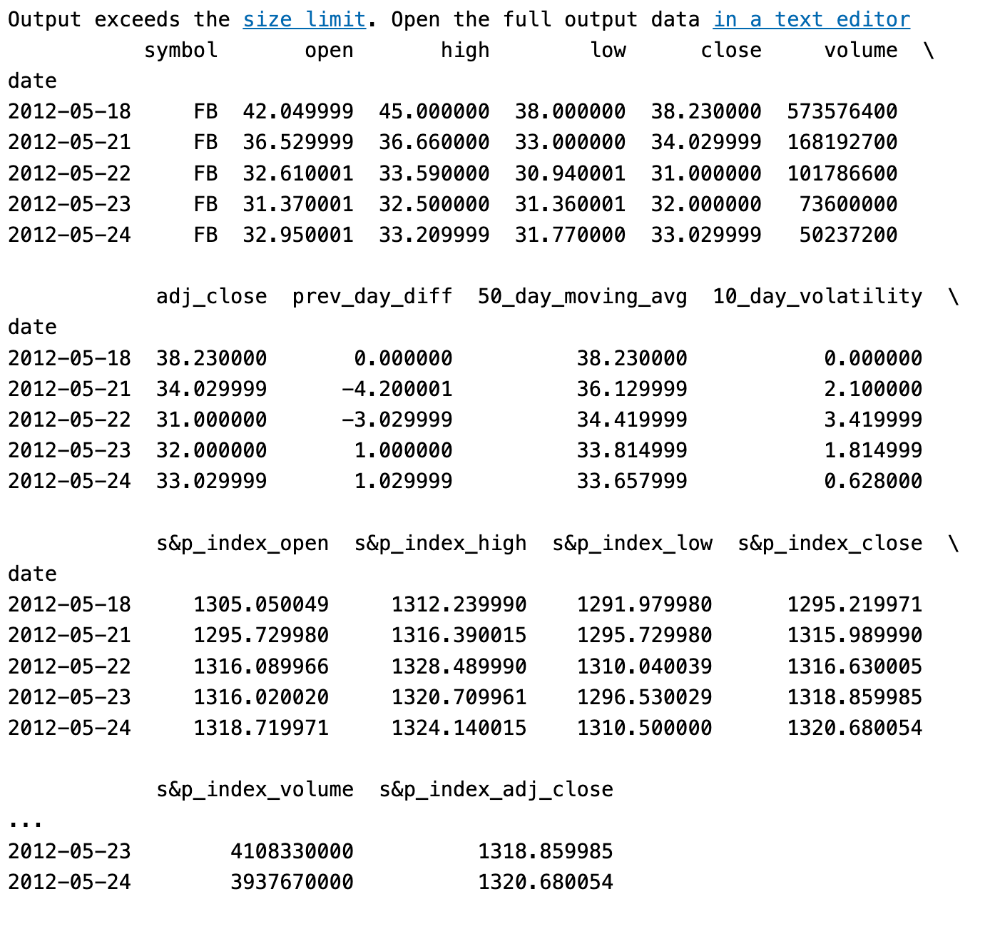
This code defines a lambda function named dateparse that converts a string representing a date into a datetime object using the strptime() function from the datetime module in pandas. A date in the format ‘YYYY-MM-DD’ is represented by the input string ‘%Y-%m-%d’.
It then reads a CSV file named ‘FB.csv’ located at ‘/home/Major_Project/Final-Data/’. The file is read using the pandas function read_csv(). The read_csv() function takes three arguments:
parse_dates=’date’ indicates that the ‘date’ column in the CSV file should be parsed as dates rather than simple strings.
index_col=’date’ specifies that the ‘date’ column should be used as the index of the resulting DataFrame. This means that the DataFrame will be indexed by the dates instead of default numerical indices.
date_parser=dateparse specifies the custom date parsing function to be used. In this case, it uses the dateparse lambda function defined earlier.
Using the head() function, the code prints the first few rows of the resulting DataFrame. The preview includes the column names, the parsed date values as the index, and a subset of the actual data.
#check datatype of index
data.index
In a DataFrame named data, this code checks the data type of the index. DataFrame rows are indexed by their labels or identifiers.
This code retrieves the index object from the DataFrame by calling data.index. Each row in the DataFrame has an index value represented by this object. The purpose of this code is to determine the index’s data type.
As a result of this code, the data type of the index will be displayed. Integers, strings, dates, and timestamps are all data types supported by pandas. A DataFrame’s data type can be used to gain insight into its structure and organization.
#convert to time series:
ts = data['adj_close']
ts.head(10)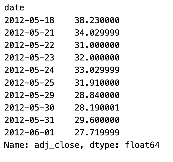
DataFrame column data is converted into a time series object, and the first ten values of the time series are displayed.
Assigning the column with the label ‘adj_close’ to a new variable called ts, the line ts = data[‘adj_close’] selects the column from the DataFrame with the label ‘adj_close’. It is assumed that this column contains data about the adjusted closing prices of a stock or another financial instrument.
To display the first 10 values of the time series, the line ts.head(10) extracts the ‘adj_close’ column and assigns it to ts. Pandas’ head() method returns a number of rows from a Series or DataFrame’s beginning.
This code creates a time series by converting a specific column from a DataFrame. After that, the first 10 values of the time series are shown, giving a glimpse of historical adjusted closing prices.
Indexing TS Array
#1. Specific the index as a string constant:
ts['2012-05-18']
Based on an index value, this code accesses a specific value from a time series object, ts.
Within square brackets, the line ts[‘2012–05–18’] specifies the index value ‘2012–05–18’. It is assumed that this index value represents a date or timestamp.
The purpose of this code is to retrieve the value from the time series ts that corresponds to the specified index value, in this case May 18, 2012.
This code retrieves a specific value from a time series object by specifying the index value as a string constant.
#2. Import the datetime library and use 'datetime' function:
from datetime import datetime
ts[datetime(2015, 3, 26)]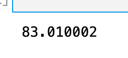
The following code snippet performs the following actions:
A datetime class is imported from the datetime module in the Python standard library. This class provides functionality for manipulating and representing dates and times.
This line creates a datetime object representing March 26, 2015 by utilizing the datetime function. The datetime object is constructed by passing the year, month, and day as arguments.
The purpose of this code is to access a specific value from the time series TS using the datetime object. It retrieves the value in the time series corresponding to the specified date by indexing ts with the datetime object.
A datetime object representing a specific date is created by importing the datetime class, and then a value is retrieved from a time series using this datetime object.
Checking For Stationary
Plot Time Series
plt.plot(ts) 
A line plot of the values in a time series object, ts, is created using the plot() function in the matplotlib.pyplot library.
A graph is generated by plt.plot(ts). On the x-axis are the index values of the time series (e.g., dates or timestamps), and on the y-axis are the values of ts.
Data in the time series will be visualized using this code to reveal trend and patterns. This graph illustrates the changes in values over time.
By displaying the data as a line plot, we can identify any patterns or trends that exist in the series and visualize the data.
Function for testing stationarity
from statsmodels.tsa.stattools import adfuller

def test_stationarity(timeseries):

    #Determing rolling statistics
    rolmean = pd.rolling_mean(timeseries, window=20)
    rolstd = pd.rolling_std(timeseries, window=20)

    #Plot rolling statistics:
    orig = plt.plot(timeseries, color='blue',label='Original')
    mean = plt.plot(rolmean, color='red', label='Rolling Mean')
    std = plt.plot(rolstd, color='black', label = 'Rolling Std')
    plt.legend(loc='best')
    plt.title('Rolling Mean & Standard Deviation')
    plt.show(block=False)

    #Perform Dickey-Fuller test:
    print 'Results of Dickey-Fuller Test:'
    dftest = adfuller(timeseries, autolag='AIC')
    dfoutput = pd.Series(dftest[0:4], index=['open','high','10_day_volatility', '50_day_moving_avg'])
    for key, value in dftest[4].items():
        dfoutput['Critical Value (%s)'%key] = value
    print dfoutput
This code contains a function called test_stationarity that tests a given time series’ stationarity.
Adfuller is assumed to be imported from statsmodels.tsa.stattools.
An analysis of time series data is performed with the test_stationarity function using the timeseries parameter.
The function contains the following:
From the pandas library, rolling statistics are calculated using rolling_mean and rolling_std functions. Window specifies how large the rolling window should be, in this case 20.
The rolling mean (in red) and rolling standard deviation (in black) are visualized in a plot.
A Dickey-Fuller test is performed using the adfuller function. Time series are tested for stationaryness with this test. DFtest stores the test results.
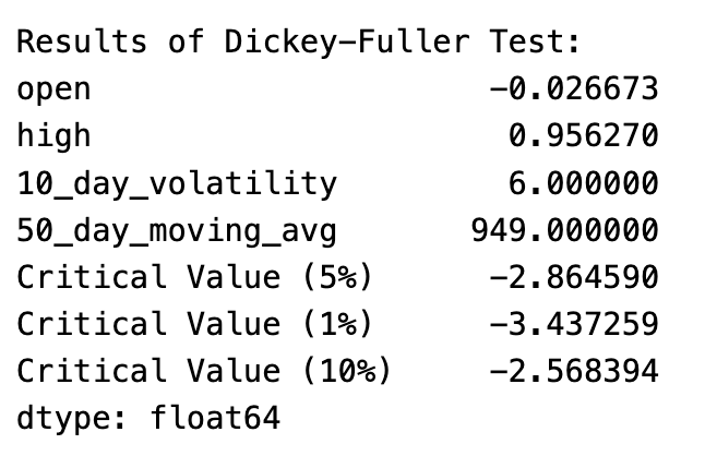
With the print statement, the test results, including test statistics and critical values, are displayed. A test result is stored and formatted using the dfoutput variable.
The code provides a function for calculating rolling statistics and conducting Dickey-Fuller tests to determine whether a time series is stationary. It analyzes the opening price, high price, volatility over 10 days, and moving average over 50 days of the time series.
test_stationarity(ts)
In this code snippet, a time series object, ts, is passed as an argument to the test_stationarity function.
When test_stationarity(ts) is executed, the function defined earlier will be invoked and perform the following steps:
Ts time series are calculated with a window size of 20 to determine the rolling mean and rolling standard deviation.
Show the rolling mean in red, the rolling standard deviation in black, and the original time series in blue.
To visualize rolling standard deviation and rolling mean, show the plot.
Test the stationarity of the ts time series using the Dickey-Fuller test.
Provide a printout of the Dickey-Fuller test results, including test statistics, critical values, and other statistics.
To assess the stationarity of the ts series, call test_stationarity(ts) to apply a series of statistical tests and visualizations.
Estimating & Eliminating Trend
ts_log = np.log(ts)
plt.plot(ts_log)
In this code snippet, the logarithm of the values of a time series, ts, is taken and the resulting transformed series is plotted.
To each value of the ts time series, ts_log = np.log(ts) applies the natural logarithm function from the numpy library (np.log()). A new variable called ts_log is created from the transformed series.
In the next line, plt.plot(ts_log) uses the plot() function from the Matplotlib library to plot the transformed series (ts_log). The logarithmically transformed time series are shown in this plot.
With this code, we are aiming to visualize the changes in the data distribution and any potential trends. Logarithms can stabilize variances or amplify small changes.
It plots the transformed series to observe any patterns or changes in the data that may be apparent after taking the logarithm of a time series and assigning it to a new variable (ts_log).
Smoothing
Moving Average
moving_avg = pd.rolling_mean(ts_log, 10, min_periods=1)
plt.plot(ts_log)
plt.plot(moving_avg, color='red')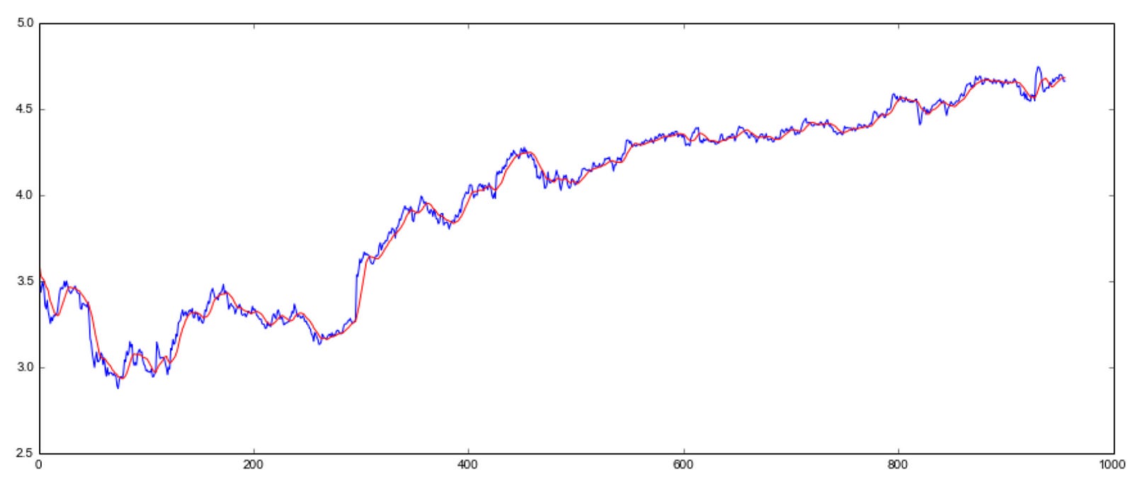
Using this code snippet, the moving average is calculated for a logarithmically transformed time series, ts_log, and the original series is plotted along with the moving average.
Using moving_avg = pd.rolling_mean(ts_log, 10, min_periods=1), the moving average of the ts_log time series can be calculated. With min_periods=1, even if there are fewer than 10 data points, the moving average is still computed with a rolling window of size 10.
Plotting the original logarithmically transformed data series (ts_log) is then created using plt.plot(ts_log).
Plotting the moving average series on the same plot with color ‘red’ follows plt.plot(moving_avg, color=’red’).
The purpose of this code is to visualize the original time series as well as its corresponding moving average. Data trends can be identified and short-term fluctuations can be smoothed out with the moving average.
The code calculates the moving average of a logarithmically transformed time series and plots both the original and moving average to visualize the data and underlying trends.
test_stationarity(ts_log_moving_avg_diff)

To determine stationarity, the code snippet calls the test_stationarity function and compares the logarithmically transformed series with the moving average series, ts_log_moving_avg_diff.
Upon executing test_stationarity(ts_log_moving_avg_diff), the function defined earlier will be invoked and the following steps will be performed:
The rolling mean and rolling standard deviation of the ts_log_moving_avg_diff time series should be calculated.
Put the rolling mean in red, the rolling standard deviation in black, and the original time series (ts_log_moving_avg_diff) in blue.
Visualize the rolling mean and rolling standard deviation of the difference series with the plot.
Test the stationarity of the ts_log_moving_avg_diff time series using the Dickey-Fuller test.
The Dickey-Fuller test results, including the test statistic, critical values, and other statistics, should be printed.
By subtracting the moving average from the logarithmically transformed series, test_stationarity(ts_log_moving_avg_diff) assesses the stationarity of the difference series.