Strategic Portfolio Allocation with Python: A Global Perspective

Using Data from S&P 500, TSX, STOXX 600, and SSE to Build and Optimize Investment Portfolios

Sep 06, 2024

∙ Paid

Source code at the end!

In today’s rapidly evolving financial landscape, the ability to analyze, optimize, and visualize investment strategies has become crucial for making informed decisions. Leveraging Python’s powerful libraries, this article explores an in-depth approach to portfolio optimization using real-world data from Yahoo Finance. By focusing on four major stock indices — the S&P 500, TSX, STOXX 600, and SSE — the analysis demonstrates how various strategies, such as buy-and-hold and maximizing the Sharpe ratio, can enhance returns. Through data manipulation, visualization, and portfolio balancing, Python provides a dynamic framework for financial modeling, enabling investors to diversify risk and optimize their portfolios effectively.

In this guide, you will learn how to retrieve market data, process it, and apply optimization techniques to achieve balanced, risk-adjusted returns. Whether you’re a seasoned investor or new to portfolio management, this article offers practical insights and code implementations to help maximize your investment potential.

# python 3.7

# For yahoo finance
import io
import re
import requests

# The usual suspects
import numpy             as np
import pandas            as pd
import matplotlib.pyplot as plt

#  Fancy graphics
plt.style.use('seaborn')

# Getting Yahoo finance data
def getdata(tickers,start,end,frequency):
    OHLC    = {}
    cookie  = ''
    crumb   = ''
    res     = requests.get('https://finance.yahoo.com/quote/SPY/history')
    cookie  = res.cookies['B']
    pattern = re.compile('.*"CrumbStore":\{"crumb":"(?P<crumb>[^"]+)"\}')
    for line in res.text.splitlines():
        m = pattern.match(line)
        if m is not None:
            crumb = m.groupdict()['crumb']
    for ticker in tickers:
        url_str  = "https://query1.finance.yahoo.com/v7/finance/download/%s"
        url_str += "?period1=%s&period2=%s&interval=%s&events=history&crumb=%s"
        url = url_str % (ticker, start, end, frequency, crumb)
        res = requests.get(url, cookies={'B': cookie}).text
        OHLC[ticker] = pd.read_csv(io.StringIO(res), index_col=0,
                                   error_bad_lines=False).replace('null', np.nan).dropna()
        OHLC[ticker].index = pd.to_datetime(OHLC[ticker].index)
        OHLC[ticker] = OHLC[ticker].apply(pd.to_numeric)
    return OHLC

# Assets under consideration
tickers = ['%5EGSPTSE','%5EGSPC','%5ESTOXX','000001.SS']

# If yahoo data retrieval fails, try until it returns something
data = None
while data is None:
    try:
        data = getdata(tickers,'946685000','1685008000','1d')
    except:
         pass

ICP = pd.DataFrame({'SP500':    data['%5EGSPC']['Adj Close'],
                    'TSX':      data['%5EGSPTSE']['Adj Close'],
                    'STOXX600': data['%5ESTOXX']['Adj Close'],
                    'SSE':      data['000001.SS']['Adj Close']}).fillna(method='ffill')

# since last commit, yahoo finance decided to mess up (more) some of the tickers data, so now we have to drop rows...
ICP = ICP.dropna()

Data for various stock market indexes are retrieved from Yahoo Finance using this Python script. For fetching and manipulating data, it uses a library called requests, and for processing it, it uses a library called pandas.

As the script begins, it imports libraries such as io for handling strings, re for regular expressions, requests for making HTTP requests, and numpy and pandas for analyzing the data. Matplotlib’s plot style can be set to ‘seaborn’ by using this code.

There is a main function, getdata, that takes a list of ticker symbols as well as a start date, an end date, and a frequency to retrieve data from the ticker symbols. The first thing this function does is to send a request to Yahoo Finance so that a cookie and a crumb value can be obtained for authentication purposes. As a result, the application constructs a URL for each ticker containing the appropriate parameters depending on the data range and frequency of the ticker.

We load the response data into a pandas DataFrame, converting ‘null’ strings into NaN values, and removing rows without any data at the end of the dataframe. In order to convert the date index to a datetime format, it must be converted to a datetime format.

After identifying a list of tickers for various indices, the script attempts to fetch data using the getdata function repeatedly until success is achieved by retrieving the data for each ticker. Thereafter, once the data has been retrieved, the DataFrame named ICP is created by consolidating all the adjusted closing prices into one DataFrame, filling in any missing values with the previous data points, and removing any remaining rows with NaN values.

BuyHold_SP     = ICP['SP500']    /float(ICP['SP500'][:1])   -1
BuyHold_TSX    = ICP['TSX']      /float(ICP['TSX'][:1])     -1
BuyHold_STOXX  = ICP['STOXX600'] /float(ICP['STOXX600'][:1])-1
BuyHold_SSE    = ICP['SSE']      /float(ICP['SSE'][:1])     -1

BuyHold_25Each = BuyHold_SP*(1/4) + BuyHold_TSX*(1/4) + BuyHold_STOXX*(1/4) + BuyHold_SSE*(1/4)

There are four stock market indices that this code calculates the return on for a buy and hold investment: the S&P 500, TSX, STOXX 600, and SSE. As part of this calculation, the current value of each index is retrieved from the ICP DataFrame and divided by the initial value to determine the percent change in value since the start of the recording. There is a code in the file that calculates an average return over the four indices, each of which is equally weighted at 25%, after determining the buy and hold return for each index. In this way, a diversified investment strategy in these markets will be measured by a single metric that represents the overall performance of the strategy as a whole.

plt.figure(figsize=(16,6))
plt.plot(BuyHold_SP*100,     label='Buy & Hold USA')
plt.plot(BuyHold_TSX*100,    label='Buy & Hold Canada')
plt.plot(BuyHold_STOXX*100,  label='Buy & Hold Europe')
plt.plot(BuyHold_SSE*100,    label='Buy & Hold China')
plt.plot(BuyHold_25Each*100, label='Buy & Hold 25% Each')
plt.xlabel('Time')
plt.ylabel('Cumulative Return (in %)')
plt.margins(x=0.005,y=0.02)
plt.axhline(y=0, xmin=0, xmax=1, linestyle='--', color='k')
plt.legend()
plt.show()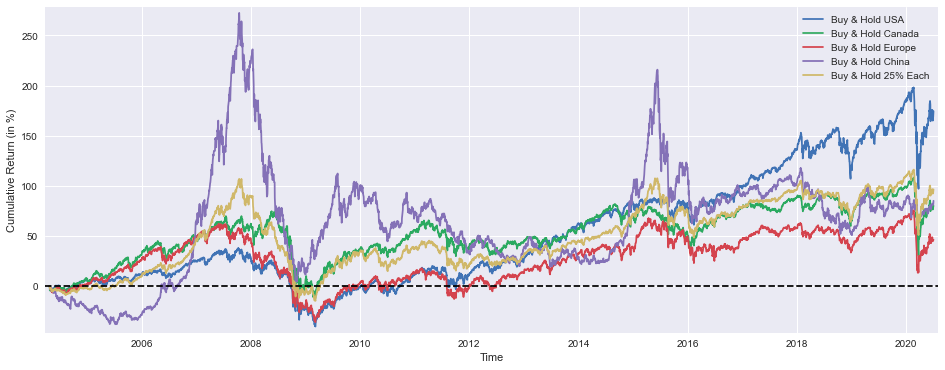

A line plot is generated by this code in order to visualize the cumulative returns of various investment strategies over the course of time. There is a feature built into the system that creates a 16 by 6 inch figure that plots multiple lines for different portfolios, including Buy and Hold strategies for the USA, Canada, Europe, and China, as well as a diversified portfolio with 25% in each region. It is necessary to multiply a return value by 100 in order to present it as a percentage. As you can see from the chart, the x-axis is labeled for time, and the y-axis indicates cumulative returns as a percentage. There is a horizontal reference line at zero included in the plot so that it can be used for performance evaluation and margins are defined to keep data points off the plot edges. Using plt.show(), the figure will be displayed which identifies the different strategies, and a legend will identify them.

SP1Y     = ICP['SP500']    /ICP['SP500'].shift(252)   -1
TSX1Y    = ICP['TSX']      /ICP['TSX'].shift(252)     -1
STOXX1Y  = ICP['STOXX600'] /ICP['STOXX600'].shift(252)-1
SSE1Y    = ICP['SSE']      /ICP['SSE'].shift(252)     -1

Each251Y = SP1Y*(1/4) + TSX1Y*(1/4) +STOXX1Y*(1/4) + SSE1Y*(1/4)

As shown in this code snippet, the annual returns are calculated for four different stock indices: the S&P 500, the TSX, the STOXX 600, and the SSE. By dividing the current value of an index by the value from 252 trading days ago and then subtracting 1, the percentage change for each index is calculated. SP1Y, TSX1Y, STOXX1Y, and SSE1Y are the variables used to store the results of this experiment. By averaging the individual returns for the four indices over the specified period of time, the code then uses these individual returns to calculate a variable called Each251Y that represents the average return per year for the four indices over the specified period.

plt.figure(figsize=(16,6))
plt.plot(SP1Y*100,     label='Rolling 1 Year Buy & Hold Return USA')
plt.plot(TSX1Y*100,    label='  ""  ""  Canada')
plt.plot(STOXX1Y*100,  label='  ""  ""  Europe')
plt.plot(SSE1Y*100,    label='  ""  ""  China')
plt.plot(Each251Y*100, label='  ""  ""  25% Each')
plt.xlabel('Time')
plt.ylabel('Returns (in %)')
plt.margins(x=0.005,y=0.02)
plt.axhline(y=0, xmin=0, xmax=1, linestyle='--', color='k')
plt.legend()
plt.show()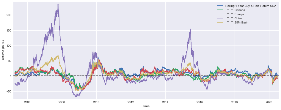

Using Matplotlib, the following code creates a line plot that visualizes financial return data over time for various markets using a line plot using Matplotlib. Using a figure size of 16 by 6 inches, we are able to present multiple datasets clearly on the same page as a single figure. As a result of each call to plt.plot(), investors will be able to see the returns over the past one year of the USA, Canada, Europe, and China, and a combined dataset from each region with equal weight will also be shown. A percentage chart is presented on the y-axis of the chart based on the returns multiplied by 100.

The x-axis of the graph is labeled Time, while the y-axis is labeled Returns in percent, which are both measured in years. This function adds padding to the plot so that data points do not get pushed to the edges due to the padding added by plt.margins(). The horizontal dashed line at y=0 indicates that there is no return to zero. Each dataset is accompanied by a legend which helps the reader identify which line corresponds to which dataset on the graph. After this, plt.show() renders the plot so that it can be viewed.

marr      = 0 #minimal acceptable rate of return (usually equal to the risk free rate)
SP1YS     = (SP1Y.mean()    -marr) /SP1Y.std()
TSX1YS    = (TSX1Y.mean()   -marr) /TSX1Y.std()
STOXX1YS  = (STOXX1Y.mean() -marr) /STOXX1Y.std()
SSE1YS    = (SSE1Y.mean()   -marr) /SSE1Y.std()
Each251YS = (Each251Y.mean()-marr) /Each251Y.std()

print('SP500 1 Year Buy & Hold Sharpe Ratio =',round(SP1YS,2))
print('TSX      "" "" =',round(TSX1YS   ,2))
print('STOXX600 "" "" =',round(STOXX1YS ,2))
print('SSE      "" "" =',round(SSE1YS   ,2))
print('25% Each "" "" =',round(Each251YS,2))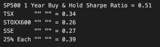

With the help of this code, we can calculate and print the Sharpe Ratio over a period of a year for various financial indices. By adjusting for risk for each investment, the Sharpe Ratio determines the excess return relative to the volatility of an investment when compared to a risk-free investment, indicating the excess return relative to a risk-free investment. It is set to zero by default, which represents a minimal acceptable rate of return, with marr being set to zero. Taking the mean return for each index, including S&P 500, TSX, STOXX 600, SSE, and a composite index, the code calculates the Sharpe Ratio by subtracting marr from the mean return and dividing by the standard deviation of the return. The results, which have been rounded to two decimal places, are printed alongside messages identifying each index and their values.

from scipy.optimize import minimize

def multi(x):
    a, b, c, d = x
    return a, b, c, d   #the "optimal" weights we wish to discover

def maximize_sharpe(x): #objective function
    weights = (SP1Y*multi(x)[0] + TSX1Y*multi(x)[1]
               + STOXX1Y*multi(x)[2] + SSE1Y*multi(x)[3])
    return -(weights.mean()/weights.std())

def constraint(x):      #since we're not using leverage nor short positions
    return 1 - (multi(x)[0]+multi(x)[1]+multi(x)[2]+multi(x)[3])

cons = ({'type':'ineq','fun':constraint})
bnds = ((0,1),(0,1),(0,1),(0,1))
initial_guess = (1, 0, 0, 0)

# this algorithm (SLSQP) easly gets stuck on a local
# optimal solution, genetic algorithms usually yield better results
# so my inital guess is close to the global optimal solution

ms = minimize(maximize_sharpe, initial_guess, method='SLSQP',
              bounds=bnds, constraints=cons, options={'maxiter': 10000})

msBuyHoldAll = (BuyHold_SP*ms.x[0] + BuyHold_TSX*ms.x[1]
                + BuyHold_STOXX*ms.x[2] + BuyHold_SSE*ms.x[3])

msBuyHold1yAll = (SP1Y*ms.x[0] + TSX1Y*ms.x[1]
                   + STOXX1Y*ms.x[2] + SSE1Y*ms.x[3])

It is a Python code which utilizes the SciPy library for optimizing portfolios with four assets with the purpose of maximising their Sharpe ratio. It is possible to return the weights of these assets using the multi function, which takes a vector x as an input and returns it as a result. It is important to note that the maximize_sharpe function serves as the optimization objective in that it calculates the portfolio’s weighted returns based on the asset returns and weights from multi, therefore returning the negative of the Sharpe ratio in contrast to the minimize function which reduces values.

In the optimization process, the constraint function ensures that the weights sum to 1 in order to adhere to the principles of no leverage and no short-selling, and this constraint function is included in the optimization process. In order to initiate the optimization process, weights are put into a range between 0 and 1, defined by a variable called bnds, with a first guess used as an initial guess.

Using the Sequential Least Squares Programming method, the minimize function determined the optimal weights for maximizing the Sharpe ratio within the specified constraints and bounds by utilizing the Sequential Least Squares Programming method! A second calculation is performed to determine the portfolio values for a buy-and-hold strategy, as well as a one-year return mix using the optimized weights, and the results are stored in two variables, msBuyHoldAll and msBuyHold1yAll, respectively.

plt.figure(figsize=(16,6))
plt.plot(BuyHold_SP*100,     label='Buy & Hold S&P500')
plt.plot(BuyHold_25Each*100, label='  ""  ""  25% of Each')
plt.plot(msBuyHoldAll*100,   label='  ""  ""  Max Sharpe')
plt.xlabel('Time')
plt.ylabel('Cumulative Return (in %)')
plt.margins(x=0.005,y=0.02)
plt.axhline(y=0, xmin=0, xmax=1, linestyle='--', color='k')
plt.legend()
plt.show()

print('SP500 Weight =',round(ms.x[0]*100,2),'%')
print('TSX ""       =',round(ms.x[1]*100,2),'%')
print('STOXX600 ""  =',round(ms.x[2]*100,2),'%')
print('SSE ""       =',round(ms.x[3]*100,2),'%')
print()
print('Sharpe =',round(msBuyHold1yAll.mean()/msBuyHold1yAll.std(),3))
print()
print('Median yearly excess return over SP500 =',round((msBuyHold1yAll.median()-SP1Y.median())*100,1),'%')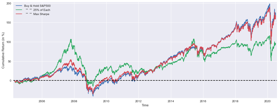

As a result of this code, a plot can be created that shows the cumulative returns on various investment strategies compared with S&P 500 performance. With this tool, you are able to generate a 16 x 6 inch figure and plot three strategies as percentages on it. A number of the strategies used by these funds are Buy and Hold strategies for the S&P 500, diversified portfolios that place equal weights on four assets, and Max Sharpe strategies designed to maximize risk-adjusted returns based on risk-adjusted returns. On the plot, we have defined margins for the x and y axes to define the axes for the time and cumulative returns percentage, as well as the axes for the time. The horizontal dashed line at zero y coordinate serves as a reference, and a legend is displayed before each figure to highlight the strategy that is being used.

When the plot has been completed, the code will output numerical results, including the weights of the four assets in the Max Sharpe portfolio in percentages, the Sharpe Ratio calculated from the average and standard deviations of one-year returns, as well as the median excess return over the S&P 500 for the year. There are two key quantitative insights and a visual representation of the investment strategies’ performance, which is effectively summarized throughout the report.

def maximize_median_yearly_return(x): #different objective function
    weights = (SP1Y*multi(x)[0] + TSX1Y*multi(x)[1]
               + STOXX1Y*multi(x)[2] + SSE1Y*multi(x)[3])
    return -(float(weights.median()))

mm = minimize(maximize_median_yearly_return, initial_guess, method='SLSQP',
              bounds=bnds, constraints=cons, options={'maxiter': 10000})

mmBuyHoldAll = (BuyHold_SP*mm.x[0] + BuyHold_TSX*mm.x[1]
                + BuyHold_STOXX*mm.x[2] + BuyHold_SSE*mm.x[3])

mmBuyHold1yAll = (SP1Y*mm.x[0] + TSX1Y*mm.x[1]
                   + STOXX1Y*mm.x[2] + SSE1Y*mm.x[3])

By using the function maximize_median_yearly_return, we can optimize the weights of our portfolio so that its median yearly return is maximized across four stock indices: SP, TSX, STOXX, and SSE. In this program, the combined weighted return is calculated by using a given set of weights and influencing them with one or more input variables. The median of these returns is returned as a negative value to accommodate the minimize function, thereby maximizing the median return by allowing the function to negate itself.

Using maximize_median_yearly_return from an optimization library, the code uses the minimize function to determine the optimal weights for the portfolio by utilizing a function called minimize in order to determine the optimal weights to use. It begins with an initial guess and uses the Sequential Least Squares Programming method to optimize the weights according to set bounds and constraints, with a maximum of 10,000 iterations allowed for the optimization process before the solution is found.

As soon as the code has obtained the optimal weights for every stock index, it calculates two portfolio returns: mmBuyHoldAll, which represents a buy-and-hold strategy with the optimized weights for each stock index, and mmBuyHold1yAll, which represents the weighted yearly return for the same stock index for the same year. Compared to a static Buy-and-Hold portfolio, this shows the potential performance of the optimized portfolio when compared to the performance of the static portfolio.

plt.figure(figsize=(16,6))
plt.plot(BuyHold_SP*100,     label='Buy & Hold S&P500')
plt.plot(BuyHold_25Each*100, label='  ""  ""  25% of Each')
plt.plot(mmBuyHoldAll*100,   label='  ""  ""  Max 1Y Median')
plt.xlabel('Time')
plt.ylabel('Cumulative Return (in %)')
plt.margins(x=0.005,y=0.02)
plt.axhline(y=0, xmin=0, xmax=1, linestyle='--', color='k')
plt.legend()
plt.show()

print('SP500 Weight =',round(mm.x[0]*100,2),'%')
print('TSX ""       =',round(mm.x[1]*100,2),'%')
print('STOXX600 ""  =',round(mm.x[2]*100,2),'%')
print('SSE ""       =',round(mm.x[3]*100,2),'%')
print()
print('Sharpe =',round(mmBuyHold1yAll.mean()/mmBuyHold1yAll.std(),3))
print()
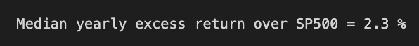
print('Median yearly excess return over SP500 =',round((mmBuyHold1yAll.median()-SP1Y.median())*100,1),'%')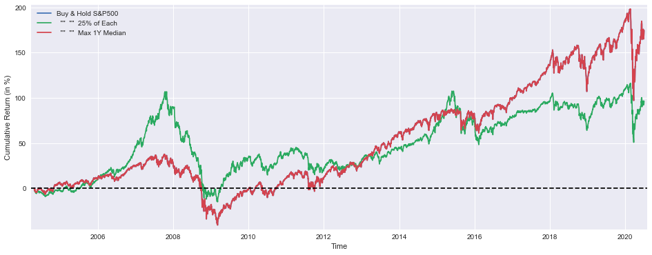

This code creates a plot that allows the user to visualize the cumulative returns of various investment strategies over the course of time compared to the S&P 500 index. The tool creates a figure of a given size and plots three strategies, namely the Buy and Hold strategy for the S&P 500, the portfolio strategy with an equal allocation of assets across the portfolio, and the maximum one-year median return strategy. Time is shown as the x-axis, while Cumulative Return in percentage is shown on the y-axis, which provides context for the data by providing a sense of time. For clarity purposes, the plot includes margins at the top and bottom to differentiate positive and negative returns, as well as a horizontal dashed line to represent the zero point. Each strategy is indicated by a legend at the bottom of the chart.

A few lines after the plot is created by the code, the weights calculated for the portfolio assets are printed in two decimal places as well. The Sharpe ratio is also computed and displayed, which shows the risk-adjusted return of the various strategies based on their risk-adjusted performance. Last but not least, it calculates and prints the median yearly excess return of the strategies in comparison with the S&P 500, which provides an insight into their performance relative to this benchmark.

YTD_SP     = ICP['SP500'][-252:]    /float(ICP['SP500'][-252])   -1
YTD_TSX    = ICP['TSX'][-252:]      /float(ICP['TSX'][-252])     -1
YTD_STOXX  = ICP['STOXX600'][-252:] /float(ICP['STOXX600'][-252])-1
YTD_SSE    = ICP['SSE'][-252:]      /float(ICP['SSE'][-252])     -1

YTD_25Each = YTD_SP*(1/4) + YTD_TSX*(1/4) + YTD_STOXX*(1/4) + YTD_SSE*(1/4)

YTD_max_sharpe = YTD_SP*ms.x[0] + YTD_TSX*ms.x[1] + YTD_STOXX*ms.x[2] + YTD_SSE*ms.x[3]
YTD_max_median = YTD_SP*mm.x[0] + YTD_TSX*mm.x[1] + YTD_STOXX*mm.x[2] + YTD_SSE*mm.x[3]

It consists of a function that extracts the last 252 data points from each of the respective indexes in order to compute the return relative to the value at the start of this period for the S&P 500, TSX, STOXX 600, and SSE indices. The return of the investment can be calculated by dividing the current value by the starting value minus one. This type of data is then averaged with equal weights assigned to each index, resulting in a value that is stored in YTD_25Each as a result of the average. In addition, the code also calculates two YTD returns by using different weighting schemes represented by the variables ms.x and mm.x, which likely correspond to weights that are optimized for maximum Sharpe ratios and maximum median returns as well. We store the YTD_max_sharpe and YTD_max_median results in YTD_max_sharpe and YTD_max_median, respectively.

plt.figure(figsize=(15,6))
plt.plot(YTD_SP*100,         label='YTD Buy & Hold S&P500')
plt.plot(YTD_25Each*100,     label='  ""  ""  25% of Each')
plt.plot(YTD_max_sharpe*100, label='  ""  ""  Max Sharpe')
plt.plot(YTD_max_median*100, label='  ""  ""  Max 1Y Median')
plt.xlabel('Time')
plt.ylabel('Cumulative Return (in %)')
plt.margins(x=0.005,y=0.02)
plt.axhline(y=0, xmin=0, xmax=1, linestyle='--', color='k')
plt.legend()
plt.show()

print('Buy & Hold S&P500 YTD Performance (at 1 July 2020) =',round(float(YTD_SP[-1:]*100),1),'%')
print(' "" "" 25% of Each   "" "" =',round(float(YTD_25Each[-1:]*100),1),'%')
print(' "" "" Max Sharpe    "" "" =',round(float(YTD_max_sharpe[-1:]*100),1),'%')
print(' "" "" Max 1Y Median "" "" =',round(float(YTD_max_median[-1:]*100),1),'%')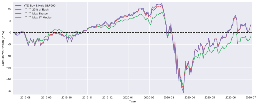

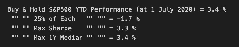
This code allows you to generate a visual representation of cumulative returns for various investment strategies over a specified period of time compared to the S&P 500. It uses Matplotlib to create a line plot that illustrates Year-To-Date performance as a percentage for each strategy, based on the performance as it is represented by the different lines in the plot. Depending on the investment strategy, the size of the plot can be changed from 15 by 6 inches to a percentage format, which is based on the YTD values of each strategy. There is a name for each line that corresponds to the corresponding strategy on the graph. This chart shows the cumulative return in percentages on the x-axis, and the time on the y-axis is labeled Time. In order to enhance the appearance of the plot, the margins have been increased, and the dashed line at y equals zero indicates break-even performance. Moreover, the plot is displayed at the end of the command, and a legend is included. There is also a summary of the performance of each strategy below the plot, displaying the YTD returns formatted with one decimal place for quick reference, as well as the performance summary for each strategy.

ICP['SPRet']    = ICP['SP500'] /ICP['SP500'].shift(1)-1
ICP['SSERet']   = ICP['SSE']   /ICP['SSE'].shift(1)  -1

ICP['Strat'] = ICP['SPRet'] * 0.8 + ICP['SSERet'] * 0.2

ICP['Strat'][SP1Y.shift(1)  > -0.17] = ICP['SSERet']*0 + ICP['SPRet']*1
ICP['Strat'][SSE1Y.shift(1) > 0.29]  = ICP['SSERet']*1 + ICP['SPRet']*0

DynAssAll    = ICP['Strat'].cumsum()
DynAssAll1y  = ICP['Strat'].rolling(window=252).sum()
DynAssAllytd = ICP['Strat'][-252:].cumsum()

This code performs financial calculations on a DataFrame called ICP, which contains values for the S&P 500 index and the SSE index on a daily basis. Whenever the current day’s value is divided by the previous day’s value, the daily returns for both indices are calculated by subtracting one for each index from the current day’s value. It is based on the assumption that the S&P 500 will return 80% of the returns while the SSE will return 20%, with the strategy being defined as a weighted combination of these returns. It is important to note that the strategy is adjusted based on specific conditions, such as the following: if the one-year shift of the S&P 500 return exceeds -0.17, the strategy will fully invest in the S&P 500, while if the one-year shift of the SSE return exceeds 0.29, the strategy will fully invest in the SSE. A final calculation is carried out in the code in order to get the cumulative sum of the strategy return over time, which is then stored in DynAssAll. The DynAssAll1y algorithm also computes a rolling sum of the strategy over a time period of one year, whereas the DynAssAllytd algorithm captures the cumulative sum of the strategy for the past 252 days, which is the latest year.

plt.figure(figsize=(15,6))
plt.plot(BuyHold_SP*100,     label='Buy & Hold SP&500')
plt.plot(mmBuyHoldAll*100,   label='  ""  ""  Max 1Y Median')
plt.plot(DynAssAll*100,      label='Dynamic Asset Allocation')
plt.xlabel('Time')
plt.ylabel('Cumulative Return (in %)')
plt.margins(x=0.005,y=0.02)
plt.axhline(y=0, xmin=0, xmax=1, linestyle='--', color='k')
plt.legend()
plt.show()

print('Median yearly excess return over SP500 =',round(float(DynAssAll1y.median()-SP1Y.median())*100,1),'%')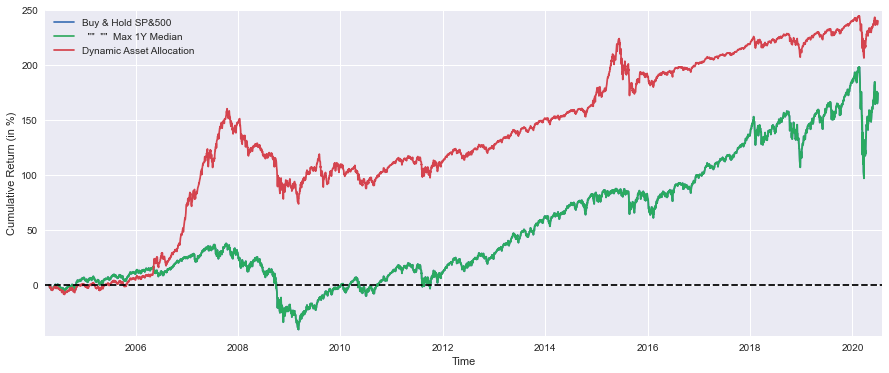

Matplotlib provides a convenient tool for creating visual comparisons between various investment strategies via this code snippet. An area of 15 by 6 inches is set up and three time series representing cumulative returns are plotted: a Buy and Hold strategy based on the S&P 500, a Maximum 1-year Median Return strategy, and a Dynamic Asset Allocation strategy. In order to represent percentages, the values are multiplied by 100, and each line is appropriately labeled to show the percentage. X-axis is labeled Time, and Y-axis is labeled Cumulative Return in %, which improves the clarity of the figure. The plot includes an indication of the break-even point at y=0, as well as a horizontal dashed line at y=0 to indicate the break-even point, as well as a legend for the lines so they can be identified easily. As you can see, the graph is displayed using the plt.show() function.

As a result of plotting, the code computes the median annual excess return of the Dynamic Asset Allocation strategy relative to the S&P 500. The result is rounded to one decimal place and expressed in percentage form, providing further insight into the performance of the analyzed strategies.

plt.figure(figsize=(15,6))
plt.plot(YTD_SP*100,         label='YTD Buy & Hold S&P500')
plt.plot(YTD_max_median*100, label='  ""  ""  Max 1Y Median')
plt.plot(DynAssAllytd*100,   label='Dynamic Asset Allocation')
plt.xlabel('Time')
plt.ylabel('Cumulative Return (in %)')
plt.margins(x=0.005,y=0.02)
plt.axhline(y=0, xmin=0, xmax=1, linestyle='--', color='k')
plt.legend()
plt.show()

print('Buy & Hold S&P500 YTD Performance (at 1 July 2020) =',round(float(YTD_SP[-1:]*100),1),'%')
print(' "" "" Max 1Y Median "" ""  =',round(float(YTD_max_median[-1:]*100),1),'%')
print(' Strategy YTD Performance   =',round(float(DynAssAllytd[-1:]*100),1),'%')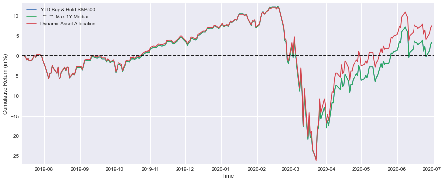

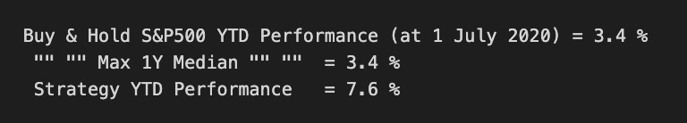
Using Matplotlib, this code snippet displays the year-to-date performance of three investment strategies based on the S&P 500 index: a Buy and Hold strategy based on the index, a maximum 1-year median performance strategy, and a Dynamic Asset Allocation strategy based on the index. In this plot, the dimensions are set to 15 inches wide by 6 inches tall, and for the sake of clarity, each strategy’s cumulative return is depicted as a percentage instead of a number. Time is represented on the X-axis, and the Cumulative Return in percentage is displayed on the Y-axis. It has been adjusted to create a better presentation of the margins, and a horizontal dashed line at 0% makes it easier to compare the strategies. It is possible to identify each line on the graph by looking at the legend. As a final step of the code, performance metrics for each strategy as of July 1, 2020, as well as their year-to-date performance, are also printed to the console. This provides an easy means of comparing their performance without requiring the visual interpretation of the plot.

Continue reading this post for free, courtesy of Onepagecode.

Or purchase a paid subscription.