Text Classification: Complete Guide
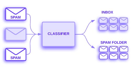
There are a variety of software systems that process text data at scale using text classification algorithms. A program that analyzes emails determines if they should be delivered to the inbox or filt
Topic classification is the process of categorizing a text document into one of a set of predefined categories. Most topic classification problems rely heavily on keywords in the text for categorization.
Don’t live at the mercy of medium paywall. Check the link below and get rid of paywall so you can siphon everything avaialble on substack.
Topic classification is used to flag incoming spam emails, which are filtered into a spam folder.
The sentiment analysis of text content is another type of text classification which aims to identify the type of opinion expressed in the text content: the polarity of this opinion. There are several ways to rate a program. This can be done in the form of a binary like/dislike rating, or in a more granular way, such as a star rating from 1 to 5. There are many examples of sentiment analysis that can be applied to a variety of different situations, including analyzing Twitter posts to discover if the Black Panther movie was liked by the people, as well as predicting whether the general public will like a new brand of Nike shoes based on Walmart reviews.
It will provide you with an overview of some key machine learning best practices that can be used to solve text classification problems. What you will learn from this course is as follows:
Text classification workflow using machine learning, from start to finish
Text classification models: choosing the right one
A step-by-step guide to implementing your TensorFlow model
Workflow for classifying texts
To explain machine learning workflows, here is a high-level overview:
Step 1: Gather Data
Step 2: Explore Your Data
Step 3: Choose a Model*
Step 4: Prepare Your Data
Step 5: Build, Train, and Evaluate Your Model
Step 6: Tune Hyperparameters
Step 7: Deploy Your Model
Step 1: Gather Data
Whenever there is a supervised machine learning problem to solve, gathering data is the first and most significant step. You can only build a text classifier that is as good as the dataset you choose to train it on.
The open-source datasets available can be helpful if you are not trying to solve a specific problem. Instead, you simply want to explore text classification as a whole. There is a variety of them available. Some of them can be found in our GitHub repository, which provides links to some of them. On the other hand, if you are taking on a specific problem, you will need to collect the data necessary to solve it. It is likely that you will be able to leverage one or more of the public APIs provided by the organizations you are trying to work with. This is the Twitter API or the NY Times API, to assist in solving the problem you are attempting to resolve.
When collecting data, it is important to remember the following things:
You should make sure you understand the limitations of the API you intend to use before you use it if you are using a public API. As an example, some APIs limit the number of queries that can be made by you at a given time, for example.
I believe the more examples that you have for training (referred to as samples from now on in this guide), the more effective it will be. By doing this, you will be able to generalize your model more effectively.
Ensure there are not too many or too few samples for every class or topic in order to avoid an imbalance in the number of samples. There should be a similar number of samples in each class, which means you should have a comparable number of samples.
Don’t just sample the common cases; ensure you cover the entire space of possible inputs.
The workflow in this guide will be illustrated by using the movie reviews dataset from the Internet Movie Database (IMDb) so that you can get a feel for the process. In this dataset, you will find movie review columns posted by IMDb users, along with the labels indicating whether the reviewer liked the film or not. The labels indicate if the reviewer had a positive or negative outlook on the movie. In this case, we have a classic example of the application of sentiment analysis.
Step 2: Explore Your Data
The workflow does not end with building and training a model. A better model will be able to be built if you understand the characteristics of your data beforehand. Increasing accuracy could simply mean getting better results. Also, fewer data would be needed for training, or fewer computing resources would be required.
Dataset loading
Let’s start by loading the dataset into Python.
Check the Data
I suggest that after loading the data, you should run a few manual checks to see if it is consistent with your expectations: select a few samples and check if they are consistent with your expectations. If you print a few random samples, for example, you can check whether the sentiment label reflects the sentiment of the review by printing out random samples. As an example of what we mean, let’s look at one review from the IMDb dataset that we chose at random: “Ten minutes of story stretched into the better part of two hours. After the halfway point, there had been nothing of any significance that had occurred, so I should have left.” In this case, the common sentiment (negative) matches the label on the sample.
Collect Key Metrics
In order to gain a clearer understanding of your text classification problem, you should gather the following important metrics once you have verified the data:
There are a total of thousands of examples in your data set, which is called the number of samples.
There are a total number of classes in the data which are categorized as topics or categories.
A class is defined as the number of samples that are included in that class (topic/category). The number of samples in each class will be similar in a balanced dataset, whereas, in an imbalanced dataset, the number of samples in each class will vary considerably.
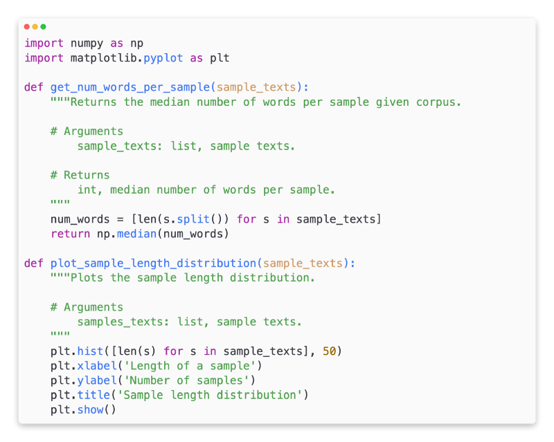
A sample contains a median number of words.
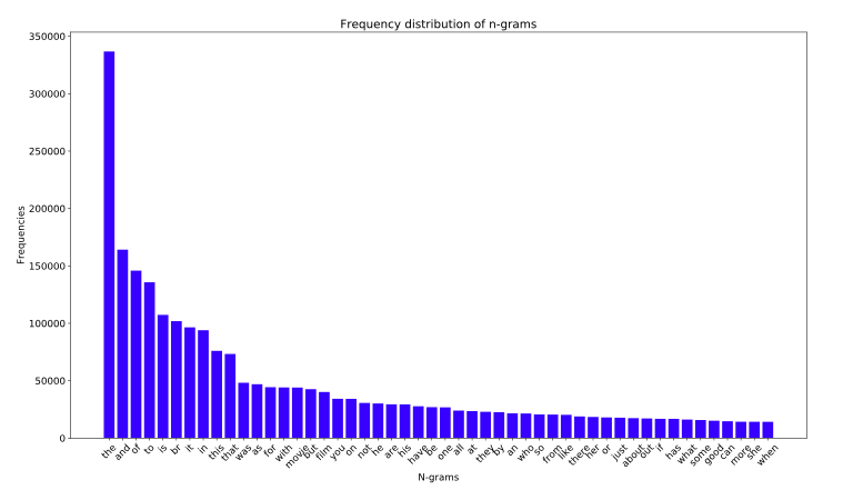
Distribution of words’ frequency (number of occurrences): Average frequency (number of occurrences) of words.
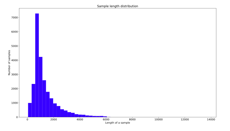
The number of words per sample in the dataset is distributed according to the sample length.
The word-frequency and sample-length distributions for the IMDb reviews dataset are shown in Figures 3 and 4.
These metrics can be calculated and analyzed using explore_data.py. Examples include:
Step 3: Choose A Model
It is at this point in the process that we have assembled our dataset, analyzed it, and gained an insight into its main characteristics. After gathering the metrics we need for Step 2, we will need to decide what classification model we should use based on the metrics we gathered in Step 2. It is necessary to ask questions such as, ‘How do we present the text data in order to be accepted by a program that expects numeric input’? (this is called data preprocessing and vectorization), What type of model should we use?, What configuration parameters should we use for our model?, etc.
Data preprocessing and model configuration options have been developed over decades of research. There is, however, a downside to having access to such a wide array of viable options to choose from since this greatly increases both the complexity and the scope of the specific problem at hand that needs to be solved. As there may not be obvious solutions, a naive approach would be to exhaustly try every possible alternative, while pruning some of the choices based on intuition, since the best options might not be obvious. Nevertheless, that would be a very expensive endeavor.
It is our intention to simplify the process of selecting a text classification model in this guide in an attempt to make it easier for everyone to use. Our goal is to find the algorithm that will achieve close to maximum accuracy on a given dataset while minimizing the computation time required to train it based on the dataset. In this study, we performed 450K experiments across 12 datasets, using different data preprocessing techniques and different model architectures for each dataset, across problems of various types (especially sentiment analysis and topic classification problems). Identifying these parameters helped us identify optimal choices for datasets.
An overview of our experimentation is provided in the model selection algorithm and flowchart below. In the following sections of this guide, we will explain all the terms used in them in detail, so don’t worry if you don’t understand them yet.
Algorithm For Data Preparation And Model Building
The flowchart shows yellow boxes that indicate the processes involved in preparing data and models for analysis. Each process was represented by a grey box and a green box, which indicate the choices that were considered. Our recommendation for each process is indicated in green boxes.
You can use this flowchart as a starting point for constructing your own experiment since it gives you a high level of accuracy at a relatively low computing cost for your first experiment. Over the subsequent iterations, you can continue to improve on your initial model in order to make it more accurate.
There are two key questions that can be answered by this flowchart:
Would it be better to use a learning algorithm or model or both?
In order to effectively learn the relationship between text and label, we need to prepare the data in the appropriate way.
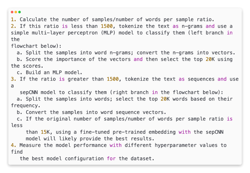
In order to answer the second question, we need to know the answer to the first one. It will be important to determine what model we choose to use in order to preprocess data so it can be fed into the model. Generally speaking, there are two types of word order models: those that use information about the order of words in the text (sequence models) and those that see the text only as a collection of words (n-gram models). In addition to convolutional neural networks (CNNs), recurrent neural networks (RNNs), and their variations, there are also other types of sequence models available. One type of n-gram model is logistic regression, a type of multilayer perceptron that consists of several layers, is also known as a fully-connected neural network, a type of gradient boosted tree and a type of support vector machine.
We have found that the ratio of the number of samples (S) to the number of words per sample (W) correlates with the performance of the model based on the number of samples (S) compared to the number of words per sample (W).
Depending on how small the value of this ratio (*1500) is, small multilayer perceptrons adaptable to n-gram inputs (which we’ll call Option A) will perform better or at least as well as sequence models if the value of the ratio is small. Compared to sequence models, MLP’s are easier to define and understand, and they take a much shorter amount of time to compute than sequence models. The sequence model (Option B) should be used whenever there is a large value for this ratio (greater than 1500). According to the samples/words-per-sample ratio you chose, you can skip ahead to the relevant subsections (labeled A or B) for the model type that you chose based on the steps in the steps that follow.
For the IMDb review dataset we used, the ratio of samples to words-per-sample was *144 in the case of our IMDb review dataset. As a result, we will be creating a model that is based on the MLP algorithm.
Step 4: Prepare Your Data
It is necessary that we transform our data into a format that is understandable by a model before it can be fed into it.
To begin with, it is possible that the samples of data that we have gathered are arranged in a particular order. In order for the relationship between texts and labels to be as strong as possible, any information related to the order of samples should not be used to influence the relationship. A dataset sorted by class and then divided into training/validation sets will not represent the overall data distribution if, for example, the training/validation sets are sorted by class and then divided into training/validation sets.
To ensure that data order is not affecting the model, a simple rule of thumb is to always shuffle the data before doing anything else to ensure that the model is not affected by data order. In case your data is already split into training and validation sets, make sure that as you transform your training data, you also transform your validation data in the same way that you transformed your training data. You can split the samples after shuffling if you do not already have separate training and validation sets, and it is typical to use 80% of the samples for training and 20% for validation, if you do not already have them.
It is also important to keep in mind that machine learning algorithms take numbers as inputs. It is therefore necessary to convert the text into numerical vectors in order to be able to process them. This process has two steps that need to be followed in order to be successful:
It is important to tokenize the texts in a way that makes it possible for good generalization of the relationships between the texts and the labels to be established. As a result, it is possible to determine the “vocabulary” of a dataset (set of unique tokens present in the dataset).
It would be useful if a vectorization technique could be applied to these texts in order to characterize them numerically.
It would be interesting to see how these two steps could be performed for n-gram vectors as well as sequence vectors, and how features could be chosen and normalized for the purpose of optimizing vector representations.
N-Gram Vectors [Option A]
Tokenization and vectorization of n-gram models will be discussed in the following paragraphs. Using feature selection and normalization techniques, we can also optimize the n-gram representation.
The text is represented in an n-gram vector as a collection of n adjacent token groups (typically, words). Take a look at the text The mouse ran up the clock. There are several unigrams (n = 1) in this sentence: [‘the’, ‘mouse’, ‘ran’, ‘up’, ‘clock’], whereas there are two bigrams (n = 2).
Tokenization
It has been found that tokenizing into word unigrams and bigrams is more accurate and take less computation time when compared to other tokenizing methods.
Vectorization
It is necessary to convert our text samples into n-grams once we have split them into n-grams based on their vocabulary. Then we can use these n-grams to train our machine learning models on the numeric vectors. An example of an index for a unigram and a bigram generated for two texts is shown in the example below.
Our typical vectorization method uses one of the following options once the indexes have been assigned to the n-grams.
Every sample text is encoded as a vector that indicates whether a token is present or absent.
It is important to note that in the count encoding, each sample text is represented as a vector that indicates the count of each token in the text. I would like to draw attention to the fact that the element that corresponds to the unigram ‘the’ (bolded below) has now been represented as 2 because the word “the” appears twice in the text.
Its disadvantage is that words occurring in a similar frequency in different documents (i.e., words not particular to the dataset) are not penalized. In all texts, words like “a” will appear frequently. It is not very useful to have a higher token count for “the”.
The above three vector representations are the most common representations of vectors, although there are many others.
There was a marginal improvement in accuracy between tf-IDF encoding and the other two (on average: 0.25–15% higher) and it is recommendable to use this encoding method for vectorizing n-grams to get the best results. In spite of the fact that it occupies more memory (as it uses floating-point representation) and can take more time for the computation, especially when dealing with large datasets (it can take as long as twice as long in some cases).
Feature selection
It is possible that we might end up with tens of thousands of tokens when we try to convert all the texts in a dataset into word uni+bigram tokens. There are some tokens and features that do not contribute to label prediction at all. It is therefore possible to drop certain tokens from the dataset, for instance those that occur very rarely across the whole dataset. In addition, it is possible to measure the weight of each token (how much it contributes to the label prediction), and only include the tokens that are the most informative.
A number of statistical functions can be used to take feature labels and feature values and output a score of feature importance based on the label values. There are two functions that are commonly used in data analysis, f_classif and chi2. There is no difference in performance between these two functions based on our experiments.
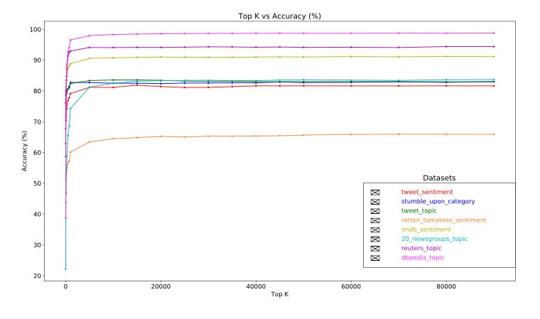
A more interesting finding is that for many datasets, we found that accuracy peaks at around 20,000 features for most datasets (see Figure 6). Adding new features above this threshold has little impact on the performance and sometimes even leads to overfitting and performance degradation as a result.
Normalization
When features/sample values are normalized, they are converted into small and similar values. In terms of convergent gradient descent algorithms, this simplifies the process of convergence. We have observed that normalizing data during data preprocessing does not seem to add much value to text classification problems. It is recommended that this step be skipped if the problem does not require it.
All of the above steps are put together in the following code:
Taking text samples and tokenizing them into word uni+bigrams,
Utilizing the TTF-IDF encoding, vectorize the image,
By discarding tokens that appear fewer than two times from the vector of tokens, and using f_classif to calculate the importance of individual features, we can identify the top 20,000 features from the vector of tokens.
It should be noted that when we represent words as n-gram vectors, we discard a great deal of information about word order and grammar (at best, we are able to preserve a fraction of the order information when n > 1). An approach based on a bag of words is sometimes referred to as a bag-of-words approach. There are several models that are using this representation, including logistic regression, multi-layer perceptrons, gradient boosting machines, and support vector machines, but these models don’t take order into account.
Sequence Vectors [Option B]
We will discuss tokenization and vectorization in the following paragraphs to show how we can do tokenization and vectorization for sequence models. It will also be covered how to use feature selection and normalization techniques in order to improve the representation of the sequence.
Word order can have a significant impact on the meaning of some text samples. As an example, let us take the sentence, “I used to hate the commute to work. It is only when you read the words in order that you can understand how my new bike has completely changed that.”. There are models available that can predict meaning based on the order in which words appear in the sample. This model represents the text as a sequence of tokens that are preserved in the order in which they appear in the text.
Tokenization
In the context of text, it is possible to represent a sequence of characters as well as a sequence of words. As a result, we found that word-level representations are more efficient than character tokens in terms of providing better performance. In addition to this, it is also the general trend that is followed by the industry in general. Using character tokens is not a good idea unless your texts have many typos in them, which is not the case in most cases.
Vectorization
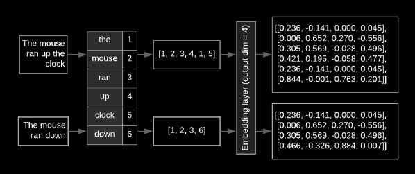
We are now in the process of converting our text samples into sequences of words that will then be converted into numerical vectors that can be analyzed. As shown in the example below, the indexes assigned to the unigrams generated from two texts have been shown as well as the sequence of token indexes to which the first text has been converted.
Token sequences can be vectorized in two ways:
Word vectors are used to represent sequences in n-dimensional space, where n is the vocabulary size. When tokenizing as characters with a small vocabulary, this representation works well. One-hot vectors are very sparse and inefficient when tokenizing as words with tens of thousands of tokens. Example:
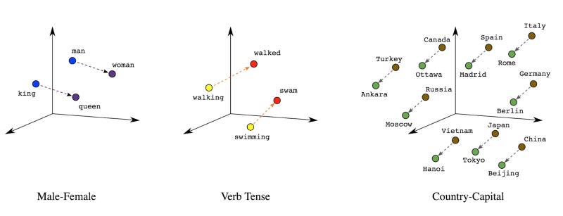
An embedding is a relationship between a word and its meaning(s). By representing word tokens as dense vector spaces (of a few hundred real numbers), we can determine how similar the words are semantically (Figure 7). A word embedding is a representation of this type.
There is often an embedding layer at the top of sequence models as the first layer of the model. During the training process, this layer learns how to convert word index sequences into word embedding vectors, so that each word index gets mapped to a dense vector of real values that reflect the location of that word in semantic space, following the training process (see figure 8).
Feature selection
Label predictions are not made for all words in our data. When we eliminate words that are rare or irrelevant from our vocabulary, we can optimize our learning process. The most frequent 20,000 features are generally sufficient, as we observe. As shown in Figure 6, this applies to n-gram models as well.
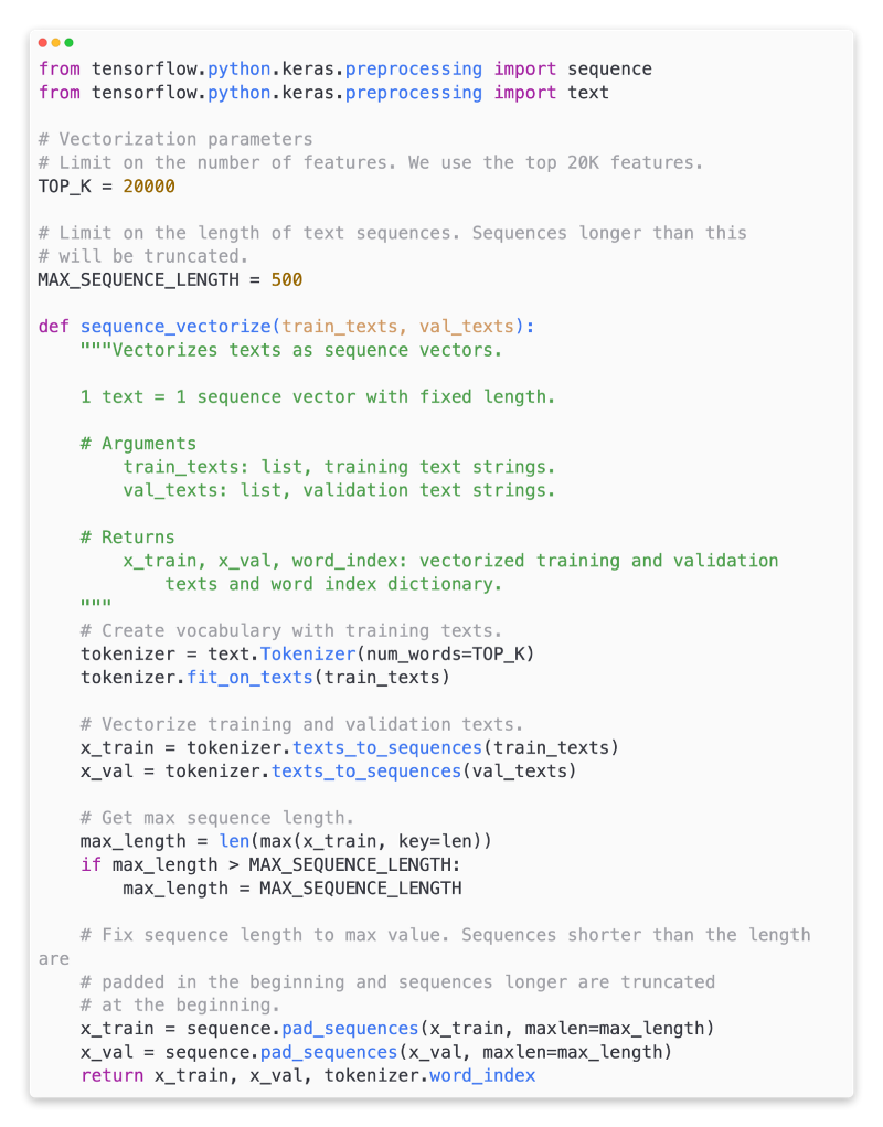
In sequence vectorization, let’s combine all the above steps. These tasks are performed by the following code:
Tokenizes the texts into words
Creates a vocabulary using the top 20,000 tokens
Converts the tokens into sequence vectors
Pads the sequences to a fixed sequence length
Label vectorization
A sample text data set was converted into a numerical vector. It is also necessary to apply the same process to the labels. It is simple to convert labels into values in the range [0, num_classes — 1]. In this case, we can just use the values 0, 1 and 2 to represent the three classes. To avoid inferring incorrect relationships between labels, the network will use one-hot vectors to represent these values. Our neural network uses a loss function and an activation function for its last layer to represent this information. Our next section will explain these in more detail.
Step 5: Build, Train, and Evaluate Your Model
Our goal in this section is to build, train, and evaluate our model. The fourth step involves choosing whether we want to use either a n-gram model or a sequence model, based on our S/W ratio. As soon as we have written our classification algorithm and trained it, we can proceed to the next step. In order to achieve this, we will be using TensorFlow with the tf.keras API provided by TensorFlow.
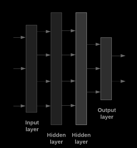
Building machine learning models is all about assembling layers of data-processing building blocks, much like assembling Lego bricks, which is exactly what we do when we build machine learning models using Keras. As a result of these layers, we are able to specify the sequence in which we want to perform the transformations on the input. Using the Sequential Model API we can create a line-by-line stack of layers from a single input text and an output classification that is calculated as a result of our learning algorithm.
Depending on whether we’re building an n-gram or a sequence model, the input layer and intermediate layers will vary based on how the input layer and intermediate layers will be constructed. It is important to note that regardless of the model type, the last layer for any given problem will remain the same.
Constructing the Last Layer
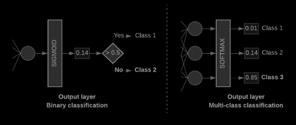
Our model should be able to produce a probability score if we have only two classes (binary classification). A probability score of 0.2 means that there is 20% confidence that a given input sample belongs to class 1 and 80% confidence that it belongs to class 0. This is possible by combining the activation function of the last layer with the loss function used to train the model.
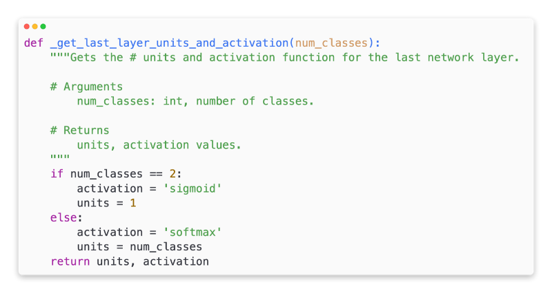
We should output one probability score per class when there are more than two classes. Summation should be 1. [0: 0.2, 1: 0.7, 2: 0.1] means 20% confidence that this sample is in class 0 and 70% confidence that it is in class 1 and 10% confidence that it is in class 2. It is recommended to use categorical cross-entropy as the loss function during training, and softmax as the activation function of the last layer. (See Figure 10, right).
Here is the code for a function that takes the number of classes as input and produces one unit for binary classification, and one unit for each class otherwise.
In the next two sections, we will explore how n-gram models and sequence models are constructed.
The n-gram model performs better than sequence models when the S/W ratio is small. Large numbers of small, dense vectors are better for sequence models. A dense space is the best place to learn embedding relationships, and this happens best after a large number of samples have been taken.

