


Understanding GRU and LSTM: Foundations for Deep Learning in Sequence Prediction
Understanding GRU and LSTM: Foundations for Deep Learning in Sequence Prediction
Bridging the Gap in Sequence Modeling with Recurrent Neural Networks

In the realm of deep learning, sequence prediction tasks stand out due to their complexity and the unique challenges they present. From predicting future stock prices to understanding natural language and forecasting weather patterns, the ability to predict sequential data accurately has vast applications across numerous fields. Central to solving these tasks are two powerful neural network architectures: Gated Recurrent Units (GRU) and Long Short-Term Memory (LSTM) units.
The Essence of Recurrent Neural Networks (RNNs)
Before delving into GRU and LSTM, it’s crucial to understand the foundation upon which they are built: Recurrent Neural Networks (RNNs). RNNs are designed to recognize patterns in sequences of data by maintaining a ‘memory’ of previous inputs in their internal state. This feature makes RNNs ideally suited for tasks involving sequential data, such as time series analysis, language modeling, and speech recognition.
However, standard RNNs are plagued by challenges like vanishing and exploding gradients, making it difficult for them to learn long-range dependencies within the data. This is where GRU and LSTM units come into play, offering sophisticated mechanisms to capture such dependencies effectively.
Long Short-Term Memory (LSTM) Units
Developed to overcome the limitations of traditional RNNs, LSTM units incorporate a series of gates (input, output, and forget gates) that regulate the flow of information. These gates determine what information should be retained or discarded at each step, allowing the network to maintain a long-term memory. LSTMs are highly effective in scenarios where the relationship between distant points in the sequence is crucial for accurate predictions.
Gated Recurrent Units (GRU)
GRU is a more recent innovation designed to simplify the LSTM model while retaining its ability to learn long-range dependencies. GRUs merge the forget and input gates into a single update gate and blend the cell state and hidden state, thereby reducing the complexity of the model. This simplification often leads to faster training times and comparable, if not superior, performance on certain tasks.
Choosing Between GRU and LSTM
The decision to use GRU or LSTM largely depends on the specific requirements of the task and the dataset at hand. GRUs offer a simpler architecture and may outperform LSTMs on datasets where long-term dependencies are less critical. Conversely, LSTMs provide a more nuanced control over the memory and might excel in tasks with complex temporal relationships.
Download the source code from the link at the end of this article.
Install libraries and set up neural network.
!pip install tensorflow
!pip install keras
import pandas as pd
import numpy as np
import tensorflow as tf
import matplotlib.pyplot as plt
from sklearn.preprocessing import MinMaxScaler
from sklearn.model_selection import train_test_split
from tensorflow.keras.preprocessing.sequence import TimeseriesGenerator
from tensorflow.keras.models import Sequential, load_model
from tensorflow.keras.layers import SimpleRNN, Dense
from tensorflow.keras.layers import GRU
The installation of necessary Python packages using pip, a package installer for Python.
To install the TensorFlow library, a popular open-source machine learning framework developed by Google for building deep learning models, the command is ‘pip install tensorflow’.
To install the Keras library, a high-level neural networks API that can run on top of TensorFlow or other deep learning frameworks, the command is ‘pip install keras’.
These libraries are crucial for developing and training deep learning models. Additionally, the code imports various modules such as pandas, numpy, tensorflow, matplotlib, and components from the TensorFlow Keras API to aid in tasks such as data manipulation, model building, and visualization.
Reads and displays a CSV file.
data = pd.read_csv("indexProcessed.csv", sep=",")
data
We can read a CSV file named “indexProcessed.csv” into a pandas DataFrame by using the pd.read_csv() function. The sep=”,” parameter is used to specify that the values in the CSV file are separated by commas.
This process is crucial as it enables us to import a structured dataset from a CSV file into a format that can be efficiently handled and analyzed using the robust functionalities of the pandas library in Python. By loading the data into a DataFrame, we can conduct tasks such as data cleaning, manipulation, exploratory data analysis, and more, allowing us to extract insights and make informed decisions based on the data.
Prints information about the dataset.
data.info()<class 'pandas.core.frame.DataFrame'>
RangeIndex: 104224 entries, 0 to 104223
Data columns (total 9 columns):
# Column Non-Null Count Dtype
--- ------ -------------- -----
0 Index 104224 non-null object
1 Date 104224 non-null object
2 Open 104224 non-null float64
3 High 104224 non-null float64
4 Low 104224 non-null float64
5 Close 104224 non-null float64
6 Adj Close 104224 non-null float64
7 Volume 104224 non-null float64
8 CloseUSD 104224 non-null float64
dtypes: float64(7), object(2)
memory usage: 7.2+ MBThe data.info() method in Python is commonly used with pandas DataFrames to give a brief summary of the data. It includes information like column names, non-null value counts, data types of columns, and memory usage of the DataFrame.
By utilizing data.info(), analysts and scientists can gain insights into the data’s structure, including data types and missing values. This knowledge aids in making informed decisions on data preprocessing and analysis.
Summarizes statistics of the data.
data.describe()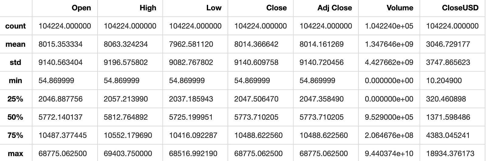
The describe() function in pandas generates descriptive statistics of the data, including count, mean, standard deviation, minimum, maximum, and quartile values. It summarizes the central tendency, dispersion, and shape of the dataset’s distribution. This function aids in comprehending the distribution of numerical data, identifying outliers, and quickly grasping the dataset’s characteristics.
Count missing values in each column.
data.isna().sum()Index 0
Date 0
Open 0
High 0
Low 0
Close 0
Adj Close 0
Volume 0
CloseUSD 0
dtype: int64To determine the number of missing values (NaN) in each column of a dataset, this process involves using a boolean mask generated by calling data.isna(). True in the mask indicates a missing value and False indicates a non-missing value. By applying .sum() to this mask, the code calculates the count of True values, which signifies the number of missing values in each dataset column.
Utilizing this code is crucial when dealing with datasets to address issues that missing values can introduce to data analysis and modeling. Identifying and managing missing values correctly is essential for maintaining the reliability and precision of analyses and decision-making procedures.
Prepare the data for analysis.
Sets random number generator seeds.
np.random.seed(42)
tf.random.set_seed(24)
This snippet establishes the seed value for the random number generators in two libraries: NumPy and TensorFlow.
By setting the seed, a consistent sequence of random numbers is produced, enabling reproducibility of results. This is particularly advantageous when wanting to maintain consistency across multiple executions of the program.
Here, the NumPy seed is designated as 42 and the TensorFlow seed as 24. Consequently, functions from these libraries will consistently generate the same random numbers when the code is executed using these specific seed values. This predictability is helpful for debugging, testing, and ensuring the reliability of outcomes in machine learning models.
Check the data type of the first date.
type(data.Date[0])strThis snippet retrieves the data type of the element at index 0 in the ‘Date’ column of the ‘data’ dataset. Understanding the data type is important for handling data properly, including sorting, filtering, and performing mathematical operations. This information is crucial for data analysis and processing tasks to make well-informed decisions.
Converts date column to datetime format.
data["Date"] = pd.to_datetime(data["Date"])
display(data.dtypes)
display(data[["Date"]].sample(5))
Index object
Date datetime64[ns]
Open float64
High float64
Low float64
Close float64
Adj Close float64
Volume float64
CloseUSD float64
dtype: objectThis process converts the “Date” column in a pandas DataFrame into datetime format using the pd.to_datetime() function from the pandas library. This conversion ensures that dates are correctly interpreted as dates, making manipulation and analysis of date-based data easier.
After the conversion, the code displays the data types of all columns in the DataFrame to confirm the success of the conversion. It also shows a random sample of 5 rows from the “Date” column to demonstrate the effect of the conversion.
Converting date columns to datetime format is crucial for working with date-based data. It ensures that dates are handled correctly for operations like filtering, grouping, and plotting based on dates. This conversion also helps prevent potential errors that can occur when working with dates in string format. Overall, converting date columns to datetime format enhances the accuracy and efficiency of data analysis.
Find unique values in Index column.
data.Index.unique()array(['HSI', 'NYA', 'IXIC', '000001.SS', 'N225', 'N100', '399001.SZ',
'GSPTSE', 'NSEI', 'GDAXI', 'SSMI', 'TWII', 'J203.JO'], dtype=object)This method is used to extract the unique values from the “Index” column in a dataset. It provides an array-like object that contains all the distinct values found in the “Index” column. This can aid in identifying different categories or groups represented in the dataset, or to recognize unique identifiers within the data.
Utilizing this approach is crucial when analyzing the unique values within a column without repetitions. It proves beneficial for tasks such as data exploration, data cleansing, and gaining insights into the variety of values existing in the dataset.
The code plots close prices of indices.
grouped = data.groupby('Index')
plt.figure(figsize=(20, 10))
for stock, info in grouped:
    plt.plot(info['Date'], info['CloseUSD'], label=stock)
plt.xlabel('Date')
plt.ylabel('Close Price')
plt.legend()
plt.title('Index Prices in USD')
plt.xticks(rotation=45)
plt.show()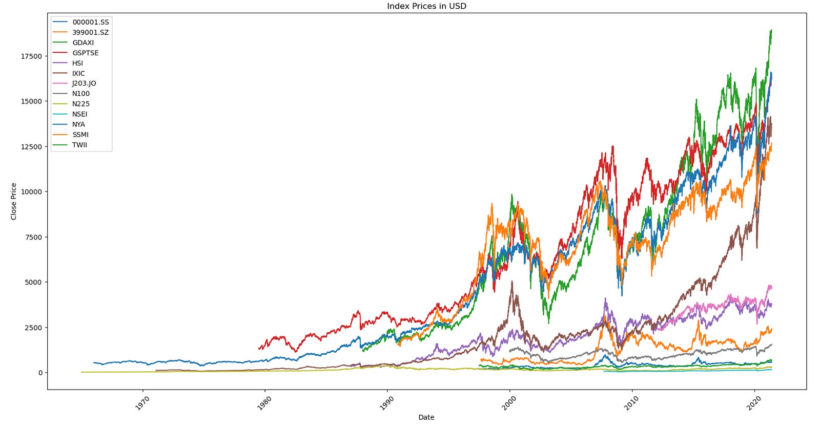
This method visualizes the closing prices of various stocks over time using a line plot. Here’s an overview of how it functions:
Data is grouped based on the ‘Index’ column.
A matplotlib figure is generated with dimensions of 20x10 inches.
For each group of stocks (grouped by ‘Index’), a line plot is created, with ‘Date’ on the x-axis and ‘CloseUSD’ on the y-axis. Each line represents the closing price of a different stock, with the stock name as a label.
The x-axis is labeled as ‘Date’, and the y-axis as ‘Close Price’.
A legend is included on the plot to distinguish between the stocks.
The plot title is set to ‘Index Prices in USD’.
X-axis tick labels are rotated by 45 degrees for improved readability.
Finally, the plot is shown using plt.show().
This code is crucial for visualizing and comparing the closing prices of various stocks over time. It aids in recognizing trends, patterns, and relationships among stock prices of different companies within the same index. By graphing this data, analysts and investors can make well-informed decisions regarding their investment strategies.
Filter and copy data based on different indices.
N100 = data[data['Index'] == "N100"].copy()
HSI = data[data['Index'] == "HSI"].copy()
NYA = data[data['Index'] == "NYA"].copy()
IXIC = data[data['Index'] == "IXIC"].copy()
N225 = data[data['Index'] == "N225"].copy()
GSPTSE = data[data['Index'] == "GSPTSE"].copy()
NSEI = data[data['Index'] == "NSEI"].copy()
GDAXI = data[data['Index'] == "GDAXI"].copy()
SSMI = data[data['Index'] == "SSMI"].copy()
TWII = data[data['Index'] == "TWII"].copy()
SSE = data[data['Index'] == "000001.SS"].copy()
JSE = data[data['Index'] == "J203.JO"].copy()
SZSE = data[data['Index'] == "399001.SZ"].copy()
This method involves creating individual dataframes for various stock indices by sorting the ‘data’ dataframe according to the ‘Index’ column. Each dataframe includes data specific to a particular stock index like N100, HSI, NYA, and others.
This approach aids in organizing and managing data associated with distinct stock indices separately. By establishing separate dataframes for each stock index, it simplifies the analysis and manipulation of data for each index individually. This can facilitate a more efficient comparison of performance, trends, and other features among different stock indices.
Sets index to “Date”, selects 5 random rows.
HSI.set_index("Date", inplace=True)
HSI.sample(5)
The “Date” column is set as the index of the DataFrame HSI using the set_index() method with inplace=True. This directly modifies the original DataFrame, and the method returns None.
After setting the “Date” column as the index, 5 rows are randomly selected from the DataFrame for inspection using the sample() method.
Setting the index to a specific column is common in time-series or data with meaningful index information, enabling easier manipulation, analysis, and visualization based on the index values. By setting the “Date” column as the index, data based on specific dates can be easily accessed, and the index used for various DataFrame operations. The sample() method helps to randomly select rows for analysis or exploration.
Copies “CloseUSD” values, checks shape.
closed_HSI = HSI[["CloseUSD"]].copy()
closed_HSI.shape
(8492, 1)This snippet extracts the “CloseUSD” column from a DataFrame named HSI, saves it as closed_HSI, and then retrieves the dimensions of the new DataFrame using the shape attribute.
It’s a common practice in data analysis to make a copy of a specific column for further manipulation or analysis to avoid altering the original data. The shape attribute provides an overview of the DataFrame’s dimensions.
Exploring Data
Display information about closed_HSI dataframe.
closed_HSI.info()<class 'pandas.core.frame.DataFrame'>
DatetimeIndex: 8492 entries, 1986-12-31 to 2021-05-31
Data columns (total 1 columns):
# Column Non-Null Count Dtype
--- ------ -------------- -----
0 CloseUSD 8492 non-null float64
dtypes: float64(1)
memory usage: 132.7 KBThe closed_HSI.info() function in Python is commonly used with the Pandas library to retrieve information about the data stored in the “closed_HSI” DataFrame. It offers a brief overview of the DataFrame, presenting details such as column names, data types, the count of non-null values in each column, and memory consumption.
Utilizing this function allows for a swift examination of the dataset’s layout, detection of any absent values, comprehension of the data types in each column, and an understanding of memory usage. Such insights are crucial for tasks like data cleansing, processing, analysis, and visualization.
Describes statistics of closed_HSI dataset.
closed_HSI.describe()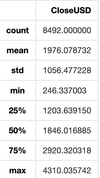
The describe() function in pandas is utilized for generating descriptive statistics of a DataFrame. By using closed_HSI.describe(), you can access statistics including count, mean, standard deviation, minimum, 25th percentile (Q1), median (50th percentile), 75th percentile (Q3), and maximum for each numerical column in the closed_HSI DataFrame. These statistics aid in grasping the data distribution within the DataFrame, encompassing central tendency, dispersion, and quartiles. It serves as a valuable tool for data exploration and obtaining immediate insights into the data.
Summary: Describes a dataset.
closed_HSI.describe()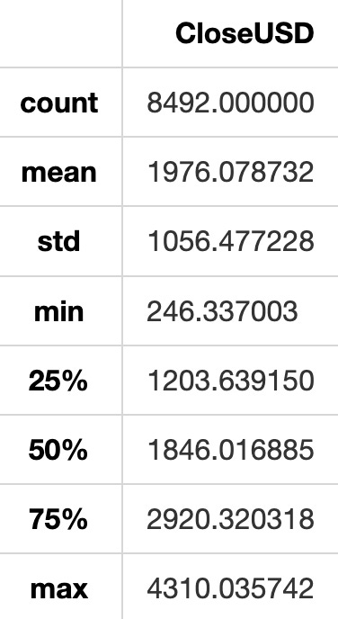
The closed_HSI.describe() function generates a summary of descriptive statistics for the data in the variable closed_HSI. It provides statistics like count, mean, standard deviation, minimum, maximum, and quartile values.
This function is helpful for quickly grasping an overview of the data’s distribution without checking each individual data point. It aids in identifying outliers, understanding the data’s range of values, and central tendency.
In essence, describe() is a convenient tool for gaining insights into the data and better understanding its features.