

Understanding time series forecasting
Time series forecasting is a specialized area of data analysis and machine learning focused on predicting future values of a variable based on its past observations.

Unlike other statistical or machine learning tasks that assume independence between data points, time series data inherently possesses a temporal order, meaning the sequence of observations is crucial and carries significant information.
Link To Download Source Code & Dataset At the end of article!
What is a Time Series?
A time series is a sequence of data points indexed, or listed, in time order. Most commonly, a time series is a sequence taken at successive equally spaced points in time. Examples include daily stock prices, hourly temperature readings, monthly sales figures, or yearly population counts. The defining characteristic is that each data point is associated with a specific timestamp.
Consider a simple example: tracking the daily closing price of a particular stock. Each day, we record a single value, and these values, when ordered by date, form a time series.
Let’s illustrate this with a simple synthetic time series using Python. We’ll generate a series representing daily temperature over a month.
import pandas as pd
import numpy as np
import matplotlib.pyplot as plt
# Set a random seed for reproducibility
np.random.seed(42)
We begin by importing the necessary libraries: pandas for data manipulation, numpy for numerical operations (like generating random data), and matplotlib.pyplot for plotting. Setting a random seed ensures that our synthetic data will be the same every time you run the code, which is helpful for consistent examples.
# Create a date range for 30 days
dates = pd.date_range(start='2023-01-01', periods=30, freq='D')
# Generate synthetic temperature data with a slight trend and noise
# Base temperature around 20 degrees, add a small increasing trend
# Add some random fluctuations (noise)
temperatures = 20 + np.arange(30) * 0.1 + np.random.normal(0, 1.5, 30)
Here, we create our time index using pd.date_range for 30 consecutive days starting from January 1, 2023. For the temperature data, we simulate a realistic scenario by starting with a base temperature, adding a slight linear increase over the 30 days (representing a subtle trend), and then incorporating random noise using np.random.normal to mimic real-world variability.
# Create a Pandas Series with dates as the index
daily_temperatures = pd.Series(temperatures, index=dates, name='Temperature')
# Display the first few entries to see the structure
print("First 5 entries of the daily temperature time series:")
print(daily_temperatures.head())
We then combine our generated temperatures and dates into a pandas.Series. A pandas.Series is an excellent data structure for time series data because it automatically handles the time index, making subsequent operations like plotting or resampling much easier. Printing the head of the series shows how the date acts as the index for each temperature reading.
# Plot the time series
plt.figure(figsize=(10, 6))
daily_temperatures.plot(title='Daily Temperature Time Series (Synthetic Data)',
                         xlabel='Date',
                         ylabel='Temperature (°C)',
                         grid=True)
plt.show()
Finally, we visualize our synthetic time series. Plotting a time series is crucial for initial exploration, allowing us to observe patterns like trends, seasonality, and irregular fluctuations. The x-axis represents time, and the y-axis represents the observed value. This simple line plot clearly illustrates the temporal progression of the data.
The Purpose of Time Series Forecasting
The primary purpose of time series forecasting is to make informed decisions about the future. By predicting how a variable will behave over time, businesses, governments, and researchers can:
Optimize Resource Allocation: Forecast demand for products to manage inventory, schedule staffing, or plan production.
Mitigate Risks: Predict financial market volatility or potential equipment failures to take proactive measures.
Inform Policy and Strategy: Forecast economic indicators (GDP, inflation) for policy-making, or predict disease spread for public health interventions.
Understand Underlying Dynamics: Analyzing past patterns can reveal insights into the processes generating the data.
Practical applications span various domains:
Business & Finance: Sales forecasting, stock price prediction, energy consumption forecasting, call center staffing.
Meteorology: Weather forecasting, climate modeling.
Econometrics: Predicting GDP, unemployment rates, inflation.
Industrial Processes: Predictive maintenance for machinery, quality control.
Marketing: Forecasting ad campaign effectiveness, website traffic.
Healthcare: Predicting patient admissions, disease outbreaks.
Time Series Forecasting vs. Other Regression Tasks: Key Distinctions
While forecasting involves predicting a numerical value, much like a standard regression problem (e.g., predicting house prices based on features like size, location, number of bedrooms), there are fundamental differences that necessitate specialized techniques for time series data. Ignoring these distinctions can lead to flawed models and inaccurate predictions.
Temporal Dependence (Autocorrelation):
Standard Regression: Assumes that observations are independent of each other. The prediction for one house price doesn’t directly depend on another house’s price in the training set (beyond shared features).
Time Series Forecasting: The most critical distinction is temporal dependence. The value at time
tis highly dependent on values att-1,t-2, and so on. This inherent correlation between successive observations is called autocorrelation. For example, today's temperature is very likely related to yesterday's temperature.
Order Matters:
Standard Regression: The order of rows in your dataset typically doesn’t matter. If you shuffle the rows of a house price dataset, the model will still learn the same relationships.
Time Series Forecasting: The chronological order of data points is paramount. Shuffling a time series destroys its inherent temporal structure and makes it impossible to forecast. Models must respect this sequence.
Future Prediction Only:
Standard Regression: Often used to estimate relationships between variables or predict existing outcomes (e.g., predicting the price of a house currently on the market). All features used for prediction are known at the time of prediction.
Time Series Forecasting: The goal is to predict future values of the variable itself. This means that any features used for prediction (exogenous variables) must also be known for the future, or themselves be forecasted.
Stationarity:
Standard Regression: Assumes that the underlying data-generating process is stable.
Time Series Forecasting: Many time series exhibit non-stationary behavior, meaning their statistical properties (like mean, variance, or autocorrelation) change over time. For example, a company’s sales might have an increasing trend over years. Many traditional time series models require the series to be stationary (or transformed to be so) for valid inference and accurate forecasting.
Components of a Time Series
To better understand the patterns within a time series, it’s often helpful to decompose it into several underlying components. While we’ll delve into decomposition methods later, a high-level understanding is crucial from the outset:
Trend (T): This represents the long-term increase or decrease in the data over time. It’s the overall direction of the series, ignoring short-term fluctuations. For example, the growing global population exhibits an upward trend. In our synthetic temperature example, we added a slight upward trend.
Seasonality (S): These are regular, repeating patterns or cycles in the data that occur at fixed and known intervals. For instance, retail sales often peak during holidays, or electricity consumption might peak during certain hours of the day or seasons of the year. The length of a cycle is called the seasonal period (e.g., 7 days for weekly seasonality, 12 months for annual seasonality).
Residuals / Noise (R): Also known as the “remainder” or “irregular” component, this is what’s left after accounting for the trend and seasonal components. It represents the random, unpredictable fluctuations in the data that cannot be explained by trend or seasonality. This is often the part we aim to minimize in our models.
These components can be combined additively (e.g., Y = T + S + R) or multiplicatively (e.g., Y = T * S * R), depending on whether the magnitude of the seasonal fluctuations changes with the level of the series.
Python’s Prominence in Time Series Analysis
Python has emerged as the dominant programming language for data science, machine learning, and consequently, time series analysis and forecasting. Its popularity stems from several key advantages:
Versatility: Python is a general-purpose language, meaning it’s not limited to statistical computing. You can use it for data cleaning, web development, deploying models, and building entire applications, providing an end-to-end solution.
Rich Ecosystem of Libraries: Python boasts an incredibly extensive collection of open-source libraries specifically designed for data manipulation, statistical analysis, machine learning, and deep learning.
pandas: Indispensable for data manipulation, especially with time-indexed data.NumPy: Provides powerful numerical computing capabilities.MatplotlibandSeaborn: For data visualization.SciPy: A collection of scientific computing tools.statsmodels: Offers a wide array of statistical models, including classical time series models like ARIMA, ETS, and state-space models.scikit-learn: A comprehensive machine learning library with tools for regression, classification, clustering, and more, which can be adapted for time series feature engineering.Specialized Libraries: Libraries like
Prophet(developed by Facebook) andpmdarima(auto-ARIMA) streamline common forecasting tasks.Deep Learning Frameworks:
TensorFlowandPyTorchenable the development of advanced neural network models, including Recurrent Neural Networks (RNNs) and Transformers, which are highly effective for complex time series patterns.Community Support: A large and active community means abundant resources, tutorials, and quick resolution of issues.
Readability: Python’s syntax is often described as clear and intuitive, making it easier to learn and write maintainable code.
While languages like R have historically been strong in statistical computing, Python’s broader applicability and its robust machine learning and deep learning ecosystem make it the preferred choice for modern time series forecasting, especially when integrating with larger data pipelines or deploying models into production. This book will leverage Python extensively, providing practical, hands-on examples that build your proficiency in this powerful environment.
Pedagogical Progression of This Book
This book is structured to guide you through the exciting world of time series forecasting in a logical and progressive manner. We will begin with foundational concepts and simpler statistical models, gradually building complexity as we introduce more advanced techniques.
You will start by understanding the basic characteristics of time series data and classic statistical methods like Exponential Smoothing and ARIMA models, which form the bedrock of many forecasting solutions. As your understanding deepens, we will transition to machine learning approaches, where you’ll learn to engineer features from time series data and apply powerful algorithms. Finally, we will explore the cutting edge of time series forecasting with deep learning models, leveraging the capabilities of neural networks to capture intricate temporal dependencies and long-term patterns. This structured approach ensures that you build a strong conceptual and practical foundation, enabling you to tackle a wide range of real-world forecasting challenges.
What is a Time Series?
At its core, a time series is a sequence of data points indexed, or listed, in time order. This means that each data point in the series corresponds to a specific point in time, and the order of these points is crucial. Unlike other forms of data analysis where observations might be independent or arbitrarily ordered, in time series analysis, the temporal sequence is the primary independent variable and carries significant information.
Consider the daily closing price of a stock, the quarterly earnings of a company, or the hourly temperature readings from a sensor. In each case, the value observed at one point in time is often influenced by, and provides context for, values observed at previous points in time. This inherent temporal dependency is what fundamentally distinguishes time series data from other types of datasets, such as cross-sectional data (e.g., a survey of customer preferences at a single point in time) or panel data (which combines cross-sectional observations over time but often treats time as a separate dimension rather than the primary index).
Defining Characteristics of Time Series Data
While the definition is straightforward, understanding the nuances of time series data is key to effective analysis and forecasting.
Time-Ordered Sequence
The most critical characteristic is that the data points are ordered by time. This is not merely a convenience; it is a fundamental property. Changing the order of observations in a time series would fundamentally alter its meaning and the patterns it exhibits. For instance, scrambling the order of daily stock prices would render the data meaningless for financial analysis, as the progression of prices over time is what reveals trends, volatility, and market cycles.
Often Equally Spaced Intervals
Many time series, especially those amenable to traditional forecasting models, consist of observations taken at regular, equally spaced intervals. Examples include:
Hourly: Temperature readings, website traffic.
Daily: Stock prices, sales figures.
Weekly: Retail sales, energy consumption.
Monthly: Unemployment rates, inflation data.
Quarterly: Company earnings, GDP figures.
Annually: Population growth, agricultural yields.
The assumption of equally spaced data simplifies the application of many time series models, as it implies a consistent underlying sampling frequency.
However, it’s important to acknowledge that not all real-world time series are equally spaced. Data from event logs, irregular sensor readings (where data is only transmitted upon significant change), or financial trade data (where transactions occur at irregular intervals) are examples of unequally spaced or irregular time series. While this book will primarily focus on equally spaced time series due to their prevalence in many business and economic applications and the simpler modeling approaches, be aware that specialized techniques exist for handling irregular data, often involving resampling, interpolation, or event-based modeling.
Temporal Dependencies and Autocorrelation
A defining feature of time series is that observations are typically not independent of each other. The value at the current time point often depends on values from previous time points. This phenomenon is known as autocorrelation — the correlation of a variable with itself over different time lags. For example, today’s stock price is highly correlated with yesterday’s price, and last month’s sales figures are likely to influence this month’s sales. This temporal dependency is precisely why traditional regression models, which often assume independent observations, are insufficient for time series forecasting. Time series models are specifically designed to capture and leverage these internal dependencies to make accurate predictions.
Representing Time Series Programmatically: The Time Index
When working with time series data in Python, especially with the powerful pandas library, the concept of the "time index" becomes paramount. pandas DataFrames and Series are ideal for handling time series because they allow for a dedicated DatetimeIndex. This index is not just a label; it's a specialized data type that enables powerful time-based operations like resampling, slicing by date ranges, and frequency analysis.
Let’s look at a simple example of how a time series might be structured in pandas.
import pandas as pd
# 1. Define a sequence of dates (our time index)
# We'll create daily dates for a week starting from January 1, 2023
dates = pd.to_datetime(['2023-01-01', '2023-01-02', '2023-01-03', '2023-01-04',
                        '2023-01-05', '2023-01-06', '2023-01-07'])
# 2. Define a sequence of values (our data points)
# Let's imagine these are daily website visitors
website_visitors = [1200, 1350, 1100, 1500, 1600, 1800, 1750]
# 3. Create a pandas Series with the dates as the index
# This is a fundamental way to represent a time series in Python
daily_visitors_ts = pd.Series(website_visitors, index=dates)
# Display the time series
print(daily_visitors_ts)
This first code chunk demonstrates how to create a basic time series using pandas. We define a list of dates, convert them into datetime objects suitable for a pandas index using pd.to_datetime(), and then pair them with a corresponding list of values. The pd.Series() constructor, when given both data and an index, automatically creates a time series where the dates serve as the explicit time-ordered labels for each data point.
# Check the type of the index to confirm it's a DatetimeIndex
print("\nType of index:", type(daily_visitors_ts.index))
print("Data type of index elements:", daily_visitors_ts.index.dtype)
This small addition verifies that pandas correctly recognized our dates and assigned a DatetimeIndex. This specialized index type is what unlocks pandas's powerful time series capabilities, allowing for efficient operations like selecting data by date ranges or resampling data to different frequencies (e.g., converting daily data to weekly averages).
Real-World Examples of Time Series
Time series data is ubiquitous across virtually every domain. Recognizing these patterns in various contexts is the first step towards applying time series forecasting techniques.
Financial Markets:
Stock Prices: Daily, hourly, or even minute-by-minute closing prices, opening prices, high/low values for individual stocks or market indices (e.g., S&P 500).
Exchange Rates: Fluctuations of currency pairs (e.g., USD/EUR) over time.
Company Earnings: Quarterly or annual earnings per share, revenue, or profit figures.
Interest Rates: Daily or monthly changes in benchmark interest rates.
Economic Indicators:
Gross Domestic Product (GDP): Quarterly or annual economic output of a country.
Inflation Rates: Monthly or annual percentage change in consumer prices.
Unemployment Rates: Monthly percentage of the labor force that is unemployed.
Consumer Price Index (CPI): Monthly measure of the average change over time in the prices paid by urban consumers for a market basket of consumer goods and services.
Environmental and Climate Data:
Temperature Readings: Hourly, daily, or monthly average temperatures in a specific location.
Rainfall/Precipitation: Daily or monthly accumulated rainfall.
Air Quality: Hourly measurements of pollutants like PM2.5 or ozone.
Ocean Levels: Annual measurements of sea level rise.
Business and Retail:
Sales Data: Daily, weekly, or monthly sales volumes for products or services.
Website Traffic: Hourly or daily unique visitors, page views, or conversion rates.
Customer Service Calls: Number of calls received per hour or day.
Inventory Levels: Daily or weekly counts of goods in stock.
Healthcare and Medical:
EKG/ECG Readings: Continuous measurements of electrical activity of the heart.
Blood Pressure Monitoring: Hourly or daily readings for patients.
Disease Incidence: Weekly or monthly counts of new disease cases (e.g., flu outbreaks).
Internet of Things (IoT) and Sensor Data:
Smart Home Devices: Energy consumption, temperature, or humidity readings from connected devices.
Industrial Sensors: Pressure, temperature, vibration data from machinery for predictive maintenance.
Vehicle Telemetry: Speed, location, engine performance data over time.
This diverse range of examples underscores the universality of time series data and the broad applicability of forecasting techniques across various industries and scientific disciplines.
Introducing the Johnson & Johnson Earnings Dataset
Throughout this book, we will frequently refer to and analyze the Johnson & Johnson (J&J) quarterly earnings per share (EPS) dataset. This dataset is a classic example in time series analysis due to its clear and illustrative patterns. It tracks the quarterly earnings per share for the pharmaceutical and consumer goods giant Johnson & Johnson from 1960 to 1980.
Let’s load this dataset (or a similar representative one for illustration) and visualize it to understand its key properties. For this introductory section, we will use a simplified approach to loading data, assuming it’s available in a common format like a CSV file.
import matplotlib.pyplot as plt
import pandas as pd
# Load the Johnson & Johnson earnings dataset
# Assuming 'jj_earnings.csv' is in the same directory
# The 'Quarter' column contains dates, and 'Earnings' contains the EPS values.
try:
jj_data = pd.read_csv('data/jj_earnings.csv', index_col='Quarter', parse_dates=True)
except FileNotFoundError:
print("jj_earnings.csv not found. Please ensure the data file is in the 'data' directory.")
# Create a synthetic dataset if the real one isn't available for demonstration
dates = pd.to_datetime(pd.date_range(start='1960-01-01', periods=84, freq='QS-OCT')) # Quarterly start, Oct for Q4
earnings = [
0.71, 0.63, 0.85, 0.44, 0.61, 0.69, 0.92, 0.55, 0.72, 0.77, 0.92, 0.60,
0.83, 0.80, 1.00, 0.67, 0.92, 0.95, 1.05, 0.76, 1.03, 1.08, 1.21, 0.88,
1.16, 1.25, 1.45, 1.05, 1.30, 1.45, 1.74, 1.25, 1.55, 1.60, 2.07, 1.62,
1.71, 1.86, 2.36, 1.70, 1.91, 2.15, 2.79, 2.00, 2.22, 2.50, 3.23, 2.37,
2.60, 2.90, 3.65, 2.80, 3.10, 3.50, 4.30, 3.40, 3.60, 4.00, 4.96, 4.00,
4.30, 4.70, 5.70, 4.60, 5.30, 6.00, 7.20, 6.00, 7.10, 8.50, 10.00, 9.00,
10.00, 11.50, 13.00, 12.00, 14.00, 16.00, 18.00, 20.00, 23.00, 26.00, 30.00, 35.00
]
jj_data = pd.Series(earnings, index=dates, name='Earnings')
jj_data = pd.DataFrame(jj_data) # Convert to DataFrame for consistency
print("Using synthetic J&J-like data for demonstration.")# Display the first few rows of the dataset
print("First 5 rows of Johnson & Johnson Earnings:")
print(jj_data.head())This code snippet prepares the J&J dataset for analysis. It attempts to load a CSV file, which is a common way to obtain real-world data. Crucially, index_col='Quarter' and parse_dates=True tell pandas to use the 'Quarter' column as the DatetimeIndex, ensuring the data is correctly recognized as a time series. A fallback synthetic dataset is included for robustness, allowing the code to run even if the specific CSV isn't present, mimicking the real data's characteristics. Displaying .head() allows us to quickly inspect the structure and ensure the time index is correctly set.
Now, let’s visualize the data:
# Plot the time series
plt.figure(figsize=(12, 6)) # Set the figure size for better readability
plt.plot(jj_data.index, jj_data['Earnings'], marker='o', linestyle='-', markersize=4)
plt.title('Johnson & Johnson Quarterly Earnings Per Share (1960-1980)')
plt.xlabel('Year')
plt.ylabel('Earnings Per Share ($)')
plt.grid(True) # Add a grid for easier reading of values
plt.xticks(rotation=45) # Rotate x-axis labels for better visibility
plt.tight_layout() # Adjust layout to prevent labels from overlapping
plt.show()
This plotting code uses matplotlib to generate a line plot, which is the standard way to visualize a time series. The jj_data.index (our DatetimeIndex) is used for the x-axis, and the 'Earnings' column for the y-axis. Markers and line styles are added for clarity, and standard plotting enhancements like titles, labels, and a grid are applied to make the visualization informative.
Visual Properties of the J&J Dataset
Upon examining the plot of the Johnson & Johnson earnings, several key characteristics become immediately apparent:
Trend: There is a clear upward trend over the entire period. Earnings per share generally increased from 1960 to 1980, indicating consistent growth for the company. This suggests that future earnings are likely to be higher than past earnings, a critical piece of information for forecasting.
Cyclical/Seasonal Behavior: Within each year, there’s a distinct pattern. Earnings tend to be lower in the first quarter (Q1) and then peak in the fourth quarter (Q4). This repeating pattern within a fixed period (a year, in this case) is known as seasonality. For a business, this often reflects seasonal demand for products, holiday sales, or fiscal reporting cycles.
Increasing Variability: As time progresses and the overall earnings increase, the magnitude of the seasonal fluctuations also appears to increase. The peaks and troughs become more pronounced in later years. This suggests that the variance (or standard deviation) of the series is not constant over time, a property known as heteroscedasticity. This is an important consideration for more advanced forecasting models.
These visual properties — trend, seasonality, and changing variability — are common in many real-world time series and will be central to the forecasting techniques explored in later sections.
Why is Time Series Forecasting Different?
You might wonder why we need specialized techniques for time series forecasting when standard regression methods can predict a dependent variable based on independent variables. The crucial distinction lies in the temporal dependence we discussed earlier.
In typical regression problems, observations are often assumed to be independent and identically distributed (i.i.d.). This means that the value of one observation does not influence another, and all observations come from the same underlying distribution. However, for time series data, this assumption is fundamentally violated.
The past values of a time series directly influence its future values. This inherent autocorrelation means that simply using time as an independent variable in a standard linear regression model often fails to capture the complex temporal dynamics. Such models might provide a general trend but would likely miss crucial patterns like seasonality or the impact of recent fluctuations. Time series forecasting models are specifically designed to explicitly account for these dependencies, leveraging the rich information contained within the sequence of observations to make more accurate and robust predictions.
Components of a Time Series
Time series data, by its very nature, is a collection of observations recorded over time. While a simple line plot can show the overall movement, a deeper understanding often requires us to break down the series into its fundamental building blocks. This process, known as time series decomposition, helps us identify and isolate the distinct patterns that contribute to the observed data. Understanding these components is crucial for diagnosing the behavior of a series, making informed forecasting decisions, and developing robust models.
The Observed Time Series
Before diving into components, let’s establish what we mean by the “observed time series.” This is simply the raw, actual data points collected over time, often denoted as $Y_t$, where $t$ represents a specific point in time. For instance, the monthly sales figures for a retail store, the daily temperature readings in a city, or the hourly electricity consumption of a building are all observed time series.
Trend
The trend component captures the long-term, underlying direction or movement of a time series. It represents the persistent increase, decrease, or stagnation in the data over a significant period.
Characteristics:
Long-term: Trends are not short-term fluctuations but reflect patterns spanning multiple years, decades, or even longer.
Directional: They indicate whether the series is generally moving upwards (e.g., growing economy, increasing population), downwards (e.g., declining product sales, decreasing birth rates), or remaining relatively constant.
Not Necessarily Linear: While a linear trend (straight line) is common, trends can also be non-linear (e.g., exponential growth, S-shaped curves, parabolic movements).
Influenced by Macro Factors: Trends are often driven by broad societal, economic, technological, or demographic changes. For example, the increasing adoption of e-commerce might show an upward trend in online sales, while a shift in consumer preferences could show a downward trend for a specific product category.
Real-world Applications: Identifying trends is vital for strategic planning. A business needs to know if its market is growing or shrinking; a government needs to understand population growth trends to plan infrastructure.
Common Pitfalls: Confusing a short-term fluctuation with a long-term trend. A temporary dip in sales due to an unusual event is not a trend, but a sustained decline over several years likely is.
Seasonality
The seasonal component refers to patterns that repeat over a fixed, known period. These patterns are regular, predictable, and occur within a specific timeframe, such as a day, week, month, quarter, or year.
Characteristics:
Fixed Period: The pattern repeats at regular intervals. For example, hourly electricity consumption might peak in the afternoon every day, or retail sales might surge every December.
Recurring: The pattern is consistent across different cycles. The peak in sales happens every December, not just some Decembers.
Predictable: Because the period is fixed, the seasonal pattern can be anticipated.
Driven by Calendar/Climate: Seasonality is often influenced by calendar events (holidays, academic terms), weather patterns (temperature, rainfall), or business cycles (weekly payroll, monthly billing).
Real-world Applications: Understanding seasonality is critical for inventory management (stocking up before peak season), staffing decisions (hiring extra help for holiday rushes), and resource allocation (predicting energy demand).
Distinction: Seasonality vs. Cyclicity:
Seasonality: Fixed, known period (e.g., 12 months, 7 days).
Cyclicity: Fluctuations that are not of a fixed period, often longer than a year, and can vary in length and amplitude. Business cycles (recessions, expansions) are prime examples. A common pitfall is to confuse a business cycle (e.g., a 5–7 year economic boom-bust cycle) with true seasonality. While both are recurring, only seasonality has a predictable, fixed duration.
Residuals (Noise or Irregular Component)
The residual component, also known as the noise or irregular component, represents the random, unpredictable fluctuations in the time series that cannot be explained by the trend or seasonal patterns.
Characteristics:
Random: Ideally, residuals should exhibit no discernible pattern, meaning they are random and independent of each other.
Unexplained: They capture the variability in the data that is left over after accounting for trend and seasonality.
Often White Noise: In a well-decomposed series, the residuals should resemble “white noise” — a sequence of random variables with zero mean, constant variance, and no autocorrelation (no correlation with past values).
Contains Anomalies: Unusual events, outliers, or unforeseen circumstances (e.g., a sudden product recall, a natural disaster, a unique marketing campaign) will often show up as large spikes or deviations in the residual component.
Real-world Applications:
Model Assessment: If a forecasting model adequately captures trend and seasonality, the residuals of the model’s errors should resemble white noise. Any remaining patterns in the residuals indicate that the model is incomplete or has missed important information.
Anomaly Detection: Large deviations in residuals can signal unusual events or anomalies that warrant further investigation.
Time Series Decomposition: Breaking Down the Series
Time series decomposition is the statistical task of breaking down a time series into these underlying components. This process simplifies the analysis and forecasting of complex time series by allowing us to study each component independently.
The Concept of Decomposition
The goal of decomposition is to separate the observed series $Y_t$ into its constituent parts: trend ($T_t$), seasonal ($S_t$), and residual ($R_t$). This allows us to understand the individual contributions of each pattern to the overall series behavior.
For example, if you’re analyzing monthly retail sales, decomposition can tell you:
Is the overall sales volume increasing or decreasing over the years (trend)?
Are there predictable spikes in sales every December and dips every January (seasonality)?
What are the unpredictable variations left after accounting for these patterns (residuals)?
Additive vs. Multiplicative Models
The way these components are combined to form the observed series defines the type of decomposition model used. The choice between an additive and a multiplicative model is crucial and depends on how the amplitude of the seasonal fluctuations changes over time.
Additive Model:
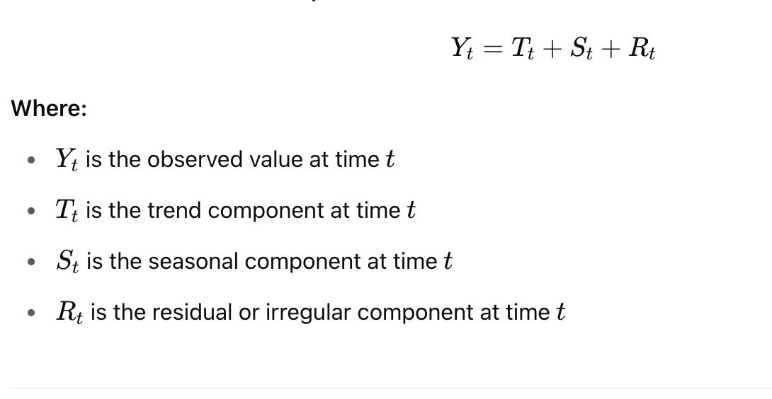
Characteristics: In an additive model, the magnitude of the seasonal fluctuations (and residuals) remains roughly constant over time, regardless of the level of the trend. The seasonal component adds a fixed amount to the trend.
When to Use: This model is appropriate when the variation around the trend does not increase or decrease with the level of the series. For example, if monthly sales vary by approximately +/- $1000$ around the trend, whether the trend is at $10,000$ or $100,000$. This often applies to phenomena where the factors causing seasonality are independent of the magnitude of the series itself (e.g., fixed holiday effects).
Multiplicative Model:
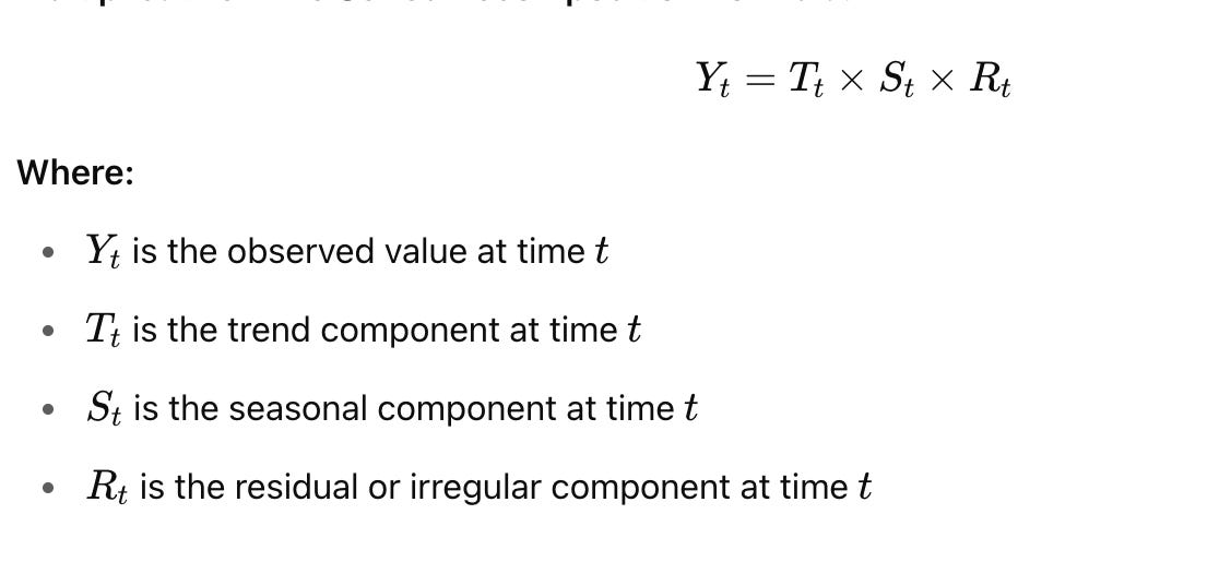
Characteristics: In a multiplicative model, the magnitude of the seasonal fluctuations (and residuals) increases or decreases proportionally with the level of the trend. The seasonal component multiplies the trend.
When to Use: This model is suitable when the amplitude of the seasonal pattern grows or shrinks as the overall level of the series changes. For example, if monthly sales vary by +/- 10% of the trend, meaning the actual dollar variation is much larger when sales are $100,000$ than when they are $10,000$. This is common in economic series like GDP, sales, or population growth, where growth tends to be exponential.
Choosing the Right Model:
Visually inspect the time series plot. If the seasonal fluctuations appear to grow wider or narrower as the series progresses (heteroscedasticity), a multiplicative model is likely more appropriate. If the fluctuations remain relatively constant in width, an additive model is better. If in doubt, try both and compare the clarity of the decomposed components and the characteristics of the residuals. A common trick for multiplicative series is to apply a logarithmic transformation, which can transform a multiplicative relationship into an additive one, allowing the use of additive decomposition methods on the transformed data.
Common Decomposition Algorithms
While the underlying concept is simple, various algorithms are used to perform decomposition:
Moving Averages: A simple and intuitive method where the trend is estimated by smoothing the series using a moving average. Seasonality is then derived by averaging the detrended values for each period.
STL (Seasonal-Trend decomposition using Loess): A more robust and versatile method that uses local regression (LOESS) to estimate the trend and seasonal components. It can handle various types of seasonality and is less sensitive to outliers than traditional moving average methods.
X-11/X-13 ARIMA-SEATS: Sophisticated and widely used methods developed by the U.S. Census Bureau. These are complex seasonal adjustment programs often used for official economic statistics.
Practical Decomposition with Python
Python’s statsmodels library provides powerful tools for time series analysis, including decomposition. We will use seasonal_decompose to illustrate the process.
Setting Up the Environment
First, we need to import the necessary libraries.
import pandas as pd
import numpy as np
import matplotlib.pyplot as plt
from statsmodels.tsa.seasonal import seasonal_decompose
from statsmodels.graphics.tsaplots import plot_acf # For residual analysis
from statsmodels.stats.diagnostic import acorr_ljungbox # For residual analysis
Here, we import pandas for data manipulation, numpy for numerical operations, matplotlib.pyplot for plotting, and seasonal_decompose from statsmodels for the decomposition itself. We also import tools for analyzing residuals later.
Generating a Synthetic Time Series
To clearly understand how decomposition works, let’s create a synthetic time series with known trend, seasonality, and noise components. This allows us to see if the decomposition algorithm can successfully recover these original patterns.
# Define time range for our synthetic data
np.random.seed(42) # For reproducibility
time_index = pd.date_range(start='2010-01-01', periods=120, freq='MS') # 10 years of monthly data
We define a time_index using pd.date_range for 10 years of monthly data, starting from January 2010. freq='MS' specifies month start frequency. np.random.seed(42) ensures our random components are consistent for repeated runs.
# 1. Create a linear trend component
trend = np.linspace(0, 100, len(time_index))
Here, we create a simple linear trend that increases from 0 to 100 over the 120 periods.
# 2. Create a seasonal component (e.g., yearly cycle)
# We'll simulate a strong annual seasonality
month_of_year = time_index.month
seasonal_pattern = np.sin(np.linspace(0, 3 * 2 * np.pi, len(time_index))) * 10
This code generates a sinusoidal seasonal pattern. np.sin creates a wave, and np.linspace ensures it completes 3 cycles over 10 years (3 full cycles per year, 10 years total). Multiplying by 10 sets the amplitude of the seasonality.
# 3. Create a residual (noise) component
noise = np.random.normal(0, 2, len(time_index)) # Mean 0, Std Dev 2
We generate random noise using a normal distribution with a mean of 0 and a standard deviation of 2. This represents the unpredictable part of the series.
Now, let’s combine these components to create our observed time series, first using an additive model.
# Combine components for an ADDITIVE time series
additive_series = pd.Series(trend + seasonal_pattern + noise, index=time_index)
The additive_series is created by simply summing the trend, seasonal, and noise components. We wrap it in a pd.Series with our time_index.
# Combine components for a MULTIPLICATIVE time series
# For multiplicative, ensure components are positive or adjust
trend_mult = np.linspace(10, 100, len(time_index)) # Start trend > 0
seasonal_pattern_mult = 1 + (np.sin(np.linspace(0, 3 * 2 * np.pi, len(time_index))) * 0.2) # Seasonality factor around 1
noise_mult = np.random.normal(1, 0.05, len(time_index)) # Noise factor around 1
multiplicative_series = pd.Series(trend_mult * seasonal_pattern_mult * noise_mult, index=time_index)For a multiplicative series, the components should typically be factors that multiply. Here, seasonal_pattern_mult and noise_mult are constructed to oscillate around 1, so they act as scaling factors. The trend also starts from a positive value.
Finally, let’s visualize our synthetic additive series.
# Plot the synthetic additive time series
plt.figure(figsize=(12, 6))
plt.plot(additive_series, label='Synthetic Additive Series')
plt.title('Synthetic Time Series (Additive Model)')
plt.xlabel('Date')
plt.ylabel('Value')
plt.legend()
plt.grid(True)
plt.show()
This plot displays the combined synthetic series, clearly showing an upward trend with consistent seasonal fluctuations, as expected from an additive model.
Performing Decomposition
We’ll use statsmodels.tsa.seasonal.seasonal_decompose to perform the decomposition. This function takes the time series, the model type ('additive' or 'multiplicative'), and the period of the seasonality as arguments.
# Perform additive decomposition on the synthetic additive series
# period=12 for monthly data with yearly seasonality
result_additive = seasonal_decompose(additive_series, model='additive', period=12)
We apply seasonal_decompose to our additive_series. We explicitly set model='additive' and period=12 because our synthetic data has a clear yearly (12-month) seasonality.
# Plot the decomposed components
plt.figure(figsize=(12, 8))
result_additive.plot()
plt.suptitle('Additive Time Series Decomposition', y=1.02) # Adjust suptitle position
plt.tight_layout(rect=[0, 0, 1, 0.98]) # Adjust layout to prevent title overlap
plt.show()
The plot() method of the decomposition result object conveniently generates subplots for the observed series, trend, seasonal, and residual components. Observe how well the seasonal_decompose function has identified the linear trend and the sinusoidal seasonal pattern that we built into the synthetic data. The residuals should appear as random noise around zero.
Now, let’s try decomposing the multiplicative series we created.
# Perform multiplicative decomposition on the synthetic multiplicative series
result_multiplicative = seasonal_decompose(multiplicative_series, model='multiplicative', period=12)
Here, we use model='multiplicative' as our synthetic series was generated with a multiplicative relationship.
# Plot the decomposed components for the multiplicative series
plt.figure(figsize=(12, 8))
result_multiplicative.plot()
plt.suptitle('Multiplicative Time Series Decomposition', y=1.02)
plt.tight_layout(rect=[0, 0, 1, 0.98])
plt.show()
Again, observe how the decomposition successfully extracts the trend, seasonal, and residual components. Notice how the seasonal component’s amplitude appears to grow with the trend in the original series, which is characteristic of a multiplicative relationship.
Real-World Example: Air Passengers Dataset
Let’s apply decomposition to a classic real-world dataset: monthly international airline passenger numbers from 1949 to 1960. This dataset is famous for exhibiting a clear multiplicative seasonality.
# Load the Air Passengers dataset
# This dataset is often available in seaborn or directly online
# For simplicity, we'll create a dummy one or assume it's loaded as a pandas Series
# In a real scenario, you would load from CSV: pd.read_csv('AirPassengers.csv', index_col='Month', parse_dates=True)
# Dummy Air Passengers data for demonstration (replace with actual load if desired)
data = {
'Month': pd.to_datetime(['1949-01-01', '1949-02-01', '1949-03-01', '1949-04-01', '1949-05-01', '1949-06-01',
'1949-07-01', '1949-08-01', '1949-09-01', '1949-10-01', '1949-11-01', '1949-12-01',
'1950-01-01', '1950-02-01', '1950-03-01', '1950-04-01', '1950-05-01', '1950-06-01',
'1950-07-01', '1950-08-01', '1950-09-01', '1950-10-01', '1950-11-01', '1950-12-01',
'1951-01-01', '1951-02-01', '1951-03-01', '1951-04-01', '1951-05-01', '1951-06-01',
'1951-07-01', '1951-08-01', '1951-09-01', '1951-10-01', '1951-11-01', '1951-12-01',
'1952-01-01', '1952-02-01', '1952-03-01', '1952-04-01', '1952-05-01', '1952-06-01',
'1952-07-01', '1952-08-01', '1952-09-01', '1952-10-01', '1952-11-01', '1952-12-01',
'1953-01-01', '1953-02-01', '1953-03-01', '1953-04-01', '1953-05-01', '1953-06-01',
'1953-07-01', '1953-08-01', '1953-09-01', '1953-10-01', '1953-11-01', '1953-12-01',
'1954-01-01', '1954-02-01', '1954-03-01', '1954-04-01', '1954-05-01', '1954-06-01',
'1954-07-01', '1954-08-01', '1954-09-01', '1954-10-01', '1954-11-01', '1954-12-01',
'1955-01-01', '1955-02-01', '1955-03-01', '1955-04-01', '1955-05-01', '1955-06-01',
'1955-07-01', '1955-08-01', '1955-09-01', '1955-10-01', '1955-11-01', '1955-12-01',
'1956-01-01', '1956-02-01', '1956-03-01', '1956-04-01', '1956-05-01', '1956-06-01',
'1956-07-01', '1956-08-01', '1956-09-01', '1956-10-01', '1956-11-01', '1956-12-01',
'1957-01-01', '1957-02-01', '1957-03-01', '1957-04-01', '1957-05-01', '1957-06-01',
'1957-07-01', '1957-08-01', '1957-09-01', '1957-10-01', '1957-11-01', '1957-12-01',
'1958-01-01', '1958-02-01', '1958-03-01', '1958-04-01', '1958-05-01', '1958-06-01',
'1958-07-01', '1958-08-01', '1958-09-01', '1958-10-01', '1958-11-01', '1958-12-01',
'1959-01-01', '1959-02-01', '1959-03-01', '1959-04-01', '1959-05-01', '1959-06-01',
'1959-07-01', '1959-08-01', '1959-09-01', '1959-10-01', '1959-11-01', '1959-12-01',
'1960-01-01', '1960-02-01', '1960-03-01', '1960-04-01', '1960-05-01', '1960-06-01',
'1960-07-01', '1960-08-01', '1960-09-01', '1960-10-01', '1960-11-01', '1960-12-01']),
'Passengers': [112, 118, 132, 129, 121, 135, 148, 148, 136, 119, 104, 118,
115, 126, 141, 135, 125, 149, 170, 170, 158, 133, 114, 140,
145, 150, 178, 163, 172, 178, 199, 199, 184, 162, 146, 166,
171, 180, 193, 181, 183, 218, 230, 242, 209, 191, 172, 194,
196, 196, 236, 235, 229, 243, 264, 272, 237, 211, 180, 201,
204, 188, 235, 227, 234, 264, 302, 293, 259, 229, 203, 229,
242, 233, 267, 269, 270, 315, 364, 347, 312, 274, 237, 278,
284, 277, 317, 313, 318, 374, 413, 405, 355, 306, 271, 306,
337, 305, 356, 346, 346, 412, 472, 461, 390, 342, 301, 335,
340, 318, 362, 348, 363, 435, 491, 505, 404, 359, 310, 337,
360, 342, 406, 396, 420, 472, 548, 559, 463, 407, 362, 405,
417, 391, 419, 461, 472, 535, 622, 606, 508, 461, 390, 432]
}
air_passengers = pd.Series(data['Passengers'], index=data['Month'])This block provides a hardcoded version of the Air Passengers dataset for immediate use. In a real-world scenario, you’d typically load this from a .csv file.
# Plot the original Air Passengers series
plt.figure(figsize=(12, 6))
plt.plot(air_passengers, label='Air Passengers')
plt.title('Monthly International Air Passengers (1949-1960)')
plt.xlabel('Date')
plt.ylabel('Passengers')
plt.legend()
plt.grid(True)
plt.show()
The plot clearly shows an upward trend and seasonal fluctuations that increase in amplitude over time, indicating a multiplicative relationship.
# Perform multiplicative decomposition on the Air Passengers series
# period=12 for monthly data with yearly seasonality
result_air_passengers = seasonal_decompose(air_passengers, model='multiplicative', period=12)
Based on the visual inspection, we choose the multiplicative model for this dataset.
# Plot the decomposed components for Air Passengers
plt.figure(figsize=(12, 8))
result_air_passengers.plot()
plt.suptitle('Air Passengers Time Series Decomposition (Multiplicative)', y=1.02)
plt.tight_layout(rect=[0, 0, 1, 0.98])
plt.show()
The decomposition beautifully separates the clear upward trend, the consistent annual seasonality, and the remaining residuals. Notice how the seasonal component is now a factor (around 1), and its pattern is stable, while its effect on the original series grows due to multiplication with the increasing trend.
Analyzing Residuals
The residual component is often overlooked but is crucial for assessing the quality of the decomposition and for subsequent forecasting model development. Ideally, the residuals should be white noise — random, uncorrelated, and with a constant variance.
The Role of Residuals
Unexplained Variance: Residuals represent the part of the series that cannot be attributed to the identified trend or seasonal patterns.
Model Fit Indicator: If your decomposition (or a subsequent forecasting model) is a good fit for the data, the residuals should contain no discernible patterns. Any remaining pattern suggests that the decomposition (or model) has not fully captured all the underlying structure.
Anomaly Detection: Outliers or unusual events in the original series will often manifest as large spikes in the residual component, making them easier to spot.
Checking for White Noise
We can visually inspect and statistically test the residuals for white noise characteristics.
# Plot the residuals from the Air Passengers decomposition
plt.figure(figsize=(12, 4))
plt.plot(result_air_passengers.resid)
plt.title('Residuals from Air Passengers Decomposition')
plt.xlabel('Date')
plt.ylabel('Residual Value')
plt.grid(True)
plt.show()
Visually, the residuals from the Air Passengers decomposition appear somewhat random, but there might be some small variations in variance.
# Plot the Autocorrelation Function (ACF) of the residuals
# This helps identify if there's any remaining correlation (pattern) in the residuals
plt.figure(figsize=(12, 5))
plot_acf(result_air_passengers.resid.dropna(), lags=40, ax=plt.gca()) # dropna() handles NaNs at ends
plt.title('Autocorrelation Function of Residuals')
plt.xlabel('Lag')
plt.ylabel('Autocorrelation')
plt.show()
The Autocorrelation Function (ACF) plot shows the correlation of a time series with its own past values (lags). For white noise, all autocorrelations (except at lag 0, which is always 1) should be close to zero and fall within the confidence bands (the blue shaded area). If significant spikes are outside these bands, it suggests remaining correlation, meaning the residuals are not pure white noise and there’s uncaptured information. In the Air Passengers example, the ACF generally falls within the bands, suggesting the residuals are largely random.
# Perform the Ljung-Box test on the residuals
# This is a statistical test for white noise
# It tests the null hypothesis that there is no autocorrelation up to a specified lag.
# A high p-value (e.g., > 0.05) suggests that the residuals are independently distributed (white noise).
ljungbox_test_results = acorr_ljungbox(result_air_passengers.resid.dropna(), lags=[10, 20], return_df=True)
print(ljungbox_test_results)
The Ljung-Box test is a formal statistical test for autocorrelation in the residuals. The null hypothesis ($H_0$) is that the data are independently distributed (i.e., residuals are white noise). If the p-value is greater than a chosen significance level (commonly 0.05), we fail to reject the null hypothesis, suggesting the residuals are indeed white noise. We test at multiple lags (e.g., 10 and 20) to check for short and longer-term dependencies. For the Air Passengers residuals, if the p-values are high, it supports the notion that the decomposition has effectively isolated the trend and seasonality.
Practical Implications of Residuals
Model Validation: Thorough analysis of residuals is a critical step in validating any time series model. If residuals show patterns, it indicates that your model is inadequate and needs refinement.
Feature Engineering: If residuals are not white noise, the patterns within them might suggest new features to incorporate into a more complex forecasting model (e.g., adding a new predictor variable, or using a more sophisticated model that can capture higher-order dependencies).
Anomaly Detection: Monitoring residuals over time is an effective way to detect sudden, unexpected changes in the underlying process, which could signal system failures, unusual market events, or data errors.
Impact on Forecasting Model Selection
Understanding the components of a time series directly informs the choice and complexity of forecasting models:
Trend: If a strong trend is present, models that can explicitly capture and extrapolate trends (e.g., ARIMA models with differencing, Exponential Smoothing methods like Holt’s or Holt-Winters, or regression models with time as a predictor) are appropriate.
Seasonality: For series with clear seasonality, models that explicitly account for seasonal patterns are necessary. This includes Seasonal ARIMA (SARIMA), Seasonal Exponential Smoothing (Holt-Winters), or models like Prophet that explicitly model seasonal effects.
Stationarity: Decomposing a series can help achieve stationarity (constant mean, variance, and autocorrelation over time), which is a key assumption for many traditional forecasting models like ARIMA. By removing trend and seasonality, the remaining residuals are often closer to a stationary process.
Feature Engineering: The seasonal component can be extracted and used to create new features for machine learning models (e.g., creating dummy variables for months or days of the week, or sine/cosine transformations to capture cyclical patterns). The trend component can also be used as a feature or modeled separately.
By systematically breaking down a time series into its fundamental components, we gain profound insights into its behavior, which is an indispensable step towards accurate analysis and reliable forecasting.
The Comprehensive Time Series Forecasting Project Roadmap
Developing accurate and actionable time series forecasts involves far more than simply running a statistical model. It’s a comprehensive, cyclical process that bridges business objectives with technical execution, requiring collaboration across various roles. A structured approach, often referred to as a “forecasting project roadmap” or “lifecycle,” is essential for success. This roadmap ensures that forecasting efforts are aligned with strategic goals, data quality is maintained, models are robust, and their outputs are effectively utilized and continuously improved. Neglecting any stage can lead to models that are technically sound but fail to deliver real-world value or quickly become obsolete.
Let’s explore the key stages of a typical time series forecasting project.
Define the Business Problem and Goals
This initial stage is arguably the most critical yet often overlooked. Before collecting any data or thinking about models, it’s paramount to clearly articulate why a forecast is needed and what specific business decision it will inform.
Why it’s Crucial:
Clarity and Direction: A well-defined problem provides a clear objective for the entire project, preventing aimless data exploration or model building.
Alignment with Business Value: It ensures the forecasting effort directly contributes to an organizational goal, such as cost reduction, revenue increase, or improved efficiency.
Defines Success Metrics: Understanding the business problem helps identify the key performance indicators (KPIs) that will measure the forecast’s success. For instance, is accuracy paramount, or is it more important to avoid stockouts?
Scope Definition: Helps to bound the problem, preventing “scope creep” where the project expands beyond its original intent.
Key Activities:
Stakeholder Interviews: Engage with business users, domain experts, and decision-makers to understand their needs, current challenges, and desired outcomes.
Problem Framing: Translate vague business questions into specific, measurable forecasting problems (e.g., “predict next month’s sales for product X,” “forecast hourly energy demand for the next 24 hours”).
KPI Identification: Define the metrics that will quantify the impact and success of the forecast (e.g.,
Mean Absolute Error (MAE),Root Mean Squared Error (RMSE),forecast bias,inventory turnover rate).Time Horizon and Granularity: Determine the required forecasting horizon (e.g., next day, next month, next year) and the granularity (e.g., hourly, daily, weekly, monthly).
Common Pitfalls:
Vague Objectives: Starting with “we need a forecast” without specifying for what purpose or how it will be used.
Lack of Business Context: Developing a technically accurate model that doesn’t solve the actual business problem or isn’t actionable.
Ignoring Stakeholders: Building a solution in isolation without input from those who will use it.
Typical Roles Involved: Business Analyst, Product Manager, Domain Expert, Lead Data Scientist.
Example: Camping Trip Scenario
Imagine you’re planning a multi-day camping trip and want to choose the right sleeping bag.
Business Problem: Select a sleeping bag that will keep me comfortable, but not overheated, given the expected overnight temperatures.
Goal: Forecast the minimum overnight temperature for each night of the trip to inform sleeping bag selection.
Success Metric: My comfort level (subjective, but we can aim for the sleeping bag’s comfort rating to match the forecast temperature).
Time Horizon/Granularity: Daily minimum temperature for the next 3–5 days.
Example: Retail Sales Forecasting
A retail chain wants to optimize inventory and staffing
Business Problem: Accurately predict future sales to minimize stockouts, reduce excess inventory holding costs, and optimize staffing levels in stores.
Goal: Forecast daily sales for each product SKU at each store location for the next 4–6 weeks.
Success Metrics:
MAPE(Mean Absolute Percentage Error) for sales,stockout rate,inventory turnover.Time Horizon/Granularity: Daily sales forecasts for individual SKUs at specific store locations, looking 4–6 weeks ahead.
Gather and Prepare Data
Once the problem is clear, the next crucial step is to acquire and ready the data that will fuel your forecasting model. Data quality directly impacts model performance; “garbage in, garbage out” is particularly true in time series forecasting.
Why it’s Crucial:
Data as Fuel: High-quality, relevant historical data is the fundamental input for any time series model.
Reliability: Clean and well-prepared data ensures that the patterns identified by the model are genuine and not artifacts of data errors or inconsistencies.
Feature Engineering Foundation: This stage lays the groundwork for creating meaningful features that capture underlying drivers of the time series.
Key Activities:
Data Source Identification: Locate all relevant data sources (e.g., internal databases, APIs, external datasets). This might include the target time series itself (e.g., sales, temperature) and potential exogenous variables (e.g., promotions, holidays, economic indicators).
Data Extraction (ETL/ELT): Retrieve data from various sources. This can involve writing scripts to connect to databases, consume APIs, or parse files.
Data Cleaning: Address common data issues:
Missing Values: Impute (e.g., interpolation, mean/median) or remove missing data points.
Outliers: Identify and handle extreme values that might distort patterns (e.g., capping, removal, or specialized robust methods).
Inconsistent Formats: Standardize data types, date formats, and categorical encodings.
Duplicates: Remove redundant entries.
Data Transformation: Reshape data for analysis, aggregate to the desired granularity (e.g., from hourly to daily), or normalize/standardize numerical features.
Preliminary Feature Engineering (Conceptual): At this stage, you might start thinking about and creating basic features like
lagged values(past observations),moving averages, ortime-based features(day of week, month, year).Common Pitfalls:
Data Silos: Relevant data being scattered across different departments or systems, making it hard to access.
Poor Data Quality: Assuming data is clean, leading to models built on flawed information.
Insufficient Historical Data: Time series models often require a significant amount of historical data to identify trends and seasonality reliably.
Data Leakage: Accidentally including future information in the training data, leading to overly optimistic evaluation results.
Typical Roles Involved: Data Engineer, Data Scientist.
Example: Camping Trip Scenario
Data Collection: Access historical weather data for the camping location (temperature, precipitation, wind speed), potentially from weather APIs or historical records. Also, gather personal notes from past trips (e.g., “felt cold with 40F sleeping bag at 35F”).
Data Preparation: Clean weather data (handle missing temperature readings), align dates, and perhaps average temperatures over the night.
Example: Retail Sales Forecasting
Data Collection: Extract historical sales transaction data (SKU, quantity, price, date, store ID), promotional calendars, holiday schedules, and possibly external economic indicators (e.g., consumer confidence index, local unemployment rates).
Data Preparation: Aggregate transactional data to daily SKU-store sales. Identify and handle missing sales records. Clean up inconsistent product IDs. Create features like
is_promotion,day_of_week,is_holiday.
Develop a Forecasting Model
This is where the core predictive engine is built. It involves selecting, training, and optimizing a model based on the prepared historical data.
Why it’s Crucial: This stage translates the patterns and relationships identified in the data into a predictive algorithm that can generate future forecasts.
Key Activities (High-Level Conceptual):
Data Splitting: Divide the historical data into
training,validation(ordevelopment), andtestsets. For time series, this is typically done chronologically (pastfor training,futurefor validation/test) to simulate real-world forecasting.Feature Engineering (Advanced): Beyond basic time-based features, this might involve creating more complex interactions, polynomial features, or transformations specific to the chosen model.
Model Selection: Choose appropriate forecasting algorithms. This could range from traditional statistical models (e.g.,
ARIMA,Exponential Smoothing,Prophet) to machine learning models (e.g.,Random Forest,XGBoost,LightGBM) or deep learning models (e.g.,LSTMs,Transformers) depending on data complexity, volume, and required interpretability.Model Training: Fit the selected model(s) to the training data. This process learns the underlying patterns and relationships between features and the target variable.
Hyperparameter Tuning: Optimize the model’s internal parameters (hyperparameters) using the validation set to achieve the best performance without overfitting. This might involve techniques like
grid search,random search, orBayesian optimization.
Common Pitfalls:
Overfitting/Underfitting: Building a model that performs perfectly on training data but poorly on new data (overfitting), or a model that is too simplistic and doesn’t capture underlying patterns (underfitting).
Ignoring Baseline Models: Not comparing complex models against simple baselines (e.g.,
naive forecast,seasonal naive) to ensure added complexity is justified.Lack of Interpretability: Choosing a “black box” model when explainability is crucial for business trust and decision-making.
Typical Roles Involved: Data Scientist, Machine Learning Engineer.
Example: Camping Trip Scenario
Model Selection: A simple rule-based model: “If the forecast minimum temperature is below 30F, use a 0F bag; if between 30–45F, use a 30F bag; otherwise, use a light bag.” Or a basic linear regression using historical temperature data.
Training: If using regression, train the model on past temperature vs. comfort data.
Example: Retail Sales Forecasting
Model Selection: Experiment with various models like
Prophet(for strong seasonality and holidays),ARIMA(for autocorrelation), orXGBoost(for incorporating many exogenous variables like promotions). For large-scale forecasting across many SKUs, a hierarchical approach or a deep learning model might be considered.Training: Train the chosen model(s) on historical sales data, incorporating features like
day_of_week,month,promotional flags, andlagged sales.
Evaluate and Validate the Model
After developing a model, it’s critical to rigorously evaluate its performance using unseen data to ensure its reliability and generalization capabilities. This step is about confirming that the model will perform well in the real world.
Why it’s Crucial:
Trust and Reliability: Provides confidence that the model’s predictions are accurate and trustworthy.
Preventing Over-Optimism: Evaluation on a separate test set prevents overestimating performance due to overfitting on training data.
Informing Deployment: A well-validated model is a prerequisite for successful deployment.
Error Analysis: Helps understand where and why the model makes mistakes, guiding further improvements.
Key Activities:
Defining Evaluation Metrics: Choose appropriate metrics based on the business problem (e.g.,
MAE,RMSE,MAPE,sMAPE,R-squared,directional accuracy). Some metrics are better for specific error types or business contexts.Backtesting/Out-of-Sample Validation: Evaluate the model’s performance on the
test set(data the model has never seen), mimicking how it would perform on future data. For time series, this often involves "rolling forecast origin" or "walk-forward validation" where the model is retrained and evaluated on successive time windows.Sensitivity Analysis: Understand how robust the model is to changes in input data or assumptions.
Error Analysis: Investigate patterns in prediction errors. Are errors higher on weekends? During promotions? For certain product categories? This provides insights for model refinement.
Business Impact Assessment: Translate statistical accuracy into business implications (e.g., “a 5%
MAPEmeans we might overstock by X units or understock by Y units, costing Z dollars").
Common Pitfalls:
Using Inappropriate Metrics: Choosing metrics that don’t align with the business goal (e.g., using
RMSEwhenMAPEis more relevant for percentage errors).Evaluating on Training Data Only: Leading to an inflated sense of accuracy.
Ignoring Business Context of Errors: Not understanding the real-world cost or impact of different types of forecasting errors.
Typical Roles Involved: Data Scientist, Business Analyst.
Example: Camping Trip Scenario
Evaluation: After the trip, compare the forecast minimum temperatures against the actual minimum temperatures recorded. Did the sleeping bag recommendation align with your comfort level? If not, why? (e.g., wind chill wasn’t factored in).
Metrics: A simple count of “comfortable” vs. “uncomfortable” nights.
Example: Retail Sales Forecasting
Evaluation: Compare the model’s daily SKU-store sales forecasts against actual sales data for the test period.
Metrics: Calculate
MAPEandRMSEfor different product categories, stores, and time periods. Analyzeforecast bias(is the model consistently over- or under-forecasting?). Present these metrics to stakeholders in an understandable way.
Deploy to Production
Once a model has been thoroughly validated and deemed fit for purpose, it needs to be integrated into the operational environment so that its forecasts can be used for real-world decision-making.
Why it’s Crucial:
Actionable Insights: Deployment makes the forecast accessible to business users and systems, allowing them to act on the predictions.
Automation: Automates the forecasting process, reducing manual effort and ensuring timely availability of predictions.
Scalability: Enables the model to generate forecasts at the required scale and frequency.
Key Activities:
Model Serialization: Save the trained model in a deployable format (e.g.,
picklefile,ONNX,PMML).API Development: Wrap the model in an API (e.g.,
REST APIusing Flask or FastAPI) so other applications can easily request forecasts.Integration with Existing Systems: Connect the forecasting service with business applications (e.g., inventory management systems, ERPs, dashboards). This might involve setting up data pipelines to feed inputs to the model and consume its outputs.
Infrastructure Provisioning: Set up the necessary computing resources (e.g., cloud instances, containers like Docker, orchestration with Kubernetes) to host the model.
Automated Pipelines: Establish
CI/CD(Continuous Integration/Continuous Deployment) pipelines for model updates and automated retraining.Common Pitfalls:
Lack of MLOps Maturity: Underestimating the complexity of operationalizing machine learning models compared to traditional software.
Integration Complexities: Difficulty connecting the model with legacy systems.
Scalability Issues: The deployed model cannot handle the required volume of predictions or concurrent requests.
Security Concerns: Neglecting data security and access control for the deployed model.
Typical Roles Involved: MLOps Engineer, Software Engineer, Data Scientist.
Example: Camping Trip Scenario
Deployment: Create a simple script or web application that takes the trip dates and location as input, queries a weather API for forecast temperatures, and then applies your sleeping bag rule to recommend a bag. Share this tool with friends.
Example: Retail Sales Forecasting
Deployment: The forecasting model is packaged into a container (e.g., Docker image) and deployed on a cloud platform (e.g., AWS SageMaker, Azure ML, Google Cloud AI Platform). An API endpoint is exposed that inventory management systems can call daily to get updated sales forecasts for all SKUs and stores. An automated data pipeline ensures the model receives fresh input data regularly.
Monitor and Maintain
Deployment is not the end of the project; it’s the beginning of its operational life. Models, especially those relying on time-dependent data, can degrade over time due to changes in underlying patterns. Continuous monitoring and maintenance are crucial.
Why it’s Crucial:
Sustained Performance: Ensures the model continues to provide accurate and relevant forecasts over time.
Detecting Degradation: Identifies “model drift” or “concept drift” where the relationship between input features and the target variable changes.
Addressing Data Quality Issues: Catches problems in the data pipeline that could impact model inputs.
Business Relevance: Ensures the model adapts to evolving business conditions and goals.
Key Activities:
Performance Monitoring: Continuously track model performance metrics (e.g.,
MAE,MAPE,bias) against actual outcomes. Set up dashboards and alerts for significant deviations.Data Quality Monitoring: Monitor the incoming data pipeline for anomalies, missing values, or changes in data distribution that could affect the model.
Concept Drift Detection: Implement mechanisms to detect when the underlying patterns the model learned are no longer valid (e.g., due to market shifts, new products, policy changes).
Retraining Schedules: Establish a regular schedule for retraining the model with new historical data to keep it updated.
A/B Testing: Experiment with new model versions or features by deploying them alongside the existing model to evaluate real-world performance before full rollout.
Model Versioning: Maintain versions of models and their associated code/data for reproducibility and rollback capabilities.
Common Pitfalls:
Stale Models: Deploying a model and never revisiting it, leading to rapidly degrading performance.
Ignoring Data Pipeline Issues: Assuming data quality will remain constant.
Lack of Alert Systems: Not being notified when model performance degrades or data issues arise.
No Feedback Loop: Not collecting feedback from business users on the usefulness or accuracy of the forecasts.
Typical Roles Involved: MLOps Engineer, Data Scientist, Operations Team.
Example: Camping Trip Scenario
Monitoring: After each trip, review how well the sleeping bag recommendation performed. Did you consistently feel too cold or too hot?
Maintenance: If you consistently feel cold, perhaps update your rule to be more conservative or incorporate additional factors like wind.
Example: Retail Sales Forecasting
Monitoring: Set up automated dashboards that track daily
MAPEandbiasfor sales forecasts across different stores and product categories. Configure alerts to notify the data science team ifMAPEexceeds a certain threshold or if significantbiasis detected.Maintenance: Schedule monthly retraining of the model with the latest sales data. If a new major promotional strategy is introduced, the model might need a significant update or even redevelopment to incorporate these new dynamics.
Setting a Goal
Before embarking on any time series forecasting endeavor, the single most crucial step is to define a clear, actionable goal. This initial phase, often overlooked in the rush to gather data and apply algorithms, determines the ultimate success and relevance of your entire forecasting project. Without a well-articulated goal, your efforts risk becoming aimless, producing forecasts that, while technically sound, provide no real value or actionable insights.
The Foundation: Why a Clear Goal is Paramount
Think of a forecasting project as a journey. Your goal is the destination. Without knowing where you’re going, any path you take will be arbitrary, and you might end up somewhere completely unhelpful. In the context of time series forecasting, defining your goal means answering the fundamental question: What decision will this forecast help me make, or what problem will it help me solve?
This seemingly simple question is the bedrock upon which all subsequent steps are built. It dictates:
What specific variable needs to be forecast.
The required accuracy and precision of the forecast.
The time horizon of the forecast (e.g., next day, next month, next year).
The resources (data, tools, personnel) you’ll need.
How the forecast will be evaluated for success.
Characteristics of a “Good” Forecasting Goal
A robust forecasting goal isn’t just a vague aspiration; it possesses specific characteristics that make it effective and actionable. While not strictly adhering to the full SMART (Specific, Measurable, Achievable, Relevant, Time-bound) criteria often used in project management, we can adapt its essence to forecasting:
Specific: The goal must clearly state what needs to be achieved. Instead of “forecast sales,” a specific goal might be “forecast daily sales of product X for the next month.”
Actionable: The forecast derived from the goal must directly lead to a decision or an action. If the forecast doesn’t inform a concrete step, its utility is limited. For example, “forecast future temperature to decide which sleeping bag to pack” is actionable.
Measurable: You must be able to quantify whether the goal has been met. This often relates to the impact of the forecast. For instance, “reduce inventory holding costs by 10% by optimizing stock levels based on demand forecasts.”
Relevant: The goal must align with broader organizational objectives or personal needs. Forecasting for the sake of forecasting is rarely beneficial. It should address a genuine problem or opportunity.
Time-bound (Implied by Horizon): While the goal itself might not always have an explicit deadline, the forecast it requires will always have a defined time horizon (e.g., “forecast for the next quarter,” “predict next week’s demand”). This implicitly makes the goal time-bound in terms of its utility.
The Perils of a Vague Goal
Failing to define a clear goal is one of the most common pitfalls in any data science or forecasting project. A vague or ill-defined goal can lead to:
Irrelevant Forecasts: You might accurately forecast something, but if it doesn’t align with a decision or problem, the forecast is useless. Imagine forecasting the price of a stock when your actual goal was to predict overall market sentiment.
Wasted Effort and Resources: Without a clear target, teams can spend significant time and money collecting irrelevant data, developing complex models that don’t address the core need, or chasing elusive metrics.
Scope Creep: The project can endlessly expand as new, loosely related questions arise, derailing progress and delaying completion.
Difficulty in Evaluation: If you don’t know what success looks like from the outset, it’s impossible to objectively evaluate the performance and value of your forecasting model.
Project Failure: Ultimately, a lack of direction can lead to projects being abandoned or failing to deliver any meaningful impact.
How the Goal Shapes the Forecast Type
Your defined goal directly influences the type of forecast you need to produce. Different goals require different outputs:
Point Forecast vs. Probabilistic Forecast:
If your goal is to know the most likely single value (e.g., “What will be the exact temperature tomorrow?”), you need a point forecast.
If your goal involves understanding uncertainty and risk (e.g., “What is the probability that the temperature will drop below freezing tomorrow?” or “What range of temperatures is most likely?”), you need a probabilistic forecast (e.g., prediction intervals or full probability distributions). This is crucial for risk management or setting safety stock levels.
Short-Term vs. Long-Term Forecast:
A goal like “optimize staffing for tomorrow’s call center volume” requires a short-term forecast (hourly, daily).
A goal like “plan capital expenditure for new factory capacity over the next five years” requires a long-term forecast (yearly). The methods and data used for these will differ significantly.
Univariate vs. Multivariate Forecast:
If your goal is simply “predict the future value of a single variable” (e.g., “How much electricity will be consumed next hour?”), you might need a univariate forecast.
If your goal requires understanding the relationship and future values of multiple interdependent variables (e.g., “Predict sales of product A and product B simultaneously, considering their cross-promotions”), you might need a multivariate forecast.
Real-World Applications: From Personal Decisions to Business Strategy
Let’s solidify the connection between goal and forecast with examples.
Personal Scenario: The Camping Trip
Imagine your goal is to sleep comfortably on your camping trip next weekend. This is a clear, actionable personal goal. To achieve this, you need to make a decision about what kind of sleeping bag to pack. This decision, in turn, depends on anticipating the conditions.
Goal: Sleep comfortably on the camping trip.
Decision Informed by Forecast: Which sleeping bag (and other gear) to pack.
Need for Forecast: To make the right decision, you need to know the anticipated overnight temperature. Therefore, you need a temperature forecast.
Type of Forecast: A point forecast of the minimum overnight temperature, perhaps with a range (probabilistic forecast) to account for uncertainty, for the specific location and dates of your trip.
Impact: Packing the right gear ensures comfort and safety, achieving the goal.
This simple example illustrates how a personal comfort goal directly translates into the need for a specific type of forecast.
Business Scenario: Retail Inventory Optimization
Now, let’s consider a business context. A large retail company faces challenges with inventory: either too much stock leading to high holding costs and waste, or too little stock leading to lost sales and customer dissatisfaction.
Goal:
Optimize inventory levels to minimize holding costs while ensuring product availability for customers. This is a specific, measurable, and relevant business goal.Decision Informed by Forecast: How much of each product to order from suppliers, and when.
Need for Forecast: To make informed ordering decisions, the company needs to anticipate future customer demand for each product. Therefore, they need a product demand forecast.
Type of Forecast: This would likely involve thousands of individual point forecasts (e.g., daily sales units per SKU) for a short to medium-term horizon (e.g., next 1–3 months), potentially with probabilistic forecasts (prediction intervals) to manage stockout risk. It might also involve multivariate forecasts if demand for certain products is interdependent or influenced by shared factors like promotions.
Impact: Accurate demand forecasts enable the company to order just enough stock, reducing excess inventory costs, minimizing waste, and preventing lost sales due to stockouts, directly contributing to the goal and improving profitability.
In both examples, the initial goal-setting phase is paramount. It serves as the guiding star, ensuring that all subsequent data collection, model development, and evaluation efforts are aligned with delivering tangible value and solving a real-world problem. This foundational step is what transforms raw data and complex algorithms into actionable intelligence.
Determining What Must Be Forecast to Achieve Your Goal
After establishing a clear and actionable goal for your forecasting project, the next critical step is to translate that high-level objective into a precise, quantifiable variable that needs to be predicted. This step acts as the crucial bridge between an abstract business need and the concrete data science task. It dictates what data you will collect, what models you might use, and ultimately, how you will measure the success of your forecast.
The Translation Process: From Goal to Forecast Target
Defining what must be forecast involves a process of decomposition and specificity. You start with your overarching goal and then ask: “What specific, measurable future value or event, if known, would directly enable me to achieve this goal?”
Consider the following thought process:
Analyze the Goal: Revisit your goal and identify the core uncertainty that prevents you from achieving it.
Identify the Unknown: Pinpoint the specific piece of information that, if you had it for the future, would resolve that uncertainty.
Quantify the Unknown: Can this unknown be expressed as a number, a category, or a specific value? If not, how can it be made measurable?
Define Granularity and Horizon: Over what time period (e.g., hourly, daily, weekly, monthly) and how far into the future (e.g., next hour, next quarter) do you need this forecast?
This step is paramount because it ensures that your efforts in data collection, model development, and analysis are focused and aligned with the project’s ultimate purpose. Without a clearly defined forecast target, you risk collecting irrelevant data, building models that don’t address the core problem, or failing to deliver a valuable solution.
Impact on Downstream Project Phases
The variable you choose to forecast has far-reaching implications across your entire forecasting project roadmap:
Data Collection: The forecast target directly determines what historical data you need to gather. If you decide to forecast
daily sales, you will need historical records ofdaily sales. If you switch toweekly sales, your data aggregation strategy changes. Similarly, potential exogenous variables (features that might influence your target) are also guided by the nature of the target variable.Feature Engineering: The characteristics of your forecast target influence the types of features you might engineer. For example, if forecasting
customer churn, features related to customer interaction frequency, service usage, or past complaints become highly relevant.Model Selection: The nature of the variable (continuous, categorical, count data) will guide your choice of forecasting models. Forecasting a continuous variable like
temperaturemight lead you to regression models, while forecastingnumber of support tickets(count data) might suggest Poisson regression or specific time series models for count data.Evaluation Metrics: How you measure the accuracy and utility of your forecast is entirely dependent on what you are forecasting. For
continuous variables, metrics like Mean Absolute Error (MAE) or Root Mean Squared Error (RMSE) are common. Forclassification tasks(e.g., predicting if a customer will churn), metrics like accuracy, precision, or recall would be used.
Real-World Examples of Defining Forecast Targets
Let’s explore several practical scenarios to solidify your understanding of this crucial translation process:
Example 1: The Comfortable Camping Trip
High-Level Goal: Have a comfortable and enjoyable camping trip this weekend.
Core Uncertainty: What weather conditions will be present, especially overnight?
What Must Be Forecast?
To be comfortable, you need to pack appropriate sleeping gear. The most critical factor for sleeping comfort is typically the
minimum overnight temperature.While
rainfallis also important, for "comfort" related to warmth,minimum temperatureis the direct driver for packing decisions (e.g., sleeping bag rating, extra blankets).Forecast Target:
Minimum overnight temperature (in degrees Celsius/Fahrenheit)for the specific location and dates of the trip.Implication: You would seek historical temperature data, and potentially other weather variables like humidity or wind chill, to build a model that predicts this specific temperature.
Example 2: Inventory Management and Stockouts
High-Level Goal: Reduce stockouts for Product X at our main distribution center, ensuring product availability for customers.
Core Uncertainty: How much of Product X will customers buy or demand in the coming period?
What Must Be Forecast?
To prevent stockouts, you need to know how much product to have on hand. This directly relates to
customer demand.The granularity matters:
daily demand,weekly demand, ormonthly demandfor Product X, depending on lead times and ordering frequency.Forecast Target:
Daily/weekly/monthly demand (in units)for Product X.Implication: Your model would consume historical sales data for Product X, potentially incorporating factors like promotions, seasonality, or competitor actions, to predict future demand. This forecast then directly informs purchasing and inventory replenishment decisions.
Example 3: Optimizing Customer Support Staffing
High-Level Goal: Optimize staffing levels for the customer support team to minimize customer wait times while controlling operational costs.
Core Uncertainty: How many customer inquiries will arrive at any given time?
What Must Be Forecast?
To staff appropriately, you need to anticipate the incoming workload. This workload is best represented by the
number of incoming support ticketsorcalls.The granularity here is often quite fine-grained, such as
number of incoming support tickets per houror evenper 15-minute interval, to allow for dynamic staffing adjustments.Forecast Target:
Number of incoming support tickets/calls (count)per hour/interval.Implication: Your model would analyze historical ticket volumes, considering factors like time of day, day of week, marketing campaigns, or product launches, to predict future call/ticket volumes. This forecast directly guides workforce management systems for scheduling agents.
Addressing Complexities and Pitfalls
While the concept of identifying a single forecast target seems straightforward, real-world scenarios can present challenges:
Multiple Forecast Targets for a Single Goal: Sometimes, a single overarching goal requires forecasts of multiple interdependent variables. For instance, optimizing a complex supply chain might require forecasting
customer demand,supplier lead times, andtransportation costssimultaneously. In such cases, each of these becomes a distinct forecasting task, potentially leading to multiple models or a multi-output model.Non-Obvious Targets or Proxy Variables: The most direct variable might not always be the easiest or even possible to forecast directly. You might need to forecast a proxy variable that correlates strongly with your actual interest. For example, if you want to forecast
customer satisfaction(which is hard to quantify directly and immediately), you might instead forecastcustomer service interaction ratingsorproduct return ratesas proxies.Avoiding “Forecasting Everything”: A common pitfall is to try and forecast too many things, or to forecast a variable that is only tangentially related to the goal. This leads to wasted effort, diluted focus, and models that don’t provide clear business value. Always return to the question: “What must I know to achieve this specific goal?”
Best Practices for Target Identification
Be Specific and Quantifiable: Ensure the variable is measurable and has clear units (e.g., “units sold,” “degrees Celsius,” “number of calls”). Avoid vague terms.
Align with Business Action: The forecast should directly inform a decision or action. If knowing the forecast doesn’t change what you do, it might not be the right target.
Consider Granularity and Horizon: Define the time scale (hourly, daily, weekly) and the forecast horizon (how far into the future) that are most relevant to the decision-making process. Forecasting
monthly salesis useless if you need to optimizedaily staffing.Iterate if Necessary: It’s possible that after some initial data exploration or model building, you realize your chosen forecast target isn’t quite right. Be prepared to revisit and refine it based on new insights.
By meticulously defining what needs to be forecast, you lay a solid foundation for the subsequent steps in your forecasting project, ensuring that your efforts are efficient, relevant, and ultimately successful.
Setting the Horizon of the Forecast
The previous steps established the overarching goal of your forecasting project and precisely identified the specific variable to be predicted. The next critical step is to define the forecast horizon. This term refers to the specific future period for which you need predictions. It’s not merely a duration; it encompasses both the start time and the duration of the forecast period.
What is the Forecast Horizon?
Formally, the forecast horizon is the future time interval for which a time series model will generate predictions. It is defined by two key components:
Forecast Start Time: This is the precise point in time immediately following the last known observation of your time series data. If your last recorded sales figure is for December 31, 2023, and you want to forecast for January 2024, your forecast start time is effectively January 1, 2024.
Forecast Duration: This is the length of the period into the future for which predictions are required. It could be an hour, a day, a week, a month, a quarter, or even several years.
Consider a scenario where you’ve collected daily sales data up to the end of last month, say, October 31, 2023. You now need to predict sales for the entire upcoming month of November 2023.
from datetime import date, timedelta
# Last known data point
last_known_data_date = date(2023, 10, 31)
# Forecast start time is the day after the last known data
forecast_start_date = last_known_data_date + timedelta(days=1)
# Define the duration (e.g., 30 days for November)
forecast_duration_days = 30 # For simplicity, assuming November has 30 days
# Calculate the end of the forecast horizon
forecast_end_date = forecast_start_date + timedelta(days=forecast_duration_days - 1)
print(f"Last known data point: {last_known_data_date}")
print(f"Forecast Horizon Start: {forecast_start_date}")
print(f"Forecast Horizon End: {forecast_end_date}")
print(f"Forecast Duration: {forecast_duration_days} days")
In this example, the forecast_start_date marks the beginning of the future period we are interested in. The forecast_duration_days specifies how long into the future we need to predict, culminating at the forecast_end_date. This combination of start and duration defines the complete forecast horizon.
Types of Forecast Horizons
The manner in which the forecast horizon is managed over time is crucial and typically falls into two main categories: Fixed Horizon and Rolling Horizon.
Fixed Horizon Forecast
A fixed horizon forecast refers to a scenario where predictions are made for a specific, unchanging future period. Once the forecast is generated, it remains valid for that defined period, regardless of new data becoming available. This approach is common for strategic planning or one-off events.
Characteristics:
A single forecast is produced for a predetermined future interval.
The forecast period does not shift as new data arrives.
Often used for long-term planning, budget setting, or project milestones.
Example: Predicting annual revenue for the next fiscal year (e.g., 2025) based on data up to the end of 2024. Once the forecast for 2025 is made, it’s used for the entire year, even as Q1 2025 actuals come in.
# Fixed Horizon Example: Annual budget forecast for 2025
from datetime import date
# Assume data available up to end of 2024
last_data_point_fixed = date(2024, 12, 31)
# Forecast for the entire next year
fixed_horizon_start = date(2025, 1, 1)
fixed_horizon_end = date(2025, 12, 31)
print(f"Fixed Horizon Forecast for: {fixed_horizon_start} to {fixed_horizon_end}")
This approach is straightforward for static planning, but it means the forecast doesn’t update with the latest information.
Rolling Horizon Forecast
A rolling horizon forecast, also known as a dynamic or moving horizon, involves continually updating the forecast as new data becomes available. With each new data point or period, the forecast window “rolls forward,” dropping the oldest predicted period and adding a new future period.
Characteristics:
Forecasts are regularly re-generated based on the most recent data.
The forecast window moves forward in time, maintaining a consistent future duration.
Ideal for operational planning, inventory management, and situations requiring continuous adjustments.
Example: Forecasting daily electricity demand for the next 7 days. Every day, as actual demand for the current day becomes known, the forecast is re-run to predict demand for the next 7 days, effectively dropping the oldest day from the forecast window and adding a new future day.
# Rolling Horizon Example: Daily 7-day forecast
from datetime import date, timedelta
def generate_rolling_forecast_window(current_date, forecast_duration_days):
    """
    Generates a forecast window starting from the day after current_date
    for a specified duration.
    """
    forecast_start = current_date + timedelta(days=1)
    forecast_end = forecast_start + timedelta(days=forecast_duration_days - 1)
    return forecast_start, forecast_end
# Day 1: Last known data is Monday (Oct 30)
current_data_day1 = date(2023, 10, 30)
start_d1, end_d1 = generate_rolling_forecast_window(current_data_day1, 7)
print(f"Rolling Horizon (Day 1): Data up to {current_data_day1}, Forecast for {start_d1} to {end_d1}")
# Day 2: New data for Monday is available, last known data is Tuesday (Oct 31)
current_data_day2 = date(2023, 10, 31)
start_d2, end_d2 = generate_rolling_forecast_window(current_data_day2, 7)
print(f"Rolling Horizon (Day 2): Data up to {current_data_day2}, Forecast for {start_d2} to {end_d2}")
As shown, the forecast window shifts forward, always looking 7 days into the future from the latest available data. This dynamic nature allows for more responsive decision-making.
The Strategic Importance of the Forecast Horizon
Defining the forecast horizon is far more than just picking a future date; it is a strategic decision that fundamentally impacts every subsequent step of your forecasting project.
Impact on Data Requirements
The forecast horizon dictates the type, quantity, and frequency of historical data you need.
Quantity: A longer forecast horizon generally requires a longer historical data series to capture underlying trends, seasonality, and cycles. If you need to forecast 5 years into the future, having only 6 months of historical data is insufficient.
Frequency: The granularity of your historical data should ideally match or be finer than your forecast horizon’s granularity. If you need to forecast daily sales, your historical data should be daily or sub-daily. Forecasting monthly sales from only annual data is challenging.
External Data: For longer horizons, external factors become increasingly important. Predicting next week’s sales might primarily rely on past sales, but forecasting next year’s sales might require macroeconomic indicators (GDP, inflation), competitor data, or policy changes.
Impact on Model Selection
Different forecasting models are inherently better suited for different forecast horizons.
Short-Term Forecasts (e.g., next hour, next day, next week): Models that capture recent patterns, high-frequency seasonality, and short-term trends are preferred. Examples include ARIMA/SARIMA, Exponential Smoothing (ETS), or simple machine learning models (e.g., Random Forest, Gradient Boosting) on lagged features. These models often rely heavily on the immediate past.
Medium-Term Forecasts (e.g., next month, next quarter): Models that can capture more complex seasonality (e.g., yearly patterns), trends over longer periods, and the influence of specific events are suitable. Prophet, more advanced statistical models, or deep learning models (e.g., LSTMs) can be effective.
Long-Term Forecasts (e.g., next year, next 5 years): These forecasts are less about precise point predictions and more about capturing macro trends, structural changes, and strategic direction. Statistical models might struggle with long-term non-linearities. Causal models, scenario planning, or advanced machine learning/deep learning approaches incorporating a wide range of exogenous variables are often considered. The further out you forecast, the more the forecast becomes about capturing underlying drivers rather than extrapolating past patterns.
Impact on Evaluation Metrics
The choice of forecast horizon also influences which evaluation metrics are most appropriate to assess model performance.
Short-Term: Absolute error metrics like Mean Absolute Error (MAE) or Root Mean Squared Error (RMSE) are often suitable, as the magnitude of error is directly interpretable and consistent across the short horizon.
Long-Term: Percentage-based errors like Mean Absolute Percentage Error (MAPE) or Symmetric Mean Absolute Percentage Error (SMAPE) can be more useful, especially if the scale of the time series can vary significantly over a long period. A fixed absolute error might be small for large values but devastating for small values. Percentage errors normalize this. For very long horizons, directional accuracy or capturing turning points might be more important than precise point estimates.
Function to Simulate a Time Series Dataset
This function provides a conceptual illustration of how to generate synthetic time series data. It is not a complete forecasting model, but it helps build a foundation for experimentation and visualization.
import pandas as pd
import numpy as np
from datetime import datetime, timedelta

def generate_time_series_data(start_date, end_date, frequency='D', base_value=100, seasonality_amplitude=10):
    """
    Generates a simple synthetic time series dataset.

    Parameters:
        start_date (datetime): Start date of the time series
        end_date (datetime): End date of the time series
        frequency (str): Frequency of data points (e.g., 'D' for daily)
        base_value (float): Baseline value around which data will fluctuate
        seasonality_amplitude (float): Amplitude of the seasonality signal

    Returns:
        pd.DataFrame: A DataFrame with a DatetimeIndex and a 'value' column
    """
    # Create a date range for the time series
    date_range = pd.date_range(start=start_date, end=end_date, freq=frequency)

    # Generate a simple upward trend over time
    trend = np.linspace(0, len(date_range) / 10, len(date_range))

    # Simulate seasonality using a sine wave (weekly pattern)
    seasonality = seasonality_amplitude * np.sin(
        np.linspace(0, 2 * np.pi * len(date_range) / 7, len(date_range))
    )

    # Add Gaussian noise to make the data more realistic
    noise = np.random.normal(0, 2, len(date_range))

    # Combine all components to create the final time series values
    values = base_value + trend + seasonality + noise

    # Create a DataFrame with the generated values and datetime index
    df = pd.DataFrame({'value': values}, index=date_range)

    return df
This function simulates data with a clear trend, a repeating seasonal pattern (based on a sine wave), and random noise. It’s especially useful for testing forecasting algorithms or building visualizations when real-world data isn’t yet available.
Example: Generate daily data for a year
from datetime import datetime, timedelta

# Generate historical time series data from Jan 1, 2022 to Dec 31, 2023
historical_data_start = datetime(2022, 1, 1)
historical_data_end = datetime(2023, 12, 31)

historical_df = generate_time_series_data(
    historical_data_start,
    historical_data_end,
    frequency='D'  # Daily frequency
)

# Display the range and size of the dataset
print(f"Historical Data Range: {historical_df.index.min()} to {historical_df.index.max()}")
print(f"Number of historical data points: {len(historical_df)}")
This segment illustrates how different forecast horizons (short, medium, long) are conceptualized relative to the last_known_data_point. Notice how we use timedelta to define these future points, demonstrating the direct impact of the horizon on the future period we aim to predict.
Interplay with Data Frequency
It’s critical to understand that the terms “short-term,” “medium-term,” and “long-term” are relative to the frequency of your time series data. A “short-term” forecast for hourly data (e.g., predicting the next 24 hours) involves 24 forecast steps. A “short-term” forecast for annual data (e.g., predicting the next 2 years) involves only 2 forecast steps, yet covers a much longer absolute time duration. The number of forecast steps often has a more direct impact on model complexity and performance than the absolute time duration.
For instance, forecasting 30 days of daily data (30 steps) is very different from forecasting 30 years of annual data (30 steps), even though the number of steps is the same. The underlying patterns and external influences will vary significantly.
Understanding and clearly defining the forecast horizon is a foundational step that sets the stage for data preparation, model selection, and the ultimate evaluation of your forecasting solution. A well-defined horizon ensures that the entire project is aligned with the business or operational goal it aims to support.
Gathering the Data
Once you have clearly defined your forecasting goal, identified the target variable, and set the forecast horizon, the next critical step is to gather the necessary historical data. This data serves as the foundation upon which your forecasting models will be built, trained, and validated. Without sufficient, relevant, and quality data, even the most sophisticated models will yield unreliable results.
Identifying Relevant Data
The first aspect of data gathering involves identifying precisely what data you need. This typically falls into two categories:
Target Variable Data: This is the historical record of the variable you intend to forecast. If your goal is to forecast daily sales, you need historical daily sales figures. If you’re forecasting hourly temperature, you need historical hourly temperature readings. This time series must align with the frequency and scope of your forecast horizon.
Exogenous Variables (Predictor Variables): These are external factors that are not directly being forecast but are believed to influence the target variable. Including relevant exogenous variables can significantly improve forecast accuracy by providing additional context and explanatory power to your model.
For example, if you are forecasting daily sales:
Target Variable: Daily Sales Amount.
Potential Exogenous Variables:
Promotional Activities: Was there a discount, a marketing campaign, or a special event on that day?
Holidays: Was it a public holiday, a national holiday, or a school holiday?
Weather: Did extreme weather (e.g., a snowstorm, heatwave) occur?
Competitor Actions: Did a major competitor launch a new product or promotion?
Economic Indicators: Are there relevant economic indices (e.g., consumer confidence, unemployment rates) that might impact sales?
The selection of exogenous variables requires domain knowledge and careful consideration. Not all related variables are useful; some might be redundant, or their relationship with the target variable might be too complex or non-linear to capture effectively with simpler models. It’s often an iterative process of adding and removing variables based on model performance.
How Much Data is Enough?
A common question in time series forecasting is: “How much historical data do I need?” There isn’t a single universal answer, as the optimal quantity depends on several factors:
Forecast Frequency: If you are forecasting hourly data, a month’s worth of data contains 24 * 30 = 720 data points. If you are forecasting monthly data, a year’s worth contains only 12 data points. Higher frequency data generally requires a longer history in terms of number of observations, even if the duration is shorter.
Seasonal Patterns: If your data exhibits seasonality (e.g., daily, weekly, monthly, yearly cycles), you ideally need enough historical data to capture multiple cycles of each significant seasonal pattern.
For yearly seasonality, you should aim for at least 3–5 years of data to allow the model to learn the annual patterns consistently and distinguish them from random fluctuations or trends.
For weekly seasonality (e.g., higher sales on weekends), you’d want several months of daily data to capture these weekly cycles repeatedly.
Pitfall: If you only have one year of data for a yearly seasonal series, the model might struggle to differentiate true seasonality from a unique event that occurred in that specific year.
Trend: To accurately identify and model long-term trends, you need a sufficiently long time series that spans the period over which the trend has been developing. Short data series might show a misleading trend or no trend at all.
Model Complexity: More complex models, particularly those based on machine learning or deep learning, often require larger datasets to learn intricate patterns and generalize well, reducing the risk of overfitting.
Data Availability and Practical Constraints: Sometimes, the amount of data you can gather is limited by its availability, storage costs, or the computational resources required to process it. While more data often leads to better models, there’s a point of diminishing returns where the marginal benefit of adding more data is outweighed by the increased computational cost and processing time. For example, processing terabytes of historical data can be incredibly time-consuming and resource-intensive, even if it theoretically offers a slight accuracy improvement.
Ultimately, determining the “optimal” data quantity is often an empirical process, involving experimentation. You might start with a reasonable amount of data, build a model, and then test if adding more historical data improves performance significantly.
Methods and Tools for Data Acquisition
Data can reside in various places and formats. Understanding how to access and load this data into a usable format (typically a pandas DataFrame in Python) is a fundamental skill.
Common Data Formats
Time series data is frequently stored in formats that facilitate easy storage and retrieval:
CSV (Comma Separated Values): A very common and simple text-based format where values are separated by commas. Easy to read and write, but lacks schema information.
Excel (XLSX, XLS): Spreadsheet formats often used for smaller datasets or manual data entry.
Parquet: A columnar storage format that is highly efficient for large datasets, especially within big data ecosystems. It’s optimized for analytical queries.
JSON (JavaScript Object Notation): A lightweight data-interchange format, often used for data transfer via APIs.
Databases (SQL, NoSQL): Data stored in structured tables (e.g., PostgreSQL, MySQL, SQL Server) or more flexible document-based systems (e.g., MongoDB, Cassandra).
Python Libraries for Data Loading
Python offers robust libraries to handle data acquisition from various sources. pandas is the cornerstone for data manipulation and is excellent for loading structured data.
Loading Data from CSV Files
CSV files are perhaps the most common way to share and store time series data due to their simplicity.
import pandas as pd
# Define the file path for our sample data.
# In a real scenario, this would point to your actual CSV file.
file_path = 'daily_sales_data.csv'
# Let's simulate creating a dummy CSV file for demonstration purposes.
# In practice, you would already have this file.
data = {
    'Date': pd.to_datetime(['2022-01-01', '2022-01-02', '2022-01-03', '2022-01-04', '2022-01-05',
                            '2022-01-06', '2022-01-07', '2022-01-08', '2022-01-09', '2022-01-10']),
    'Sales': [150, 160, 145, 170, 180, 155, 165, 175, 190, 185],
    'Promotion': [0, 0, 1, 0, 0, 1, 0, 0, 0, 1] # 1 if promotion, 0 otherwise
}
sample_df = pd.DataFrame(data)
sample_df.to_csv(file_path, index=False) # Save the dummy data to a CSV file
print(f"Dummy CSV file '{file_path}' created for demonstration.")
# Load the CSV file into a pandas DataFrame.
# 'parse_dates' converts the 'Date' column to datetime objects.
# 'index_col' sets the 'Date' column as the DataFrame's index, which is crucial for time series.
df = pd.read_csv(file_path, parse_dates=['Date'], index_col='Date')
This first step prepares our environment by simulating a daily_sales_data.csv file and then uses pd.read_csv() to load it. The parse_dates argument is vital as it automatically converts the specified column(s) into datetime objects, which are essential for time series analysis. Setting index_col='Date' makes the date column the DataFrame's index, enabling time-based operations like resampling and slicing.
Initial Data Inspection
After loading, it’s crucial to perform an initial inspection to understand the data’s structure, identify potential issues, and confirm that the loading process was successful.
# Display the first few rows of the DataFrame to quickly understand its structure.
print("\nFirst 5 rows of the dataset:")
print(df.head())
# Get a concise summary of the DataFrame, including data types and non-null values.
# This helps identify if columns were parsed correctly (e.g., 'Sales' as int/float, 'Date' as datetime).
print("\nDataFrame Info:")
df.info()
df.head() provides a quick glance at the top rows, allowing you to confirm column names and initial data values. df.info() is invaluable as it shows the data types of each column and the count of non-null values. For time series, ensuring your time index is a datetime type and your target variable is a numeric type is paramount.
Basic Data Quality Checks
Even at this early stage, it’s good practice to perform some basic quality checks, even if full data cleaning is a later step.
# Check for any missing values across all columns.
# Missing data can significantly impact model performance.
print("\nMissing values per column:")
print(df.isnull().sum())
# Check for duplicate entries in the time index.
# Duplicate timestamps can indicate data logging errors or require aggregation.
print("\nNumber of duplicate index entries:")
print(df.index.duplicated().sum())
# Display the time range of the data.
# This helps confirm you have the expected historical period.
print(f"\nData time range: {df.index.min()} to {df.index.max()}")
df.isnull().sum() quickly tallies missing values per column, giving you an immediate sense of data completeness. df.index.duplicated().sum() checks for duplicate timestamps, which can be problematic for time series models assuming a unique time step. Finally, verifying the data's time range helps ensure you've loaded the correct historical period.
Visualizing the Time Series
A simple plot of the time series is often the best first step to visually detect trends, seasonality, outliers, or gaps.
import matplotlib.pyplot as plt
# Plot the primary time series (Sales in this case) to visually inspect its characteristics.
plt.figure(figsize=(12, 6))
plt.plot(df.index, df['Sales'], label='Daily Sales', color='blue')
plt.title('Daily Sales Over Time (Sample Data)')
plt.xlabel('Date')
plt.ylabel('Sales')
plt.grid(True) # Add a grid for easier reading of values
plt.legend()
plt.tight_layout() # Adjust layout to prevent labels from overlapping
plt.show()
This plot serves as a fundamental diagnostic tool. You can quickly spot obvious trends (upward/downward slope), seasonality (repeating patterns), or unusual spikes/dips that might indicate outliers or special events. This visual inspection guides further data processing and model selection.
Other Data Sources and Tools (Brief Mentions)
Databases: For data stored in SQL databases (e.g., PostgreSQL, MySQL, SQL Server), libraries like
sqlalchemycombined withpandas.read_sql()are powerful.# Conceptual example for database loading # from sqlalchemy import create_engine # engine = create_engine('postgresql://user:password@host:port/database') # df_db = pd.read_sql('SELECT date_column, value_column FROM sales_table ORDER BY date_column', engine)APIs (Application Programming Interfaces): Many online services (financial data providers, weather services, social media platforms) offer APIs to programmatically access data. The
requestslibrary is commonly used for this.# Conceptual example for API loading # import requests # response = requests.get('https://api.example.com/data') # data_json = response.json() # df_api = pd.DataFrame(data_json)Web Scraping: For data available on websites but without a formal API, libraries like
BeautifulSouporScrapycan be used to extract information. This method is generally more complex and less robust due to website structure changes.
Initial Considerations for Data Quality
While comprehensive data cleaning is a dedicated step later in the forecasting roadmap, it’s crucial to have a conceptual understanding of data quality even during acquisition. Poor data quality can lead to biased models and inaccurate forecasts.
Missing Values: Data gaps are common. Decide whether to fill (impute) them, remove the rows/columns, or use models that can handle missingness.
Outliers: Extreme values that deviate significantly from the rest of the data. They can be legitimate events or errors. Identifying and understanding them is important, as they can disproportionately influence model training.
Data Types and Consistency: Ensure columns are of the correct data type (e.g., numbers as numeric, dates as datetime objects). Check for consistent units (e.g., all sales in USD, all temperatures in Celsius).
Frequency and Alignment: Confirm that the data frequency matches your needs (e.g., daily sales, not weekly). If combining multiple series, ensure their time indices align correctly.
By carefully gathering and performing initial checks on your data, you lay a strong foundation for the subsequent steps of exploratory data analysis, feature engineering, and model building.
Developing a Forecasting Model
Once you have meticulously gathered and prepared your time series data, the next pivotal step in your forecasting project is to develop a robust forecasting model. This stage involves a careful selection of appropriate models based on your data’s unique characteristics, followed by rigorous evaluation to ensure the chosen model performs optimally for your specific forecasting objective.
Model Selection Strategy: Matching Models to Data Characteristics
The journey to an effective forecasting model begins with a deep understanding of your data. The characteristics of your time series — such as the presence of trends, seasonality, and the influence of external factors (exogenous variables) — are paramount in guiding your model selection. This is where the exploratory data analysis (EDA) and time series decomposition, discussed in earlier sections, become invaluable.
Re-evaluating Data Characteristics
Before diving into model choices, revisit your data’s inherent patterns.
Trend: Does your data show a long-term increase or decrease?
Seasonality: Are there recurring patterns at fixed intervals (e.g., daily, weekly, monthly, yearly)?
Cycles: Are there longer-term patterns that are not fixed in length?
Exogenous Variables: Do external factors, not part of the time series itself, influence its behavior (e.g., holiday promotions affecting sales, temperature affecting electricity consumption)?
Data Volume: How much historical data do you have? This significantly impacts the feasibility of certain model types.
While visual inspection through line plots and decomposition plots (as discussed in Section 1.2.3, “Analyzing Time Series Components”) provides a strong initial understanding, more formal methods can confirm these observations. Statistical tests like the Augmented Dickey-Fuller (ADF) test can help determine if a trend is present (i.e., if the series is non-stationary and needs differencing), and autocorrelation function (ACF) and partial autocorrelation function (PACF) plots are excellent tools for identifying seasonal patterns and the order of autoregressive (AR) and moving average (MA) components.
Categories of Forecasting Models
Forecasting models broadly fall into two main categories: statistical learning models and deep learning models. Each has its strengths, weaknesses, and ideal use cases.
Statistical Learning Models: These models are often based on well-established statistical principles and assumptions about the data generation process. They are generally more interpretable, meaning it’s easier to understand how they arrive at their predictions.
Examples: ARIMA (AutoRegressive Integrated Moving Average), SARIMA (Seasonal ARIMA), SARIMAX (Seasonal ARIMA with eXogenous variables), Exponential Smoothing models (e.g., Holt-Winters).
Strengths: Good performance on smaller to medium datasets, strong interpretability, robust for many common time series patterns.
Weaknesses: Can struggle with highly complex, non-linear patterns; may require more feature engineering for exogenous variables.
Deep Learning Models: A subset of machine learning models inspired by the structure and function of the human brain’s neural networks. These models excel at learning complex, non-linear relationships directly from data.
Examples: Recurrent Neural Networks (RNNs) like LSTMs (Long Short-Term Memory) and GRUs (Gated Recurrent Units), Convolutional Neural Networks (CNNs) adapted for sequence data, Transformers.
Strengths: Exceptional performance on very large datasets, ability to capture intricate non-linear dependencies, less reliance on explicit feature engineering for complex interactions.
Weaknesses: Require substantial amounts of data for optimal performance, computationally intensive to train, often less interpretable (“black box” models), prone to overfitting if not properly regularized.
The choice between these categories often comes down to data volume and complexity. For simpler, smaller datasets with clear trends and seasonality, statistical models are often sufficient and more efficient. For massive datasets with highly complex, non-linear interactions, deep learning models can unlock superior predictive power.
Common Time Series Forecasting Models (Conceptual Overview)
Let’s briefly touch upon some common models you’ll encounter, understanding that detailed explanations are reserved for later chapters.
SARIMA (Seasonal AutoRegressive Integrated Moving Average):
Concept: An extension of the ARIMA model that explicitly handles seasonality. It uses seasonal differencing to remove seasonal trends and applies seasonal autoregressive (SAR) and seasonal moving average (SMA) components to model seasonal dependencies.
How it leverages seasonality: SARIMA models seasonality by applying ARIMA components not just to the current observation and recent past, but also to observations from previous seasons (e.g., the same month last year). This allows it to capture repeating patterns that occur over a fixed period.
Applicability: Ideal for time series with clear trend and seasonal patterns, but no significant external influencing factors.
SARIMAX (Seasonal AutoRegressive Integrated Moving Average with eXogenous variables):
Concept: Builds upon SARIMA by incorporating additional independent variables (exogenous variables) into the model. These variables are not part of the time series you’re forecasting but are believed to influence it.
How it leverages exogenous variables: SARIMAX directly includes these external variables as predictors in the model, allowing it to account for their impact on the forecast target. For instance, forecasting ice cream sales might benefit from including temperature as an exogenous variable.
Applicability: When external factors demonstrably impact your time series, SARIMAX offers a way to explicitly model their influence alongside trend and seasonality.
Neural Networks (e.g., LSTMs):
Concept: A type of deep learning model particularly well-suited for sequence data like time series. LSTMs are designed to remember information for long periods, which is crucial for capturing long-term dependencies in time series data.
How they learn complex patterns: Unlike statistical models that rely on predefined structures (like AR or MA components), neural networks learn hierarchical representations of the data through multiple layers of non-linear transformations. This allows them to automatically discover intricate, non-linear relationships and interactions between variables that might be missed by traditional methods.
Why they need large data: Their ability to learn complex patterns comes at the cost of needing vast amounts of data to properly tune their many parameters and avoid overfitting. With insufficient data, they can easily learn noise instead of true patterns.
Applicability: Excellent for very large, complex datasets with potentially non-linear relationships, and when interpretability is less critical than raw predictive power.
Model Evaluation: Assessing Forecast Accuracy
Developing a model is only half the battle; the other half is rigorously evaluating its performance. A model’s true worth is not in its complexity or theoretical elegance, but in its ability to generate accurate forecasts on unseen data.
The Critical Role of the Test Set in Time Series
In any machine learning project, a fundamental principle is to evaluate your model on data it has not seen during training. For time series, this principle is even more crucial and comes with a specific constraint: temporal order must be preserved.
Unlike typical machine learning problems where you might randomly split your data into training and test sets, for time series, you must split your data chronologically. The training set consists of older data, and the test set consists of the most recent data. This simulates a real-world forecasting scenario where you use historical data to predict future values.
The test set must be “representative of the forecasting horizon” in the sense that its characteristics (e.g., seasonality, trend) should align with what you expect in the future period you intend to forecast. If your test set covers a period with unusual events (e.g., a major economic recession) that are unlikely to repeat in your actual forecasting horizon, your evaluation might be misleading.
Let’s illustrate a time series train-test split with a Python example using pandas. We'll simulate some time series data.
import pandas as pd
import numpy as np
from sklearn.model_selection import train_test_split # Not for time series!
from sklearn.metrics import mean_squared_error
# 1. Simulate some time series data
# Create a date range for a year
date_range = pd.date_range(start='2022-01-01', periods=365, freq='D')
# Simulate a time series with trend and seasonality
data = 50 + np.arange(365) * 0.1 + 10 * np.sin(np.linspace(0, 3 * np.pi, 365)) + np.random.normal(0, 2, 365)
time_series_df = pd.DataFrame({'Date': date_range, 'Value': data})
time_series_df.set_index('Date', inplace=True)
print("Original Time Series Head:")
print(time_series_df.head())
print("\nOriginal Time Series Tail:")
print(time_series_df.tail())
This initial code block sets up a synthetic time series dataset using pandas and numpy. We create a daily time series for a year, incorporating a linear trend, a seasonal sine wave pattern, and some random noise. This provides a realistic-looking dataset to demonstrate the train-test split.
# 2. Perform a chronological train-test split
# Define the split point. For example, 80% for training, 20% for testing.
train_size = int(len(time_series_df) * 0.8)
train_data = time_series_df.iloc[:train_size]
test_data = time_series_df.iloc[train_size:]
print(f"\nTrain set size: {len(train_data)} records (from {train_data.index.min().date()} to {train_data.index.max().date()})")
print(f"Test set size: {len(test_data)} records (from {test_data.index.min().date()} to {test_data.index.max().date()})")
# Verify that the test set immediately follows the train set
assert train_data.index.max() < test_data.index.min()
Here, we perform the critical chronological split. We calculate the train_size as 80% of the total data length. Then, we use iloc (integer-location based indexing) to slice the DataFrame: the first train_size rows go into train_data, and the remaining rows go into test_data. This ensures that the test set always contains observations after the training set, mimicking real-world forecasting. An assert statement is included to programmatically confirm the chronological integrity of the split.
Common Error Metrics
After training a model on the train_data and generating forecasts for the test_data, you need metrics to quantify how well those forecasts align with the actual values.
Mean Squared Error (MSE)
Mean Squared Error (MSE) is one of the most widely used error metrics. It calculates the average of the squared differences between the predicted values and the actual values.
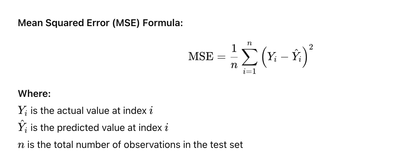
Interpretation: MSE gives more weight to larger errors because the errors are squared. This means that models with even a few very large errors will have a significantly higher MSE. A lower MSE indicates a better fit. The unit of MSE is the square of the unit of the data (e.g., if you’re forecasting temperature in Celsius, MSE is in Celsius squared).
Let’s walk through a simple numerical example for MSE calculation.
Numerical Example:
Suppose we have the following actual values and predictions for a small test set:
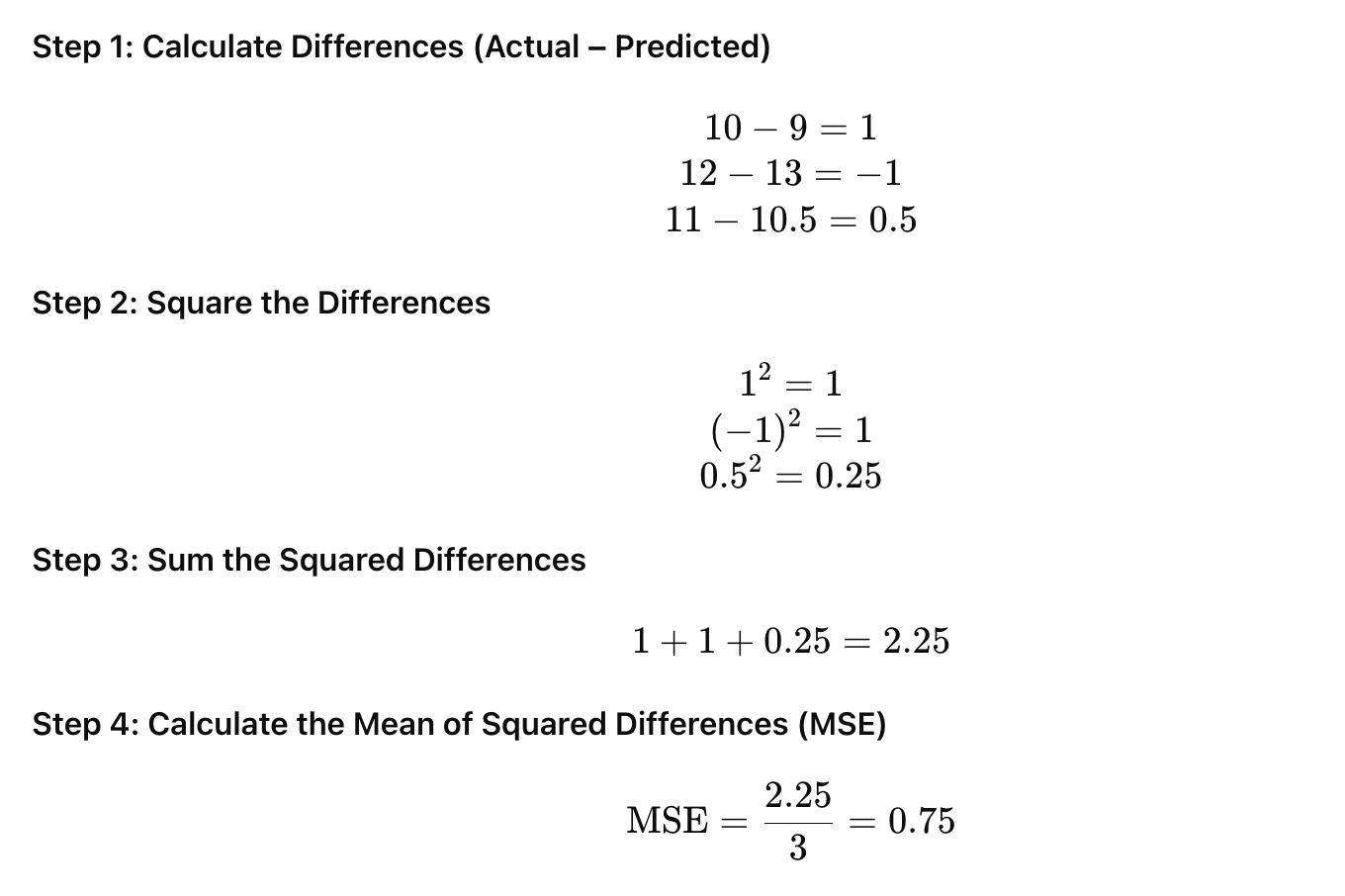
Now, let’s implement this in Python. We’ll simulate some predictions for our test_data.
# 3. Simulate some predictions for the test data
# In a real scenario, you would train a model on 'train_data' and predict on 'test_data'.
# For demonstration, let's create simple dummy predictions based on the test_data itself,
# adding some noise to simulate prediction errors.
# We'll just shift the test data and add some random errors for simplicity.
# This is NOT how you'd make real predictions, but for MSE calculation it works.
dummy_predictions = test_data['Value'].shift(1).fillna(method='bfill') + np.random.normal(0, 1.5, len(test_data))# Ensure predictions are aligned with actuals (same index)
actual_values = test_data['Value']
print("\nActual Values (Test Set Head):")
print(actual_values.head())
print("\nDummy Predictions (Test Set Head):")
print(dummy_predictions.head())
Before calculating MSE, we need actual values and corresponding predictions. Since we don’t have a trained model yet, this chunk simulates dummy_predictions for the test_data. In a real scenario, dummy_predictions would be generated by your trained forecasting model. We align the actual values from test_data with these predictions.
# 4. Calculate MSE manually
squared_errors = (actual_values - dummy_predictions) ** 2
mse_manual = squared_errors.mean()
print(f"\nManual MSE Calculation: {mse_manual:.4f}")
# 5. Calculate MSE using scikit-learn's function (recommended for robustness)
mse_sklearn = mean_squared_error(actual_values, dummy_predictions)
print(f"Scikit-learn MSE Calculation: {mse_sklearn:.4f}")
# Verify they are close
assert np.isclose(mse_manual, mse_sklearn)
This final code block demonstrates two ways to calculate MSE: manually by applying the formula steps in Python, and using scikit-learn's mean_squared_error function. The scikit-learn function is generally preferred in practice due to its robustness and efficiency. We compare the results to ensure consistency.
Other Common Error Metrics:
While MSE is widely used, it’s often beneficial to consider other metrics, as each provides a slightly different perspective on model performance.
Root Mean Squared Error (RMSE):

Interpretation: RMSE is simply the square root of MSE. Its main advantage is that it’s in the same units as the original time series, making it more interpretable than MSE. Like MSE, it penalizes large errors more heavily.
Mean Absolute Error (MAE):
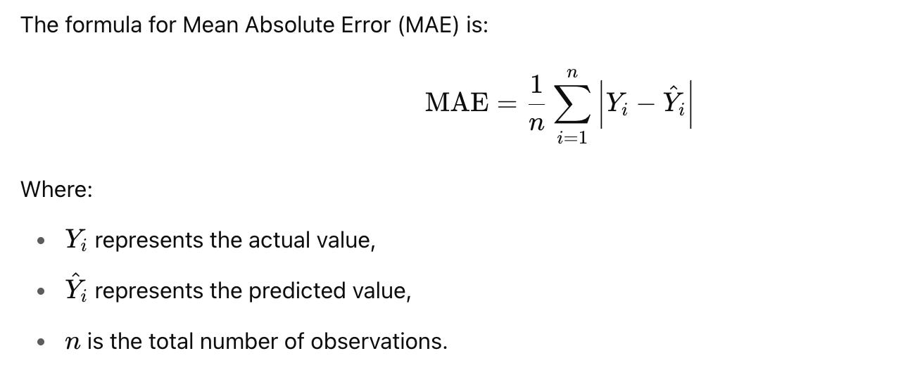
Interpretation: MAE calculates the average of the absolute differences between predictions and actuals. It is less sensitive to outliers than MSE or RMSE because it doesn’t square the errors. It provides a straightforward average magnitude of error, in the same units as the data.
Pros: Easy to understand, robust to outliers.
Cons: Does not penalize large errors as much as MSE/RMSE, which might be undesirable if large errors are particularly costly.
Mean Absolute Percentage Error (MAPE):
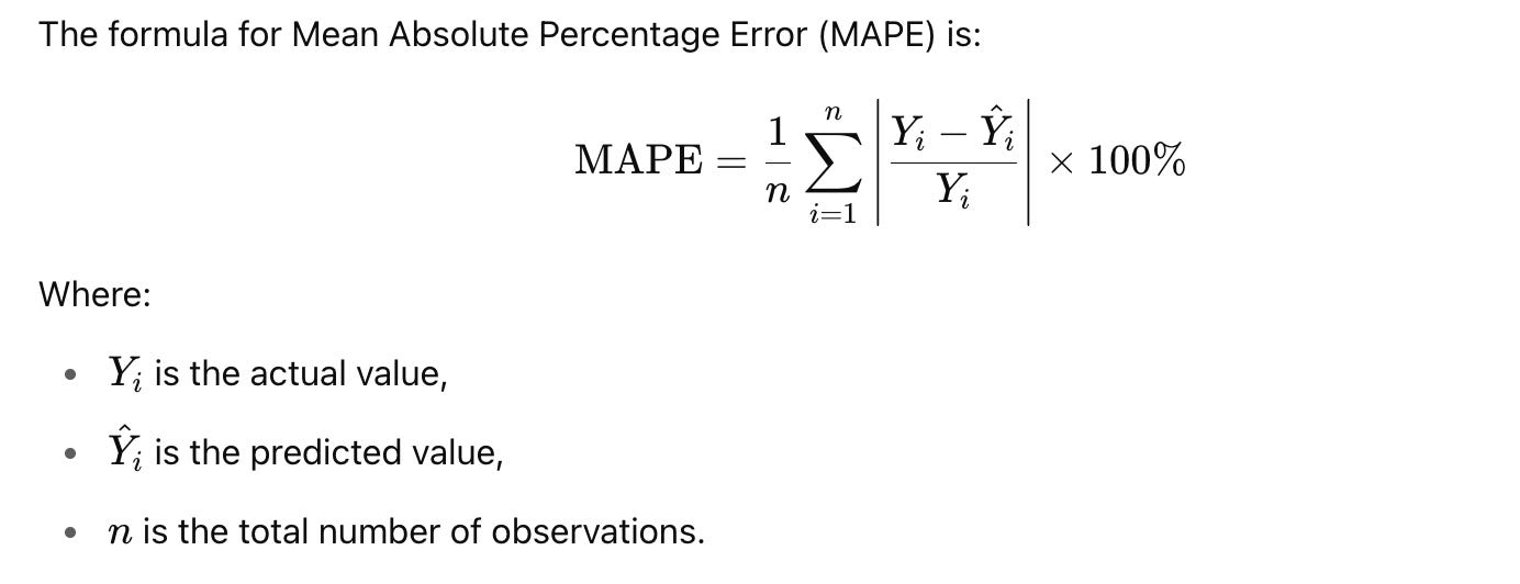
Interpretation: MAPE expresses the error as a percentage of the actual value. This makes it useful for comparing forecast accuracy across different time series or datasets that have different scales.
Pros: Scale-independent, intuitive percentage interpretation.
Cons: Undefined or infinite when actual values ($Y_i$) are zero. Can be unstable when actual values are very close to zero, leading to extremely large percentage errors even for small absolute errors. It also implicitly assumes that an error of a certain percentage is equally important across all scales.
When to prefer which metric:
MSE/RMSE: When large errors are particularly undesirable and you want your model to be heavily penalized for them (e.g., financial forecasting where large errors can lead to significant losses).
MAE: When you want a robust measure of average error magnitude, less influenced by outliers, and interpretability in the original units is key.
MAPE: When you need a scale-independent metric to compare performance across different datasets or when errors are best understood as percentages of the actual values (e.g., sales forecasting). Be cautious with values near zero.
Comparative Analysis and Model Selection
After evaluating multiple candidate models using one or more error metrics, you’ll need to compare their performance. The model with the lowest error on the test set is generally considered the “best” model for your specific problem and data. However, selection isn’t always solely based on the lowest error metric. Other factors include:
Interpretability: Can you understand why the model makes certain predictions? Statistical models often offer higher interpretability.
Computational Cost: How long does it take to train and make predictions? Deep learning models can be very resource-intensive.
Robustness: How well does the model perform under slight variations or noise in the data?
Ease of Maintenance/Deployment: How simple is it to update the model with new data or integrate it into existing systems?
It’s often a trade-off. A slightly less accurate but much more interpretable or computationally efficient model might be preferred over a marginally more accurate but opaque and complex one, especially in business contexts where understanding and trust are critical.
Beyond Single Train-Test Splits: Walk-Forward Validation
While a single train-test split is a good starting point, it only provides one snapshot of performance. For more robust evaluation, especially with limited data or when dealing with evolving time series, walk-forward validation (also known as rolling forecast origin) is a superior strategy.
In walk-forward validation:
You train your model on an initial segment of the time series.
You forecast for the next immediate period (e.g., the next day or week).
You then “walk forward” by adding the actual observed value for that period to your training data.
You retrain the model (or update it) and forecast the next period.
This process repeats, simulating a real-time forecasting scenario and providing a more reliable estimate of model performance over various historical periods. While more computationally intensive, it offers a much richer understanding of your model’s stability and generalization ability.
Deploying to Production
Once a “champion” forecasting model has been developed and thoroughly validated, the next crucial step is to deploy it to a production environment. This transition marks the shift from an experimental, development-focused phase to making the model operational and accessible for practical use. Deploying a model means making it available for automated predictions without requiring manual intervention, allowing it to seamlessly integrate into existing business processes or applications.
The ultimate goal of deployment is to enable the model to consistently take in new data and return predictions, serving a specific business need or end-user application. This automation ensures that forecasts are generated reliably, consistently, and at scale, transforming insights from the model into actionable intelligence.
Deployment Paradigms: Batch vs. Real-time Inference
The choice of deployment strategy heavily depends on how and when predictions are needed. We typically differentiate between two primary paradigms: batch inference and real-time (or online) inference.
Batch Inference
Batch inference involves making predictions on a large collection of data points at once, typically on a scheduled basis. The model processes the entire batch, and the generated forecasts are then stored or delivered for later use.
Characteristics:
Latency: High latency is acceptable, as predictions are not needed instantaneously.
Throughput: Focus is on processing large volumes of data efficiently.
Use Cases: Nightly sales forecasts, monthly budget projections, weekly inventory reordering, or any scenario where predictions can be pre-calculated.
Example Use Case: A retail company generating sales forecasts for the next quarter on a weekly basis. The model runs on a server, processes historical sales data along with any new relevant information (e.g., marketing campaigns), and then updates a database with the projected sales figures. Business analysts or dashboards then pull these pre-calculated forecasts.
Real-time (Online) Inference
Real-time inference involves making predictions on individual data points as they arrive, providing forecasts almost instantaneously. This requires the model to be constantly running and ready to receive new inputs.
Characteristics:
Latency: Low latency is critical, as predictions are needed immediately.
Throughput: Focus is on handling individual requests rapidly.
Use Cases: Predicting demand for a ride-sharing service as a new request comes in, recommending products to a user browsing an e-commerce site, or real-time fraud detection.
Example Use Case: A weather application that displays temperature forecasts for a specific location. When a user requests the forecast, the application sends the location data to a deployed model, which then returns the prediction instantly to be displayed to the user.
Common Model Deployment Approaches
The method of deployment chosen depends on the specific requirements of the application, the existing infrastructure, and the scale of operations.
Model as an API (Application Programming Interface)
One of the most common and flexible ways to deploy a forecasting model is by exposing it as a RESTful API. This allows other applications (web applications, mobile apps, internal systems, dashboards) to send data to the model and receive predictions back programmatically.
Advantages:
Interoperability: Language and platform agnostic, allowing diverse systems to consume predictions.
Scalability: Can be scaled independently of the consuming applications.
Modularity: Encapsulates the model’s logic, making it easier to update or replace.
Conceptual Flow:
A client application sends a request (e.g., HTTP POST) with input data to a specific API endpoint. A server hosts the model, processes the input using the model, and returns the prediction in a structured format (e.g., JSON).
Let’s illustrate with a minimal Python example using Flask (a micro-web framework) to serve a dummy forecasting model. In a real-world scenario, your trained model (e.g., a Prophet model or ARIMA model) would be loaded from a file.
First, we need a “dummy” model and some “dummy” data to simulate a forecasting scenario. We’ll use scikit-learn for a simple linear regression model as a placeholder for a time series model, as the focus here is on the deployment mechanism.
# Import necessary libraries
import joblib
import pandas as pd
from sklearn.linear_model import LinearRegression
import numpy as np
# --- Simulate a "trained" forecasting model ---
# In a real scenario, you would load your pre-trained model here.
# For demonstration, let's create a simple linear regression model.
# This model will predict a 'target' based on an 'input_feature'.
print("Simulating model training and saving...")
# Create dummy data for training
np.random.seed(42)
X_train = np.random.rand(100, 1) * 10 # 100 samples, 1 feature
y_train = 2 * X_train + 1 + np.random.randn(100, 1) * 2 # y = 2x + 1 + noise
# Train a simple linear regression model
dummy_model = LinearRegression()
dummy_model.fit(X_train, y_train)
# Save the dummy model to a file (e.g., 'model.pkl')
# This is how you would typically load your trained model in production.
model_filename = 'dummy_forecasting_model.pkl'
joblib.dump(dummy_model, model_filename)
print(f"Dummy model saved to {model_filename}")
This initial code segment simulates the crucial step of having a trained model ready for deployment. We create a simple LinearRegression model, train it on some dummy data, and then save it to a file using joblib. In a real forecasting project, dummy_forecasting_model.pkl would be your actual time series model (e.g., a Prophet model, SARIMA, or a custom deep learning model) that you spent time developing and validating. Saving it allows the deployment environment to load it without retraining.
Next, we’ll set up a Flask application to serve this model via a REST API.
# Import Flask for creating the web service
from flask import Flask, request, jsonify
import joblib # To load the pre-trained model
# --- Flask Application Setup ---
app = Flask(__name__) # Initialize the Flask application
# Load the pre-trained model when the application starts
# This ensures the model is loaded once into memory, not on every request.
try:
    model = joblib.load('dummy_forecasting_model.pkl')
    print("Dummy forecasting model loaded successfully.")
except Exception as e:
    print(f"Error loading model: {e}")
    model = None # Handle case where model loading fails
This part of the code initializes our Flask application and, critically, loads the pre-trained model into memory. Loading the model once when the application starts is a best practice for efficiency, as it avoids the overhead of loading it for every incoming prediction request. Error handling for model loading is also included to make the setup more robust.
Now, we define the API endpoint that will receive data and return predictions.
# --- API Endpoint for Predictions ---
@app.route('/predict', methods=['POST'])
def predict():
    if model is None:
        return jsonify({"error": "Model not loaded. Please check server setup."}), 500
# Get data from the request
    # Expecting JSON data like: {"input_feature": 5.0}
    data = request.get_json(force=True)
    # Validate input data
    if 'input_feature' not in data:
        return jsonify({"error": "Missing 'input_feature' in request."}), 400
    try:
        # Convert input to a format the model expects (e.g., a 2D array for scikit-learn)
        input_value = np.array(data['input_feature']).reshape(1, -1)
        # Make prediction using the loaded model
        prediction = model.predict(input_value)[0][0] # Adjust indexing based on model output
        # Return the prediction as JSON
        return jsonify({"forecast": prediction})
    except Exception as e:
        # Log the error for debugging
        print(f"Prediction error: {e}")
        return jsonify({"error": "An error occurred during prediction."}), 500
This is the core of our API. The @app.route('/predict', methods=['POST']) decorator registers the predict function to handle POST requests to the /predict URL path. Inside the function, it retrieves JSON data from the incoming request, validates it, prepares the data in the format expected by the scikit-learn model (a 2D array), makes the prediction, and then returns the forecast as a JSON response. Robust error handling is included to manage cases of missing models, malformed input, or prediction failures.
Finally, we add the code to run the Flask application.
# --- Run the Flask Application ---
if __name__ == '__main__':
    # For production, consider using a more robust WSGI server like Gunicorn or uWSGI
    # app.run(debug=True) # debug=True is for development, not production
    print("Flask app starting. Access at http://127.0.0.1:5000/predict (POST requests)")
    app.run(host='0.0.0.0', port=5000) # Listen on all available interfaces
This final chunk ensures that the Flask application runs when the script is executed directly. In a production environment, you would typically use a more robust WSGI (Web Server Gateway Interface) server like Gunicorn or uWSGI to run your Flask application, which provides better performance, stability, and process management. The host='0.0.0.0' setting makes the server accessible from external machines on the network, which is necessary for deployment beyond your local machine.
To test this API, you could send a POST request using curl or a tool like Postman:
curl -X POST -H "Content-Type: application/json" -d '{"input_feature": 7.5}' http://127.0.0.1:5000/predictThis would return a JSON response similar to {"forecast": 16.0} (the exact value depends on your dummy model's training).
Batch Processing via Scheduled Jobs
For batch inference, models are often deployed as part of a scheduled job or pipeline. This involves a script that runs periodically, loads the model, fetches new data, generates forecasts, and then stores or distributes these forecasts.
Advantages:
Simplicity: Can be simpler to set up than real-time APIs for non-interactive needs.
Resource Efficiency: Resources are only consumed during the scheduled run.
Scalability: Can process very large datasets by leveraging distributed computing frameworks (e.g., Apache Spark).
Conceptual Flow:
A scheduler (e.g., Cron on Linux, Windows Task Scheduler, Airflow, Prefect) triggers a Python script. The script connects to a data source, loads the model, makes predictions, and writes the results to a database, file, or sends them as a report.
Here’s a simplified Python script that simulates a batch forecasting process:
import joblib
import pandas as pd
import numpy as np
from datetime import datetime, timedelta
# --- Configuration ---
MODEL_PATH = 'dummy_forecasting_model.pkl'
INPUT_DATA_PATH = 'new_data_for_forecast.csv'
OUTPUT_FORECAST_PATH = 'batch_forecast_results.csv'
# --- Simulate New Data Arrival ---
# In a real scenario, this would fetch new data from a database or data lake.
print("Simulating new data arrival...")
# Create dummy data for new predictions
num_new_points = 5
new_input_features = np.random.rand(num_new_points, 1) * 10
# Create a DataFrame for the new data, assuming a timestamp column
new_data_df = pd.DataFrame(new_input_features, columns=['input_feature'])
new_data_df['timestamp'] = [datetime.now() + timedelta(days=i) for i in range(num_new_points)]
new_data_df.to_csv(INPUT_DATA_PATH, index=False)
print(f"New data saved to {INPUT_DATA_PATH}")
This initial part sets up configuration variables and simulates the arrival of new data that needs forecasting. In a production environment, new_data_for_forecast.csv might be a table in a data warehouse or a stream of events. We generate a few random input features and associate them with timestamps, then save this to a CSV file to simulate new data.
Next, the script will load the model and the new data, perform predictions, and save the results.
# --- Load Model and New Data ---
print("Loading model and new data...")
try:
    model = joblib.load(MODEL_PATH)
    new_data = pd.read_csv(INPUT_DATA_PATH)
    print("Model and new data loaded successfully.")
except FileNotFoundError:
    print(f"Error: Model file '{MODEL_PATH}' or data file '{INPUT_DATA_PATH}' not found.")
    exit()
except Exception as e:
    print(f"Error loading files: {e}")
    exit()
# Prepare data for prediction
# Assuming 'input_feature' is the column used by the model
features_for_prediction = new_data[['input_feature']].values
Here, the script loads the pre-trained model and the newly arrived data. It includes basic error handling for FileNotFoundError and other exceptions. The features_for_prediction are extracted, ensuring they are in the correct format (e.g., a NumPy array) for the model's predict method.
Finally, the predictions are made and saved.
# --- Make Predictions ---
print("Making predictions...")
try:
    predictions = model.predict(features_for_prediction)
    # Flatten predictions if they are nested arrays (common with scikit-learn)
    predictions = predictions.flatten()
    print("Predictions generated.")
except Exception as e:
    print(f"Error during prediction: {e}")
    exit()
# --- Store Results ---
# Add predictions to the DataFrame and save
new_data['forecast'] = predictions
new_data.to_csv(OUTPUT_FORECAST_PATH, index=False)
print(f"Forecasts saved to {OUTPUT_FORECAST_PATH}")
print("Batch forecasting process completed.")
This section executes the predict method of the loaded model on the new data. The resulting predictions are then added as a new column to the new_data DataFrame, and the entire DataFrame, now including the forecasts, is saved to a new CSV file. In a production setting, this output might be written to a database table, a data lake, or sent to a reporting tool. This script would then be scheduled to run at regular intervals.
3. Integration into Web Applications or Dashboards
While often leveraging an API backend, a forecasting model can also be directly integrated into a user-facing web application or business intelligence dashboard. This provides a graphical interface for users to input data, visualize forecasts, or interact with the model’s output.
Conceptual Flow:
A user interacts with a dashboard. Behind the scenes, the dashboard’s backend either directly loads and runs the model (less common for large models) or, more typically, calls a dedicated model API (as described above) to retrieve forecasts. The results are then rendered visually for the user.
4. Embeddable Models (e.g., Excel Functions, Edge Devices)
In some specialized cases, models might be converted into formats that can be embedded directly into applications or devices that traditionally don’t host complex machine learning environments. This aligns with the professor’s mention of “Excel functions.”
Excel/Spreadsheets: Tools like ONNX (Open Neural Network Exchange) or PMML (Predictive Model Markup Language) allow models trained in various frameworks to be exported into a portable format that can then be imported and run within applications like Excel, often via specific add-ins or custom functions. This allows business users to interact with the model directly in their familiar environment.
Edge Devices: For IoT (Internet of Things) applications, models might be optimized and deployed directly onto small, low-power devices (e.g., smart sensors) to make real-time predictions without needing to send data back to a central server. This is common for predictive maintenance on machinery or localized weather predictions.
Key Considerations for Production Deployment
Deploying a model to production involves more than just making predictions. Several critical factors must be addressed to ensure the system is robust, reliable, and performs well under real-world conditions.
Scalability
A production system must be able to handle varying loads, from a few requests per hour to thousands per second.
Horizontal Scaling: Adding more instances of the model service behind a load balancer to distribute incoming requests.
Auto-scaling: Automatically adjusting the number of instances based on traffic load, common in cloud environments.
Resource Allocation: Ensuring sufficient CPU, memory, and GPU resources are available for the model to run efficiently.
Latency
For real-time applications, the time it takes for a model to receive input, process it, and return a prediction (latency) is crucial.
Optimization: Using optimized model formats, efficient code, and fast inference engines.
Proximity: Deploying model services geographically closer to the users or data sources.
Caching: Caching frequently requested forecasts or pre-computing predictions where possible.
Reliability and High Availability
Production systems must be resilient to failures and available around the clock.
Redundancy: Deploying multiple instances of the model service across different servers or data centers.
Load Balancers: Distributing traffic and rerouting requests away from unhealthy instances.
Failover Mechanisms: Automated systems to switch to backup services in case of primary system failure.
Fault Tolerance: Designing the system to continue operating even if individual components fail.
Security
Exposing a model via an API introduces security risks that must be mitigated.
Authentication & Authorization: Ensuring only authorized users or systems can access the model. This might involve API keys, OAuth tokens, or other identity management systems.
Input Validation: Sanitize and validate all incoming data to prevent injection attacks or unexpected model behavior due to malformed inputs.
Data Encryption: Encrypting data in transit (HTTPS) and at rest to protect sensitive information.
Network Security: Using firewalls, virtual private clouds (VPCs), and other network controls to restrict access.
Version Control and Rollbacks
As models are continuously improved, managing different versions is essential.
Model Registry: A centralized repository for storing, versioning, and managing trained models.
Deployment Pipelines: Automated processes that allow for seamless deployment of new model versions and quick rollbacks to previous versions if issues arise.
A/B Testing/Canary Deployments: Gradually rolling out new model versions to a small subset of users to evaluate performance before full deployment.
Monitoring (Brief Introduction)
While the next section will delve deeper into monitoring, it’s critical to understand its importance immediately after deployment.
Performance Monitoring: Tracking the technical health of the deployed service (e.g., latency, error rates, resource utilization).
Model Performance Monitoring: Crucially, tracking the accuracy and relevance of the model’s predictions over time. This involves comparing forecasts against actual outcomes once they become available.
Data Drift: Monitoring changes in the characteristics of the input data compared to the data the model was trained on. Significant drift can degrade model performance.
Concept Drift: Monitoring changes in the relationship between input features and the target variable itself. This indicates that the underlying patterns the model learned are no longer valid.
Introduction to MLOps (Machine Learning Operations)
The complexities of deploying, managing, and monitoring machine learning models in production have given rise to the discipline of MLOps. MLOps is a set of practices that combines Machine Learning, DevOps, and Data Engineering to standardize and streamline the entire machine learning lifecycle, from experimentation and development to deployment and maintenance.
Key Principles of MLOps:
Automation: Automating model training, testing, deployment, and monitoring.
Reproducibility: Ensuring that models and their results can be consistently reproduced.
Version Control: Managing code, data, and models in a versioned manner.
Continuous Integration/Continuous Delivery (CI/CD): Applying software engineering CI/CD principles to machine learning pipelines, allowing for frequent and reliable model updates.
Monitoring and Alerting: Proactive tracking of model and infrastructure performance.
Common tools and platforms supporting MLOps include Docker (for containerization), Kubernetes (for container orchestration), Apache Airflow (for workflow management), and cloud-specific ML platforms like AWS SageMaker, Azure Machine Learning, and Google Cloud AI Platform. These tools provide the infrastructure and services needed to build robust and scalable model deployment pipelines.
Conceptual Deployment Architecture
A typical conceptual architecture for deploying a forecasting model might look like this:
+----------------+       +-------------------+       +--------------------+       +-----------------+
| Data Sources   | ----> | Data Ingestion/   | ----> | Prediction Service | ----> | Application/    |
| (Databases,     |       | Preprocessing     |       | (Deployed Model)   |       | Dashboard/      |
| APIs, Files)   |       | (e.g., ETL jobs)  |       | (API, Batch Script)|       | Reporting       |
+----------------+       +-------------------+       +--------------------+       +-----------------+
        ^                               ^                        |                        ^
        |                               |                        |                        |
        |                               |                        |                        |
+----------------+       +--------------------+       +--------------------+       +-----------------+
| External Users | <---- | Web Application/   | <---- | API Gateway/       | <---- | Monitoring &    |
| (via UI)       |       | Dashboard Backend  |       | Load Balancer      |       | Alerting System |
+----------------+       +--------------------+       +--------------------+       +-----------------+
In this flow:
Data Sources provide the input data required for forecasting.
Data Ingestion/Preprocessing pipelines clean, transform, and prepare this data for the model.
The Prediction Service (your deployed model) consumes the prepared data and generates forecasts. This could be an API endpoint for real-time requests or a scheduled batch script.
The forecasts are then consumed by a Reporting, Dashboard, or Application layer, making them accessible to end-users or other systems.
For external access, an API Gateway/Load Balancer manages incoming requests, routes them to the correct prediction service instance, and handles security.
A Monitoring & Alerting System continuously tracks the health and performance of the entire pipeline, ensuring the model remains accurate and operational.
Deploying to production is a critical milestone that brings your forecasting model to life, enabling it to deliver continuous value. It transitions the model from an analytical artifact to an integral, automated component of a larger system, laying the groundwork for ongoing monitoring and continuous improvement.
Monitoring
Once a time series forecasting model has been developed, rigorously tested, and deployed into a production environment, the journey is far from over. In fact, a critical and continuous phase begins: monitoring. Monitoring a deployed forecasting model is essential to ensure its continued accuracy, reliability, and value in real-world scenarios. Without robust monitoring, even the most sophisticated model can silently degrade in performance, leading to poor decision-making and potentially significant business losses.
The Necessity of Continuous Monitoring
The core purpose of monitoring is to assess how well the model’s forecasts align with the actual observed values over time. Unlike a static analytical report, a deployed model operates in a dynamic environment where underlying patterns can shift, external factors can intervene, and data quality issues can emerge. Monitoring acts as an early warning system, allowing practitioners to detect deviations, diagnose root causes, and take corrective actions before problems escalate.
Consider a model forecasting daily temperature for an outdoor event planner. Initially, it might perform exceptionally well. However, an unexpected heatwave, a sudden cold snap, or even a change in sensor calibration could cause the model’s predictions to become wildly inaccurate. Without monitoring, the planner might only realize the issue after critical decisions (like staffing or inventory) have been made based on flawed forecasts.
Quantifying Forecast Quality: Key Metrics
To systematically compare forecasts to actuals and quantify performance degradation, we rely on a set of statistical metrics. These metrics provide objective measures of error and bias, allowing for consistent evaluation over time. While many metrics exist, some are particularly common in time series forecasting:
Mean Absolute Error (MAE): The average of the absolute differences between forecasts and actual values. MAE is easy to interpret as it’s in the same units as the data, but it treats all errors equally.
Mean Squared Error (MSE) / Root Mean Squared Error (RMSE): MSE calculates the average of the squared differences, penalizing larger errors more heavily. RMSE is the square root of MSE, bringing the error back into the same units as the data, making it more interpretable than MSE itself. RMSE is sensitive to outliers.
Mean Absolute Percentage Error (MAPE): Expresses the error as a percentage of the actual value. This is useful for comparing performance across different datasets or series with varying scales, but it can be problematic with zero or near-zero actual values.
Bias (Mean Error): The average of the differences between forecasts and actual values (without taking absolute values). A positive bias indicates the model generally over-predicts, while a negative bias indicates under-prediction. Bias helps identify systematic errors.
Let’s illustrate how to calculate these common metrics using Python. For this, we’ll simulate some actual and forecasted values.
import pandas as pd
import numpy as np
from sklearn.metrics import mean_absolute_error, mean_squared_error
# For reproducibility
np.random.seed(42)
# Simulate actual and forecasted values for a time series
dates = pd.date_range(start='2023-01-01', periods=100, freq='D')
actuals = np.random.rand(100) * 100 + np.sin(np.arange(100) / 10) * 20 # Some base value + seasonality
forecasts = actuals * 0.95 + np.random.randn(100) * 5 # Forecasts are close to actuals but with noise
# Create a DataFrame for easier handling
df = pd.DataFrame({'date': dates, 'actual': actuals, 'forecast': forecasts})
df.set_index('date', inplace=True)
print("Sample Data:")
print(df.head())
This initial code block sets up a simple dataset for demonstration. We generate 100 daily data points, simulating actual time series values with a trend and seasonality, and forecast values that are generally close to the actuals but include some random noise to represent prediction error. This DataFrame will serve as our basis for calculating various error metrics.
Calculating Key Error Metrics
Now, let’s calculate MAE, RMSE, MAPE, and Bias using our simulated data.
# Calculate Mean Absolute Error (MAE)
mae = mean_absolute_error(df['actual'], df['forecast'])
print(f"\nMean Absolute Error (MAE): {mae:.2f}")
# Calculate Root Mean Squared Error (RMSE)
rmse = np.sqrt(mean_squared_error(df['actual'], df['forecast']))
print(f"Root Mean Squared Error (RMSE): {rmse:.2f}")
Here, we compute MAE and RMSE. mean_absolute_error and mean_squared_error from sklearn.metrics are convenient for this. MAE gives us the average magnitude of errors, while RMSE, by squaring errors, penalizes larger errors more, making it sensitive to outliers. Both are in the same units as our original data, making them directly interpretable.
# Calculate Mean Absolute Percentage Error (MAPE)
# Custom function for MAPE as sklearn does not have a direct implementation that handles zeros well
def mean_absolute_percentage_error(y_true, y_pred):
    # Avoid division by zero by adding a small epsilon or handling cases where y_true is 0
    # For simplicity here, we'll filter out cases where y_true is 0.
    non_zero_actuals_mask = y_true != 0
    y_true_filtered = y_true[non_zero_actuals_mask]
    y_pred_filtered = y_pred[non_zero_actuals_mask]
if len(y_true_filtered) == 0:
        return np.nan # No valid actuals to calculate MAPE
    return np.mean(np.abs((y_true_filtered - y_pred_filtered) / y_true_filtered)) * 100
mape = mean_absolute_percentage_error(df['actual'], df['forecast'])
print(f"Mean Absolute Percentage Error (MAPE): {mape:.2f}%")
MAPE is particularly useful for communicating forecast accuracy in a percentage format, which is often more intuitive for business stakeholders. However, it’s crucial to handle cases where actual values are zero or very close to zero, as this can lead to division by zero or extremely large, misleading percentage errors. Our custom function includes a basic filter for non-zero actuals.
# Calculate Bias (Mean Error)
bias = np.mean(df['forecast'] - df['actual'])
print(f"Bias (Mean Error): {bias:.2f}")
Bias provides insight into whether the model systematically over-predicts or under-predicts. A positive bias indicates over-prediction on average, while a negative bias indicates under-prediction. This metric is crucial for understanding the directional tendency of the forecast errors, which might require different corrective actions than simply reducing overall error magnitude.
Visualizing Performance Over Time
While numerical metrics provide a summary, visualizing actuals versus forecasts and the errors themselves is indispensable for understanding model behavior and diagnosing issues. Visualizations can quickly reveal trends in errors, periods of poor performance, and the impact of specific events.
import matplotlib.pyplot as plt
import seaborn as sns
# Set a style for better aesthetics
sns.set_style("whitegrid")
# Plot Actuals vs. Forecasts
plt.figure(figsize=(12, 6))
plt.plot(df.index, df['actual'], label='Actuals', color='blue', alpha=0.7)
plt.plot(df.index, df['forecast'], label='Forecasts', color='red', linestyle='--', alpha=0.7)
plt.title('Actuals vs. Forecasts Over Time')
plt.xlabel('Date')
plt.ylabel('Value')
plt.legend()
plt.grid(True)
plt.tight_layout()
plt.show()
This plot is the most fundamental visualization for monitoring. By visually comparing the Actuals line to the Forecasts line, we can immediately spot periods where the model deviates significantly or consistently. For instance, if the red dashed line consistently runs above the blue line, it suggests an over-forecasting bias. If the lines suddenly diverge sharply at a specific point, it might indicate an external shock or data issue.
# Plot Forecast Errors (Residuals)
df['error'] = df['forecast'] - df['actual']
plt.figure(figsize=(12, 6))
plt.plot(df.index, df['error'], label='Forecast Error', color='purple', alpha=0.7)
plt.axhline(0, color='black', linestyle=':', linewidth=0.8) # Zero error line
plt.title('Forecast Errors Over Time')
plt.xlabel('Date')
plt.ylabel('Error (Forecast - Actual)')
plt.legend()
plt.grid(True)
plt.tight_layout()
plt.show()
Plotting the Forecast Error (residuals) directly helps in identifying patterns in the errors themselves. Ideally, errors should be randomly distributed around zero. Trends (e.g., errors consistently increasing or decreasing), seasonality in errors, or sudden spikes indicate underlying problems with the model or the data. For example, a sustained positive error indicates consistent over-prediction.
Understanding and Diagnosing Forecast Degradation
When monitoring reveals a decline in model performance, the next crucial step is to diagnose the root cause. Degradation can stem from several factors, often categorized into:
Data Drift
Data drift refers to changes in the distribution of the input data (features) that the model receives. The world evolves, and the characteristics of the data used for forecasting can shift. For example, if a sales forecasting model was trained on data where most transactions occurred on weekdays, but a new policy shifts a significant portion of sales to weekends, the input distribution has drifted. The model might not be well-equipped to handle these new patterns.
Concept Drift
Concept drift occurs when the underlying relationship between the input features and the target variable changes over time. The “concept” the model learned during training is no longer valid. For instance, a model predicting housing prices might learn that square footage is the primary driver. However, if a new urban development suddenly makes proximity to public transport a much stronger factor, the concept has drifted. The old relationship (square footage -> price) is less accurate, even if the square footage distribution hasn’t changed.
External Shocks and Anomalies
These are sudden, often unpredictable events that significantly impact the time series, making historical patterns irrelevant or misleading for a period. Examples include:
Economic downturns or booms: A recession can drastically alter consumer spending habits.
Policy changes: New regulations (e.g., tariffs, environmental laws) can affect supply chains or demand.
Natural disasters: Hurricanes, floods, or pandemics can disrupt normal operations and demand patterns.
Technical failures: Sensor malfunctions, data pipeline breaks, or system outages can introduce erroneous or missing data.
Major competitor actions: A new product launch or pricing strategy from a competitor can shift market dynamics.
Social events: Major holidays, sporting events, or cultural shifts can temporarily or permanently alter behavior.
It’s important to distinguish between temporary performance dips due to anomalies and sustained degradation requiring intervention. A single outlier might be an anomaly, while a consistent increase in error over weeks suggests drift.
Model Staleness
Sometimes, a model simply becomes “stale” because the world generally evolves, and the patterns it learned from historical data slowly become less representative of current reality. This is a more gradual form of concept drift, not tied to a single identifiable event but rather a continuous shift. Regular retraining or adaptive models can address staleness.
Automated Monitoring and Alerting
Manual inspection of charts and metrics is unsustainable for continuous monitoring, especially with many models. Automated monitoring systems are crucial. These systems can:
Calculate metrics periodically: Daily, hourly, or even more frequently.
Compare current performance to historical benchmarks: Is the current RMSE significantly worse than the average RMSE over the last month?
Trigger alerts: Send notifications (email, Slack, PagerDuty) if a metric crosses a predefined threshold or if data drift is detected.
Generate dashboards: Provide a consolidated view of model health and performance.
Let’s look at a simplified example of setting up a basic automated check and alert.
# Simulate a period of degraded performance
df_monitoring = df.copy()
# Introduce a period where forecasts are significantly off
df_monitoring.loc['2023-03-01':'2023-03-10', 'forecast'] = df_monitoring.loc['2023-03-01':'2023-03-10', 'actual'] * 1.5
# Define a threshold for performance degradation (e.g., if RMSE exceeds a certain value)
# This threshold would typically be determined empirically or based on business tolerance
PERFORMANCE_THRESHOLD_RMSE = 10.0
# Function to check model performance and trigger an alert
def check_model_performance(data, threshold_rmse):
    current_rmse = np.sqrt(mean_squared_error(data['actual'], data['forecast']))
    print(f"\nCurrent RMSE: {current_rmse:.2f}")
    if current_rmse > threshold_rmse:
        print(f"ALERT! Model performance degraded. RMSE ({current_rmse:.2f}) exceeds threshold ({threshold_rmse:.2f}).")
        # In a real system, you would send an email, Slack message, or log an incident.
        return True
    else:
        print("Model performance is within acceptable limits.")
        return False
# Run the check
is_degraded = check_model_performance(df_monitoring, PERFORMANCE_THRESHOLD_RMSE)
This code snippet demonstrates a basic automated check. We simulate a period of degraded performance within our dataset. The check_model_performance function calculates the current RMSE and compares it against a predefined PERFORMANCE_THRESHOLD_RMSE. If the RMSE exceeds this threshold, an alert message is printed (in a real system, this would trigger an actual notification). This simple mechanism can be scheduled to run periodically, providing continuous oversight.
Actionable Steps When Monitoring Reveals Issues
Detecting a problem is only the first step. The true value of monitoring lies in enabling timely and effective responses:
Investigate and Diagnose: Use visualizations and deeper analysis (e.g., examining specific features, looking for external event correlations) to pinpoint the exact cause of degradation (data drift, concept drift, external shock).
Retrain the Model: If the underlying data patterns have shifted significantly (data or concept drift), retraining the model on more recent, representative data is often the most effective solution. This might involve including the new, changed data in the training set.
Model Updates and Feature Engineering: If the existing model architecture is no longer suitable, or if new influential features have emerged, the model might need a more substantial update. This could involve trying different algorithms, adjusting hyperparameters, or incorporating new data sources.
Data Quality Checks: Sometimes, performance degradation is simply due to issues in the data pipeline — missing values, incorrect units, or corrupted data. Monitoring input data quality is as important as monitoring model output.
Re-evaluate Assumptions: The initial assumptions made during model development (e.g., about seasonality, trends, or external influences) might no longer hold true. A re-evaluation can lead to fundamental changes in the forecasting approach.
Temporary Intervention: For temporary external shocks, a short-term manual override or a simpler, more robust model might be deployed until the system returns to normal.
Tools and Technologies for Operational Monitoring
While our code examples use basic Python libraries, in a production environment, specialized tools and platforms are often employed for robust ML model monitoring:
MLOps Platforms: Tools like MLflow, AWS SageMaker, Azure ML, Google Cloud AI Platform, and Kubeflow offer integrated capabilities for model deployment, monitoring, and retraining pipelines.
Observability Tools: Solutions like Grafana, Prometheus, Datadog, and custom dashboards built with tools like Tableau or Power BI can visualize metrics, logs, and alerts from your forecasting systems.
Data Drift Detection Libraries: Libraries like Evidently AI, NannyML, and Fiddler AI are specifically designed to detect data and concept drift, often integrating with MLOps platforms.
Alerting Systems: PagerDuty, Opsgenie, or even simple integrations with Slack/email for critical alerts.
Monitoring is not a one-time task but an ongoing commitment. It closes the loop in the time series forecasting lifecycle, ensuring that models continue to provide accurate and valuable insights long after their initial deployment.
Collecting New Data: The Engine of Continuous Forecasting
In the dynamic landscape of real-world applications, a forecasting model is rarely a static entity. Once deployed to production and under constant monitoring, it eventually requires new data to maintain its accuracy and relevance. This continuous collection of new data forms a crucial feedback loop in the forecasting project roadmap, ensuring that models remain adaptive and performant in the face of changing conditions.
The Iterative Forecasting Lifecycle
The forecasting process is not a linear path but an iterative cycle. After a model is developed, deployed, and monitored, the insights gained from monitoring (e.g., declining performance, detected data shifts) feed directly back into the data collection phase. This initiates a new cycle of model retraining and redeployment, creating a robust, self-improving system. This continuous feedback loop is fundamental to maintaining high-quality forecasts over time.
Why Continuous Data Collection is Essential
The necessity of continuously collecting new data stems from several critical factors that impact a model’s long-term viability:
Addressing Model Staleness: Forecasts are based on historical patterns. As time progresses, the “history” on which a model was trained becomes less representative of the current reality. Without fresh data, a model becomes stale, leading to increasingly inaccurate predictions. Imagine a retail demand forecasting model trained on pre-pandemic sales data trying to predict post-pandemic demand; its accuracy would severely degrade without new data reflecting the shift in consumer behavior.
Adapting to Evolving Patterns: Economic conditions, consumer preferences, technological advancements, and even seasonal patterns can subtly or dramatically shift over time. New data captures these evolving trends, allowing the model to learn and adapt its internal representations. For instance, a model predicting energy consumption must adapt to the increasing adoption of renewable energy sources or changes in appliance efficiency standards.
The Concept of Data Drift and Model Drift: These are perhaps the most compelling reasons for continuous data collection and retraining.
Data Drift: Occurs when the statistical properties of the input data (features) or the relationship between inputs and outputs (target variable) change over time.
Covariate Shift: The distribution of the input features changes. For example, if a model predicts stock prices based on trading volume, and suddenly the average daily trading volume significantly increases across the market, the model might struggle because the input distribution has shifted.
Concept Drift: The relationship between the input features and the target variable changes. For example, in a fraud detection model, the patterns of fraudulent transactions might evolve as fraudsters find new ways to exploit systems, meaning the “concept” of fraud itself has changed.
Model Drift: A direct consequence of data drift. As the underlying data distribution changes, the model’s learned patterns (its “concepts”) no longer accurately reflect the current reality, leading to a decline in its predictive performance. Continuous data collection and retraining are the primary mechanisms to counteract both data and model drift.
Methods and Tools for Automated Data Collection
In a production environment, manual data collection is impractical and prone to errors. Automation is key. Here are common methods and tools:
Database Integrations: Many applications store their operational data in relational databases (e.g., PostgreSQL, MySQL, SQL Server) or NoSQL databases (e.g., MongoDB, Cassandra). Automated scripts or ETL (Extract, Transform, Load) pipelines can regularly query these databases to pull new transactional data, sensor readings, or user interactions.
APIs (Application Programming Interfaces): For external data sources (weather data, stock prices, social media trends, competitor pricing), APIs provide a programmatic way to fetch data. Scheduled jobs can call these APIs to retrieve the latest information.
Streaming Data Platforms: For high-velocity, real-time data, platforms like Apache Kafka, Amazon Kinesis, or Google Cloud Pub/Sub are used. These systems allow data to be continuously ingested and processed as it arrives, making it available for near-real-time forecasting or immediate appending to historical datasets.
Web Scraping: While less robust and more prone to breakage, web scraping can be used to collect data from websites that do not offer an API. This typically involves using libraries like
BeautifulSouporScrapyto parse HTML content.Flat Files and Cloud Storage: Data might arrive in structured flat files (CSV, Parquet) uploaded to cloud storage buckets (e.g., AWS S3, Google Cloud Storage, Azure Blob Storage). Automated processes can monitor these locations and ingest new files.
Triggers for New Data Collection and Retraining
Deciding when to collect new data and retrain a model is crucial. Common triggers include:
Scheduled Intervals: The simplest approach. Models might be retrained daily, weekly, monthly, or quarterly, depending on the data’s volatility and the business’s needs. This provides a predictable cadence for updates.
Performance Degradation Thresholds: Monitoring systems can track key performance metrics (e.g., RMSE, MAE, R-squared). If a metric falls below a predefined threshold, it can trigger an alert and initiate a retraining process.
Detection of Data Drift: Advanced monitoring tools can analyze incoming data streams for shifts in statistical properties (e.g., mean, variance, distribution shape) or changes in feature importance. When significant drift is detected, it signals the need for retraining.
External Events/Business Triggers: Specific business events can necessitate retraining. For example, a major marketing campaign, the launch of a new product line, a significant policy change, or an unforeseen global event (like a pandemic) might require immediate model updates.
Practical Demonstration: Simulating New Data Arrival and Appending
To illustrate the concept of new data collection and appending, let’s simulate a time series dataset representing daily sales. We’ll start with an initial dataset and then simulate new data arriving daily, appending it to our existing records.
First, we’ll create a synthetic initial dataset using pandas.
import pandas as pd
import numpy as np
# Set a random seed for reproducibility
np.random.seed(42)
# --- Initial Dataset Setup ---
# Define the start and end dates for the initial dataset
start_date_initial = '2023-01-01'
end_date_initial = '2023-01-31'
# Create a date range for January 2023
dates_initial = pd.date_range(start=start_date_initial, end=end_date_initial, freq='D')
# Simulate daily sales data with a base trend and some noise
# Let's assume a slight upward trend over the month
base_sales = np.linspace(100, 150, len(dates_initial))
noise = np.random.normal(loc=0, scale=10, size=len(dates_initial))
initial_sales = (base_sales + noise).astype(int)
# Create the initial DataFrame
initial_df = pd.DataFrame({'Date': dates_initial, 'Sales': initial_sales})
initial_df.set_index('Date', inplace=True)
print("--- Initial Sales Data (January 2023) ---")
print(initial_df.head())
print(f"Initial dataset size: {len(initial_df)} records")
This initial code block sets up our baseline dataset, simulating daily sales for January 2023. We create a DataFrame with a Date index and a Sales column, representing the historical data our model would have been trained on.
Now, let’s simulate new data arriving for a few days in February and append it to our existing dataset.
# --- Simulate New Data Arrival ---
# Define the start and end dates for new data
# Let's simulate data for the first 5 days of February
start_date_new = '2023-02-01'
end_date_new = '2023-02-05'
# Create a date range for the new data
dates_new = pd.date_range(start=start_date_new, end=end_date_new, freq='D')
# Simulate new daily sales data, perhaps with a slightly different trend or level
# Continuing the upward trend but maybe with more variability
base_sales_new = np.linspace(155, 170, len(dates_new)) # Slightly higher base
noise_new = np.random.normal(loc=0, scale=15, size=len(dates_new)) # More noise
new_sales = (base_sales_new + noise_new).astype(int)
# Create the DataFrame for new data
new_df = pd.DataFrame({'Date': dates_new, 'Sales': new_sales})
new_df.set_index('Date', inplace=True)
print("\n--- New Sales Data (First 5 Days of February 2023) ---")
print(new_df)
This second chunk generates a small batch of “new” sales data, simulating what might arrive from a daily data feed. Notice that we’ve intentionally varied the base sales and noise slightly to mimic real-world fluctuations.
Finally, we append this new data to our initial_df, demonstrating the continuous data collection process.
# --- Appending New Data to the Existing Dataset ---
# Use pandas.concat to append the new data to the initial dataset
# axis=0 means appending rows
# ignore_index=False is default, keeping the date index
combined_df = pd.concat([initial_df, new_df])
print("\n--- Combined Sales Data After Appending ---")
print(combined_df.tail(10)) # Show the last 10 entries to see the new data
print(f"Combined dataset size: {len(combined_df)} records")
# Verify that the index is unique and sorted (important for time series)
print(f"Is index unique? {combined_df.index.is_unique}")
print(f"Is index sorted? {combined_df.index.is_monotonic_increasing}")
The pd.concat function is a common and efficient way to append new time series data. After this operation, combined_df now contains both the original January data and the newly "collected" February data, ready for potential retraining. In a real system, this combined dataset might then be saved back to a data warehouse or used directly by a retraining pipeline.
Managing Model Versions
Once a model is retrained with new data, it becomes a new version of the model. Effective version management is critical in a production environment:
Reproducibility: Being able to revert to previous model versions if a new one performs poorly is essential.
Auditability: Tracking which data was used to train which model version, and when, is vital for debugging and compliance.
A/B Testing: New model versions can be tested against older ones in a live environment to confirm performance improvements before full rollout.
Tools like MLflow, DVC (Data Version Control), or dedicated MLOps platforms provide functionalities for tracking model artifacts, parameters, and performance metrics across different versions.
Computational Resources and Trade-offs
Continuous retraining is not without its costs and complexities:
Infrastructure Requirements: Retraining models, especially complex deep learning models on large datasets, requires significant computational resources (CPUs, GPUs, memory). This necessitates robust cloud infrastructure or on-premise compute clusters.
Cost: The computational resources translate directly into operational costs. Cloud providers charge for compute time, storage, and data transfer.
Complexity: Building automated data pipelines, retraining triggers, model versioning systems, and CI/CD (Continuous Integration/Continuous Deployment) pipelines adds significant engineering overhead.
Latency: The time it takes to retrain and redeploy a model can vary from minutes to hours. For very fast-changing environments, this latency might still be too high.
Trade-offs: The decision on retraining frequency involves a trade-off between model accuracy (more frequent retraining generally means higher accuracy) and cost/complexity. A business must evaluate the value of increased accuracy against the resources required. For some applications, weekly retraining might be sufficient, while others might demand daily or even hourly updates.
Addressing Cold Start Problems
A “cold start” problem occurs when there is insufficient historical data to train a robust model, often for new products, services, or locations. When collecting new data for a new series, strategies include:
Proxy Data: Using data from similar existing products or services as a proxy until enough specific data accumulates.
Rule-Based Models: Starting with simple, expert-defined rules or statistical averages until data allows for more sophisticated models.
Transfer Learning: If applicable, using a pre-trained model from a related domain and fine-tuning it with the limited new data.
Hierarchical Forecasting: If the new series is part of a larger hierarchy, forecasting at a higher aggregate level and disaggregating.
Real-World Applications
The continuous collection of new data and subsequent model retraining is critical across numerous industries:
Retail Demand Forecasting: Daily sales data, promotional impacts, and even weather patterns are continuously collected to refine predictions for inventory management, staffing, and marketing campaigns.
Energy Consumption Prediction: Real-time sensor data from smart grids, weather forecasts, and historical consumption patterns are fed into models to optimize power generation and distribution.
Financial Market Prediction: High-frequency trading models continuously ingest new tick data, news sentiment, and economic indicators to adapt to rapidly changing market conditions.
Fraud Detection: New transaction data, evolving fraud patterns, and user behavior logs are constantly collected to update models that identify suspicious activities. As fraudsters adapt, the models must too.
Healthcare Outcome Prediction: Patient vital signs, treatment responses, and epidemiological data are continuously collected to improve models for disease progression, patient risk assessment, and resource allocation.
How Time Series Forecasting is Different from Other Regression Tasks
While time series forecasting might superficially resemble standard regression problems, its fundamental nature introduces unique challenges and necessitates specialized approaches. The core distinction lies in the inherent temporal structure and dependencies within time series data, which violate assumptions commonly made in traditional regression.
Temporal Dependence: The Core Distinction
In most standard regression tasks, a critical assumption is that observations are independent and identically distributed (i.i.d.). This means that each data point is drawn independently from the same underlying distribution. For example, when predicting house prices, the price of one house is generally assumed not to directly depend on the price of a house sold a month ago in a different neighborhood, beyond shared market conditions captured by features.
Time series data, however, inherently violates this i.i.d. assumption. The value of a variable at a given time point is often highly dependent on its past values and the values of other variables at preceding time points. This characteristic is known as temporal dependence or autocorrelation.
Consider predicting tomorrow’s temperature. It’s highly probable that tomorrow’s temperature will be very close to today’s, or at least influenced by it, rather than being an entirely random draw from a distribution of all possible temperatures. This direct link to the past is what defines time series data and sets it apart.
Key Characteristics of Time Series Data
Beyond temporal dependence, several other characteristics distinguish time series forecasting:
Autocorrelation
Autocorrelation is a specific type of temporal dependence where a variable’s current value is correlated with its own past values. For instance, if you observe high electricity consumption on a weekday, it’s likely that consumption on the following weekday will also be relatively high, exhibiting a daily or weekly pattern.
Positive Autocorrelation: High values are followed by high values, and low values by low values (e.g., stock prices often trend).
Negative Autocorrelation: High values are followed by low values, and vice versa (less common in natural phenomena, but can occur in some oscillating systems).
Ignoring significant autocorrelation can lead to models that underestimate uncertainty, produce biased forecasts, or identify spurious relationships.
Stationarity
Many traditional time series models (like ARIMA) assume that the underlying statistical properties of the series, such as its mean, variance, and autocorrelation structure, remain constant over time. This property is known as stationarity.
Strict Stationarity: The joint probability distribution of any set of observations does not change over time.
Weak-Sense Stationarity (or Covariance Stationarity): The mean, variance, and autocorrelation function are constant over time.
Real-world time series data is often non-stationary. Trends (e.g., increasing population over time), seasonality (e.g., higher retail sales in December), and changing variance (e.g., increased stock market volatility during crises) are common causes of non-stationarity. Handling non-stationarity, often through differencing or transformation, is a crucial step in many time series analysis pipelines.
Nature of Features
In standard regression, features are typically static attributes of an observation (e.g., square footage, number of bedrooms for a house). In time series forecasting, features often include:
Lagged Values: Past values of the target variable itself (e.g.,
sales_yesterday,sales_last_week). These directly capture autocorrelation.Time-Based Features: Components derived from the timestamp (e.g.,
day_of_week,month,quarter,holiday_flag,hour_of_day). These help capture seasonality and periodic patterns.Rolling Statistics: Aggregations over a past window (e.g.,
average_sales_last_7_days,max_temperature_last_24_hours). These provide smoothed or summary information about recent history.
These features are explicitly designed to leverage the temporal structure of the data.
Implications for Modeling and Validation
The unique characteristics of time series data have profound implications for how we build and evaluate forecasting models.
Model Selection
Traditional regression models like linear regression, decision trees, or random forests, when applied naively to time series, may struggle because they are not designed to explicitly handle temporal dependencies. While they can be adapted by adding lagged features, specialized time series models are often more effective:
ARIMA (Autoregressive Integrated Moving Average): Explicitly models autocorrelation, trends, and seasonality.
Exponential Smoothing (ETS): Models trends and seasonality using weighted averages of past observations.
Prophet: A robust model for business forecasting, handling trends, multiple seasonality, and holidays.
Recurrent Neural Networks (RNNs) like LSTMs and GRUs: Designed to process sequences and capture long-term dependencies.
Validation Strategies
The i.i.d. assumption in standard cross-validation (e.g., k-fold cross-validation) is violated in time series. Randomly splitting time series data into training and test sets can lead to:
Data Leakage: Future information might inadvertently be used to train the model, leading to overly optimistic performance estimates. For example, if a random split places a future observation into the training set, the model effectively “sees the future.”
Unrealistic Evaluation: A model trained on a random mix of past and future data will not accurately reflect its performance on truly unseen future data, which is the goal of forecasting.
To counter these issues, specialized time series validation strategies are crucial:
Walk-Forward Validation (or Time Series Cross-Validation): This is the most common and robust method. The data is split chronologically. The model is trained on an initial segment of data (e.g., first 70%) and evaluated on the immediately following period. Then, the training window slides forward, often by adding the evaluated period to the training set, and the model is re-trained and evaluated on the next future period. This simulates how a model would be used in a real-world production environment, always forecasting into the truly unseen future.
Fold 1: Train on [1...70], Test on [71...80] Fold 2: Train on [1...80], Test on [81...90] Fold 3: Train on [1...90], Test on [91...100] ...Common Pitfalls
Ignoring the temporal nature of data can lead to:
Spurious Correlations: A trend in one series might coincidentally align with a trend in another, leading to a false conclusion of causality if temporal order is ignored.
Inflated Performance Metrics: Standard R-squared or RMSE calculated on randomly split time series data can be misleadingly high, as the model might be “memorizing” future patterns due to data leakage.
Poor Generalization: A model that performs well on a non-chronological split might fail catastrophically when deployed to forecast actual future data.
Illustrative Example: When Standard Regression Fails on Time Series
Let’s demonstrate how a simple linear regression model, applied without considering temporal order, might perform poorly or misleadingly on time series data. We’ll generate a synthetic time series with a clear trend and seasonality.
First, we’ll set up our environment and generate some synthetic data.
import numpy as np
import pandas as pd
import matplotlib.pyplot as plt
from sklearn.linear_model import LinearRegression
from sklearn.metrics import mean_squared_error
from sklearn.model_selection import train_test_split # Used to show the problematic approach
We import necessary libraries: numpy for numerical operations, pandas for data handling, matplotlib.pyplot for plotting, LinearRegression from scikit-learn for our simple model, and mean_squared_error for evaluation. We also import train_test_split to explicitly show a problematic non-temporal split.
Now, let’s create a synthetic time series dataset with a trend and seasonality.
# Generate synthetic time series data
np.random.seed(42) # for reproducibility
n_points = 365 * 3 # 3 years of daily data
dates = pd.date_range(start='2020-01-01', periods=n_points, freq='D')
# Base trend
trend = np.linspace(0, 50, n_points)
# Seasonal component (e.g., yearly cycle)
seasonality = 10 * np.sin(np.linspace(0, 3 * 2 * np.pi, n_points))
# Noise
noise = np.random.normal(0, 2, n_points)
# Combine to form the time series
time_series = trend + seasonality + noise
# Create a DataFrame
df = pd.DataFrame({'Date': dates, 'Value': time_series})
df.set_index('Date', inplace=True)
print(df.head())
print(df.tail())
Here, we generate three years of daily data. We define a simple linear trend, a sinusoidal seasonality component to simulate yearly cycles, and some random noise. These are combined to create our time_series. The data is then stored in a Pandas DataFrame with a Date index. This setup clearly shows temporal patterns.
Let’s visualize our synthetic time series to confirm its characteristics.
# Plot the synthetic time series
plt.figure(figsize=(12, 6))
plt.plot(df.index, df['Value'])
plt.title('Synthetic Time Series with Trend and Seasonality')
plt.xlabel('Date')
plt.ylabel('Value')
plt.grid(True)
plt.show()
The plot will clearly show an upward trend and a repeating seasonal pattern, making it evident that the data points are not independent.
Problematic Approach: Standard Regression (Ignoring Time)
We’ll now treat this as a standard regression problem, where we try to predict Value based on a simple numerical representation of time (e.g., day number). We'll use a random train-test split, mimicking how one might apply standard regression without considering time series specific validation.
# Prepare data for standard regression
# Using 'day number' as a feature
df['DayNum'] = (df.index - df.index.min()).days
X = df[['DayNum']] # Our single feature: numerical representation of time
y = df['Value']    # Our target variable
We create a new feature DayNum which is the number of days since the start of the series. This allows us to use a numerical feature in our regression model. X will be our feature matrix and y our target.
Now, we’ll perform a random train-test split. This is the problematic step for time series data.
# Perform a standard, random train-test split (PROBLEM for time series!)
X_train_rand, X_test_rand, y_train_rand, y_test_rand = train_test_split(X, y, test_size=0.2, random_state=42)
print(f"Random Train set size: {len(X_train_rand)}")
print(f"Random Test set size: {len(X_test_rand)}")
Notice how train_test_split shuffles the data by default before splitting, meaning X_test_rand will contain data points from various points in time, potentially including data before some points in X_train_rand or after others. This mixes future and past information.
Next, we train a simple linear regression model on this randomly split data.
# Train a Linear Regression model on randomly split data
model_rand = LinearRegression()
model_rand.fit(X_train_rand, y_train_rand)
# Make predictions
y_pred_rand = model_rand.predict(X_test_rand)
# Evaluate the model
rmse_rand = np.sqrt(mean_squared_error(y_test_rand, y_pred_rand))
print(f"RMSE with random split: {rmse_rand:.2f}")
The LinearRegression model fits a straight line to the relationship between DayNum and Value. While the RMSE might seem reasonable, this model fundamentally ignores the seasonality and treats all errors as independent, which they are not. The random split means the test set contains "future" and "past" points relative to each other, making the evaluation metric less meaningful for forecasting.
Conceptual Better Approach: Time-Aware Split
For a true time series problem, we must maintain the temporal order in our splits. This means training on an earlier period and testing on a later, truly unseen period.
# Better approach: Time-aware train-test split
# Train on the first 80% of the data, test on the last 20%
split_point = int(len(df) * 0.8)
X_train_time = X.iloc[:split_point]
y_train_time = y.iloc[:split_point]
X_test_time = X.iloc[split_point:]
y_test_time = y.iloc[split_point:]
print(f"Time-aware Train set start: {X_train_time.index.min()}, end: {X_train_time.index.max()}")
print(f"Time-aware Test set start: {X_test_time.index.min()}, end: {X_test_time.index.max()}")
Here, X_train_time and y_train_time contain data from the earliest dates up to the split_point, and X_test_time, y_test_time contain all data from split_point onwards. This ensures the test set is entirely in the future relative to the training set.
Now, we train the same LinearRegression model on this time-aware split.
# Train a Linear Regression model on time-aware split
model_time = LinearRegression()
model_time.fit(X_train_time, y_train_time)
# Make predictions on the truly future test set
y_pred_time = model_time.predict(X_test_time)
# Evaluate the model
rmse_time = np.sqrt(mean_squared_error(y_test_time, y_pred_time))
print(f"RMSE with time-aware split: {rmse_time:.2f}")
The RMSE here will likely be higher than the one from the random split, reflecting the model’s inability to capture the seasonality or complex non-linear trends when only given DayNum as a feature and evaluated on truly unseen future data. The linear model simply extends the observed trend, failing to capture the seasonal fluctuations.
Finally, let’s visualize the predictions from the time-aware split.
# Plot actual vs. predicted for the time-aware split
plt.figure(figsize=(12, 6))
plt.plot(y_train_time.index, y_train_time, label='Train Data')
plt.plot(y_test_time.index, y_test_time, label='Actual Test Data')
plt.plot(y_test_time.index, y_pred_time, label='Predicted Test Data (Linear Regression)', linestyle='--')
plt.title('Linear Regression Forecast on Time Series (Time-Aware Split)')
plt.xlabel('Date')
plt.ylabel('Value')
plt.legend()
plt.grid(True)
plt.show()
The plot clearly shows the linear regression model failing to capture the seasonality in the test set. It merely extends the linear trend it learned from the training data. This illustrates why specialized time series methods, or at least more sophisticated feature engineering (e.g., adding sine/cosine features for seasonality, or lagged values), are necessary.
This simple example highlights that while linear regression is a valid regression technique, its naive application to time series data without accounting for temporal dependencies and proper validation can lead to significantly flawed forecasts and misleading performance evaluations. Time series forecasting demands a deeper understanding of data characteristics and tailored methodologies.
How time series forecasting is different from other regression tasks
The Inherent Order of Time Series Data
One of the most fundamental distinctions between time series forecasting and other common regression tasks lies in the inherent order of the data. Unlike many datasets where the sequence of observations is arbitrary, time series data possesses a crucial chronological dependency. Each data point is linked to the one before it and influences the one after it.
Consider a typical regression problem, such as predicting house prices based on features like square footage, number of bedrooms, and location. In such a scenario, the order in which you receive the data points (individual house sales) typically doesn’t matter. You could randomly shuffle the entire dataset, and a regression model would still learn the underlying relationships between features and price effectively. The model seeks to understand static correlations rather than temporal dynamics.
In contrast, a time series — such as daily stock prices, hourly electricity consumption, or monthly sales figures — is defined by its sequential nature. The value of electricity consumption at 3 PM is directly related to the consumption at 2 PM, and it impacts the consumption at 4 PM. This temporal dependence means that future values are often a function of past values, and the order of observations is critical for understanding these relationships.
This inherent order has profound implications for how we prepare, analyze, and model time series data. In Python, time series are frequently handled using the Pandas library, which provides powerful tools like the DatetimeIndex to explicitly manage and leverage this temporal order.
import pandas as pd
import numpy as np
# Create a conceptual time series DataFrame
# A DatetimeIndex is crucial for time series analysis in Pandas
dates = pd.date_range(start='2023-01-01', periods=10, freq='D')
time_series_data = pd.DataFrame({
    'Value': np.random.rand(10) * 100
}, index=dates)
print("Conceptual Time Series Data (Order Matters):")
print(time_series_data)
In this conceptual example, time_series_data represents observations collected over time. Notice the DatetimeIndex. This index ensures that the data maintains its chronological order, which is fundamental for any time series operation. If we were to randomly shuffle the rows of this DataFrame, we would destroy the temporal relationships that are vital for forecasting.
Now, let’s look at a conceptual non-time series dataset for comparison:
# Create a conceptual non-time series DataFrame
# Order of rows is not inherently meaningful for the problem
non_time_series_data = pd.DataFrame({
    'Feature_A': np.random.rand(10) * 10,
    'Feature_B': np.random.rand(10) * 5,
    'Target': np.random.rand(10) * 100
})
print("\nConceptual Non-Time Series Data (Order Typically Doesn't Matter):")
print(non_time_series_data)
For non_time_series_data, each row represents an independent observation. Shuffling these rows would not alter the underlying statistical relationships between Feature_A, Feature_B, and Target. This distinction is paramount when deciding how to split data for model training and evaluation.
The Criticality of Chronological Data Splitting
Because time series data has a temporal order, the way we split it into training and testing sets must respect this order. This is a crucial difference from standard regression tasks, where random splitting is commonplace and often preferred to ensure representativeness across the dataset.
Why Random Shuffling is Forbidden
In a standard regression problem, you might use a function like sklearn.model_selection.train_test_split with shuffle=True to randomly partition your data. This is done to ensure that both the training and testing sets are representative of the overall data distribution and to prevent any implicit ordering from affecting the model.
from sklearn.model_selection import train_test_split
# Conceptual non-time series split (random shuffling is fine)
X = non_time_series_data[['Feature_A', 'Feature_B']]
y = non_time_series_data['Target']
# Randomly split the data
X_train_random, X_test_random, y_train_random, y_test_random = \
    train_test_split(X, y, test_size=0.3, random_state=42, shuffle=True)
print("\nConceptual Random Split (Non-Time Series):")
print("X_train (first 3 rows):\n", X_train_random.head(3))
print("X_test (first 3 rows):\n", X_test_random.head(3))
In this scenario, X_train_random and X_test_random contain data points from across the entire original dataset, mixed randomly. This approach is perfectly valid when the order of observations does not carry predictive information.
However, applying this random shuffling to time series data would be a critical error, leading to a phenomenon known as look-ahead bias (also called data leakage or future leakage).
Introducing Look-Ahead Bias (Data Leakage)
Look-ahead bias occurs when information from the future “leaks” into the past, specifically into the training set. If you randomly shuffle and split a time series, there’s a high probability that your training set will contain data points that occurred after some of the data points in your test set.
Imagine you are trying to predict tomorrow’s stock price. If your training data includes stock prices from next week, your model would have access to future information. While this might make your model appear highly accurate during development, its performance would drastically degrade in a real-world scenario where future information is, by definition, unavailable. The model is effectively “cheating” by seeing the answers before the test.
Correct vs. Incorrect Train-Test Splits for Time Series
To avoid look-ahead bias, time series data must always be split chronologically. This means that your training set consists of data up to a certain point in time, and your test set consists of data strictly after that point.
Incorrect Split (Random Shuffling)
# This is an INCORRECT way to split time series data
# Using the time_series_data DataFrame from before
X_ts = time_series_data.index.to_frame(index=False, name='Date') # Features could be dates or derived features
y_ts = time_series_data['Value']
# If we were to randomly split (conceptually, do NOT do this for time series)
# X_train_ts_bad, X_test_ts_bad, y_train_ts_bad, y_test_ts_bad = \
#     train_test_split(X_ts, y_ts, test_size=0.3, random_state=42, shuffle=True)
# print("\nConceptual INCORRECT Random Split (Time Series - DO NOT DO THIS):")
# print("y_train (first 3 rows with original index):\n", y_train_ts_bad.sort_index().head(3))
# print("y_test (first 3 rows with original index):\n", y_test_ts_bad.sort_index().head(3))
# The problem here is that y_train_ts_bad and y_test_ts_bad would contain interleaved dates,
# meaning future data points could be used to train for past predictions.
The commented-out code above illustrates a common pitfall. If executed, y_train_ts_bad and y_test_ts_bad would contain a mix of dates from the entire period, making it impossible to simulate real-world forecasting where only past data is available.
Correct Split (Chronological)
The correct approach involves defining a cutoff date or a specific percentage of the earliest data for training, and the remaining, most recent data for testing.
# Correct way to split time series data: Chronological split
# We'll use the time_series_data DataFrame from before
# Determine the split point (e.g., 70% for training, 30% for testing)
split_point = int(len(time_series_data) * 0.7)
# Training data consists of the earliest observations
train_data = time_series_data.iloc[:split_point]
# Testing data consists of the latest observations
test_data = time_series_data.iloc[split_point:]
print("\nCorrect Chronological Split (Time Series):")
print("Train Data (last 3 rows):\n", train_data.tail(3))
print("\nTest Data (first 3 rows):\n", test_data.head(3))
In this correct split, train_data contains observations only up to a certain date, and test_data contains observations strictly after that date. This setup accurately simulates a real-world forecasting scenario where you train your model on historical data and then use it to predict future, unseen values.
Consequences of Look-Ahead Bias
The practical consequences of look-ahead bias are severe:
Artificially Inflated Performance Metrics: Your model will show excellent performance metrics (e.g., low Mean Absolute Error, high R-squared) during development and cross-validation because it has inadvertently seen future information.
Failure in Real-World Deployment: When you deploy such a model into production, it will encounter truly unseen future data, and its performance will likely be significantly worse than what was observed during development. This can lead to incorrect business decisions, financial losses, or operational inefficiencies.
Misleading Model Selection: You might select a complex model that appears to perform well due to leakage, when a simpler, more robust model would have been more appropriate and effective without the bias.
Understanding Look-Ahead Bias in Detail
Look-ahead bias is a critical pitfall in time series analysis. It undermines the validity of your model’s performance evaluation and, consequently, its real-world utility.
Formally, look-ahead bias occurs whenever information that would not be available at the time of a real-world prediction is used during the model’s training or evaluation phase. This can happen in several ways beyond just incorrect train-test splits:
Using future-derived features: If you create a feature for a model (e.g., a moving average) that inadvertently includes data points from the future relative to the prediction point. For instance, calculating a 5-day moving average for today’s prediction using tomorrow’s data.
Improper data imputation: Filling missing values in a time series using methods that consider future observations (e.g., forward-filling from the end of the series, or using a global mean/median calculated over the entire series including future data).
Incorrect cross-validation: Applying standard K-fold cross-validation (which shuffles data) to time series data instead of time-series-specific methods like
TimeSeriesSplit.
Illustrative Example: Predicting Temperature
Let’s consider a simple, concrete example to highlight look-ahead bias. Suppose we want to predict today’s maximum temperature.
Scenario 1: No Look-Ahead Bias (Correct)
To predict today’s maximum temperature, we can use:
Yesterday’s maximum temperature.
The average temperature of the past 7 days (ending yesterday).
Today’s humidity (if known before temperature peaks).
Historical patterns for this date.
All the information used is from the past or is concurrently available.
Scenario 2: Look-Ahead Bias Present (Incorrect)
To predict today’s maximum temperature, we mistakenly use:
Tomorrow’s maximum temperature (or an average that includes it).
The average temperature of the next 7 days.
The overall average maximum temperature for the entire year, calculated after the year has ended.
If our model is trained using any of the “mistaken” features, it will appear to perform exceptionally well because it’s effectively predicting today’s temperature by peeking at tomorrow’s or future information.
# Conceptual data for temperature prediction
temperatures = [20, 22, 21, 23, 25, 24, 26, 28, 27, 29] # Daily max temperatures
# Day 0: Predict Day 1 temperature
# Correct approach: Use Day 0 data
# Feature for Day 1: temp_day0 = 20
# Target for Day 1: temp_day1 = 22
# Incorrect approach (Look-Ahead Bias): Use Day 2 data to predict Day 1
# Feature for Day 1: temp_day2 = 21 (This is future information relative to Day 1)
# Target for Day 1: temp_day1 = 22
In the incorrect approach, if our model learns that temp_day1 is often close to temp_day2, and we feed temp_day2 as a feature for temp_day1, the model will look incredibly accurate. However, in a real-world setting on Day 1, temp_day2 is unknown, rendering the model useless.
Real-World Impact on Model Deployment
The consequences of ignoring time series order and allowing look-ahead bias to creep into your models can be severe in real-world applications:
Financial Trading: A trading algorithm built with look-ahead bias might show incredible paper profits during backtesting, only to incur significant losses when deployed with real money, as it no longer has access to future price movements.
Demand Forecasting: A retail chain using a demand forecasting model with look-ahead bias might consistently overstock or understock, leading to wasted inventory or lost sales, because the model’s “accuracy” was based on knowing future sales trends.
Energy Consumption Prediction: An energy grid operator relying on a biased consumption forecast could mismanage power generation, leading to blackouts or unnecessary energy production costs.
Understanding and meticulously avoiding look-ahead bias is not just a theoretical exercise; it is a fundamental best practice for building robust, reliable, and deployable time series forecasting models. It ensures that the model’s performance observed during development is a true reflection of its capabilities in an operational environment.
How time series forecasting is different from other regression tasks
Time series sometimes do not have features
One of the most striking differences between time series forecasting and other common regression tasks lies in the nature of the input data, specifically regarding “features” or independent variables. In many traditional regression problems, you aim to predict a target variable based on a set of distinct, often independent, predictor variables. For example, predicting house prices (target) might involve features like square footage, number of bedrooms, and location.
However, in time series forecasting, it’s very common, and often sufficient, to predict future values of a series using only its own past values. This means the time series itself becomes its own source of predictive “features.”
How Past Values Become Features: The Concept of Lags
When we say a time series can be forecasted without external features, we mean that the historical observations of the series itself provide the necessary information. These past observations are often referred to as “lagged values.”
Consider a daily temperature series. To predict tomorrow’s temperature, you might find that yesterday’s temperature, or the temperature from a week ago, is a highly effective predictor. In this scenario:
The target variable is
Temperature_t(temperature at timet).The “features” are
Temperature_{t-1}(temperature at timet-1, a 1-day lag),Temperature_{t-7}(temperature at timet-7, a 7-day lag), and so on.
This approach leverages the inherent autocorrelation within a time series, which is the correlation of a series with its own past values. If a series exhibits strong autocorrelation, its past values contain significant information about its future.
Why Time Series Often Lack External Features
There are several practical reasons why time series forecasting models often rely solely on the series’ own history:
Data Availability and Cost: Collecting reliable external features can be challenging, expensive, or even impossible. For instance, if you’re forecasting the number of daily calls to a customer service center, obtaining precise, real-time data on all potential external factors (e.g., specific product defects, competitor promotions, social media sentiment) might be impractical or too costly.
Privacy and Regulations: In some domains, external data might be subject to strict privacy regulations or proprietary restrictions, making it inaccessible for modeling.
Sufficiency of Internal Information: For many time series, the underlying dynamics and trends are primarily driven by their own historical progression. The “momentum” or cyclical patterns within the series might be strong enough that external factors offer only marginal additional predictive power, especially for short-term forecasts.
Simplicity and Interpretability: Models that rely only on the series’ own past values (univariate models) are often simpler to build, train, and interpret, which can be advantageous in production environments.
Implications for Modeling Approaches
This characteristic — the ability to forecast using only historical values — leads directly to a class of powerful and widely used time series models known as univariate time series models. These models are designed specifically to exploit the internal structure of a single time series without requiring additional exogenous (external) variables.
Autoregressive (AR) Models: These models explicitly use past values of the time series itself as predictors for future values. For example, an AR(1) model predicts the current value based on the immediately preceding value, much like the temperature example above.
Moving Average (MA) Models: While less intuitive at first glance, MA models use past forecast errors (which are derived from the series’ history) to predict current values. This also means they rely entirely on the historical behavior of the series.
Both AR and MA models, along with their combinations (like ARIMA models), are foundational in time series analysis precisely because they leverage the self-referential nature of time series data. They stand in contrast to multivariate regression models, which inherently require multiple independent feature inputs.
Real-World Examples
Consider these common forecasting scenarios where models frequently rely solely on the target series’ past:
Daily Website Visits: Predicting the number of visitors to a website tomorrow often uses only the historical daily visit counts. While marketing campaigns or news events might influence visits, a baseline forecast can often be achieved by understanding daily, weekly, and seasonal patterns inherent in past visits.
Monthly Electricity Consumption: Utility companies often forecast future electricity demand based predominantly on historical consumption patterns, accounting for seasonality (e.g., higher in summer/winter) and long-term trends. While temperature is a strong external factor, a basic forecast can still capture much of the variation from historical consumption alone.
Specific Product Sales (Univariate View): Forecasting the sales of a particular product where detailed marketing spend or competitor data is unavailable. The model might rely on previous daily or weekly sales figures, looking for trends, seasonality (e.g., holiday spikes), or cyclical patterns.
In these cases, the historical sequence of the variable itself provides a rich source of information, allowing for effective forecasting even in the absence of external features. This fundamental distinction underscores why time series forecasting requires a different analytical toolkit and mindset compared to traditional regression problems.
Summary: Consolidating Foundational Time Series Concepts
This section consolidates the foundational concepts introduced in the preceding chapters, reinforcing your understanding of what time series data is, its unique characteristics, and the high-level roadmap for successful forecasting projects. Mastering these core ideas is essential before diving into the practical implementation and advanced modeling techniques covered in later sections of this book.
What is a Time Series?
At its core, a time series is a sequence of data points indexed, or listed, in time order. This means that each observation in the dataset is associated with a specific timestamp, and the order of these observations is paramount. Unlike typical regression problems where observations are often considered independent and identically distributed (i.i.d.), the chronological dependency between data points is the defining characteristic of a time series.
Consider daily stock prices, hourly temperature readings, or monthly sales figures. In each case, the value at any given point in time is often influenced by its past values. This temporal dependency is precisely what makes time series forecasting a distinct and fascinating field.
Deconstructing a Time Series: Components
Understanding the intrinsic components that make up a time series is crucial for effective analysis and model selection. Most time series can be decomposed into three primary components:
Trend
The trend represents the long-term progression or direction of the series. It reflects a general increase, decrease, or stability over an extended period, abstracting from short-term fluctuations. For example, a company’s sales might show an upward trend over several years, or global temperatures might exhibit an increasing trend over decades.
Identifying a trend is vital because it often indicates underlying structural changes or growth patterns that need to be captured by a forecasting model. If a series has a strong upward trend, a model that only considers seasonality might consistently underpredict future values.
Seasonality
Seasonality refers to repetitive, predictable patterns or cycles that occur at fixed intervals within a time series. These patterns are typically tied to calendar periods, such as daily (e.g., peak electricity usage in the evening), weekly (e.g., higher retail sales on weekends), monthly (e.g., spike in ice cream sales during summer months), or yearly (e.g., increased holiday spending in December).
Recognizing seasonality is incredibly important for model choice. Many powerful time series models, such as the Seasonal Autoregressive Integrated Moving Average (SARIMA) family, are specifically designed to capture and forecast these periodic fluctuations. Ignoring seasonality can lead to significantly inaccurate predictions, especially for short-term forecasts where these patterns dominate.
Residuals (Noise)
The residuals, also known as the irregular component or noise, represent the random fluctuations or unpredictable variations in the time series that remain after the trend and seasonal components have been removed. These are the unexplained variations that a model attempts to minimize.
In an ideal forecasting scenario, the residuals should be purely random, with no discernible patterns or structure left. If patterns persist in the residuals, it indicates that the model has not fully captured all the systematic information in the data, suggesting that it could be improved. Analyzing residuals is a critical step in evaluating a model’s performance and identifying areas for refinement.
The Paramount Importance of Data Order
Perhaps the most defining characteristic that sets time series forecasting apart from other regression tasks is the absolute necessity of preserving the chronological order of the data. Unlike standard regression where you might randomly shuffle your data before splitting it into training and testing sets, doing so with time series data would destroy the inherent temporal dependencies and render your forecasts meaningless.
Imagine trying to predict tomorrow’s stock price by randomly selecting past prices from any date, regardless of their sequence. This would violate the fundamental principle that the future is influenced by the immediate past, not a random collection of historical points.
Pitfall: Random Shuffling
A common pitfall for those new to time series is applying standard machine learning data splitting techniques (like train_test_split without shuffle=False) that randomly distribute data points. This is catastrophic for time series as it leaks future information into the training set and breaks the causal relationship required for accurate forecasting.
Best Practice: Time-Based Splitting
For time series, data must always be split chronologically. This means your training set consists of data up to a certain point in time, and your validation/test set consists of data after that point. This approach simulates a real-world forecasting scenario where you use historical data to predict unseen future values.
Let’s illustrate this with a conceptual Python example. In this book, Python will be our primary language for implementing time series concepts.
import numpy as np
# Imagine we have a time series dataset
# For simplicity, let's represent it as a NumPy array of values
# In a real scenario, this would be paired with timestamps.
data = np.array([10, 12, 11, 15, 13, 16, 18, 17, 20, 22, 21, 25])
print(f"Original Time Series Data: {data}")
print(f"Length of Data: {len(data)}")
This initial chunk creates a simple NumPy array to represent our time series data. In a real application, this data array would typically be a column in a Pandas DataFrame, accompanied by a datetime index.
# Define the split point for time-based splitting
# Let's say we want 70% for training and 30% for testing
split_ratio = 0.7
split_index = int(len(data) * split_ratio)
print(f"\nCalculated Split Index: {split_index}")
Here, we calculate the index where we will split our data. This index ensures that all data points before this point go into the training set, and all data points from this point onwards go into the testing set.
# Correct Way: Time-based split
train_data_time_series = data[:split_index]
test_data_time_series = data[split_index:]
print(f"\n--- Time-Based Split (Correct) ---")
print(f"Training Data (Historical): {train_data_time_series}")
print(f"Test Data (Future, Unseen): {test_data_time_series}")
This code block demonstrates the correct method for splitting time series data. The training set contains the earliest observations, and the test set contains the latest observations, maintaining the chronological order. This setup accurately reflects how a model would be used in production: trained on past data to predict future outcomes.
# Incorrect Way: Random split (for demonstration of what NOT to do)
# Using scikit-learn's train_test_split for illustration,
# though we explicitly avoid it for time series in practice.
from sklearn.model_selection import train_test_split
# NOTE: For time series, NEVER use a random split like this in practice!
# This is shown ONLY to highlight the difference.
train_data_random, test_data_random = train_test_split(data, test_size=1 - split_ratio, shuffle=True, random_state=42)
print(f"\n--- Random Split (INCORRECT for Time Series) ---")
print(f"Training Data (Randomly Shuffled): {train_data_random}")
print(f"Test Data (Randomly Shuffled): {test_data_random}")
This final code chunk illustrates a common mistake: using a random split. Observe that the train_data_random and test_data_random arrays contain a mix of early and late data points, destroying the temporal sequence. If a model were trained on train_data_random, it would have "seen" future information, leading to overly optimistic and misleading performance metrics. This highlights why careful attention to data splitting is a critical programming practice in time series forecasting.
Time Series Forecasting Project Roadmap
A successful time series forecasting project, regardless of its scale, generally follows a structured roadmap. Understanding these high-level steps helps in planning and executing your analysis effectively:
Define the Problem and Goal: Clearly articulate what you are trying to predict, why it’s important, and the desired accuracy or performance metrics. Is it a short-term forecast for inventory, or a long-term forecast for strategic planning?
Data Collection and Preparation: Gather the relevant time series data. This involves cleaning, handling missing values, ensuring consistent time intervals, and aligning data from multiple sources if necessary.
Exploratory Data Analysis (EDA): Visualize and analyze the time series to identify its components (trend, seasonality, cycles), outliers, and any structural breaks. This step directly leverages your understanding of time series components.
Model Selection and Training: Choose appropriate forecasting models based on your EDA findings and project goals. This could range from traditional statistical models (e.g., ARIMA, Exponential Smoothing) to more complex machine learning or deep learning models (e.g., Prophet, LSTMs, Transformers).
Model Evaluation: Assess the model’s performance using appropriate metrics (e.g., RMSE, MAE, MAPE) on unseen data (your time-based test set). Ensure the model generalizes well and doesn’t just memorize the training data.
Deployment and Monitoring: Implement the model into a production environment and continuously monitor its performance. Time series characteristics can change over time (concept drift), so models often need to be retrained or updated.
This roadmap provides a framework for approaching any time series challenge. Throughout this book, we will delve into each of these steps in detail, equipping you with the Python tools and techniques to execute them effectively. We will explore both traditional statistical models, which provide a strong foundation and interpretability, as well as modern machine learning and deep learning approaches, which often excel with complex, large-scale datasets.
