Univariate Time Series With Stacked LSTM, BiLSTM and NeuralProphet

This article has been specifically created for an article that focuses on univariate time series analysis.

The article delves into the development of Deep Learning models, particularly LSTM (Long Short-Term Memory), BiLSTM (Bidirectional Long Short-Term Memory), and NeuralProphet models. These models are designed for the multi-step forecasting of stock prices, offering insights into how these sophisticated techniques can be applied in the financial domain.

The content of this notebook is a practical extension of the theoretical concepts discussed in the article. It provides a detailed exploration of Stacked LSTM, BiLSTM, and NeuralProphet models, demonstrating their application in univariate time series forecasting. The notebook serves as a comprehensive guide for those interested in understanding and implementing these advanced deep learning models in the context of stock price prediction.

import numpy as np
import pandas as pd
from sklearn import preprocessing
from sklearn.model_selection import train_test_split
%matplotlib inline
from matplotlib.pylab import rcParams
from datetime import datetime
import warnings
from pylab import rcParams
from sklearn.model_selection import train_test_split as split
import warnings
import itertools
warnings.filterwarnings("ignore")
from fbprophet import Prophet
from IPython import display
from matplotlib import pyplot
import os
import re
import seaborn as sns
import plotly.express as px
import warnings
from matplotlib.patches import Patch

This code uses various imports to set up the environment for a data analysis machine learning project. It imports libraries such as NumPy, pas, scikit-learn, also customizes plot properties displays plots inline. The code also sets configurations to ignore warnings imports modules for working with dates, looping, data visualization. This set of imports is typically used at the start of a data science project.

Load Data + Preprocess + Feature Transformation

col_order = ['Date','Adj Close']
data_feature_selected = data_feature_selected.reindex(columns=col_order)
data_feature_selected

This code reorders the columns of data_feature_selected DataFrame based on the predefined list col_order, which includes ‘Date’ ‘Adj Close’ columns. This is done using the reindex(columns=col_order) method the reordered DataFrame is then stored back in data_feature_selected.

import pandas as pd
import numpy as np
import statsmodels.api as sm
import statsmodels.formula.api as smf
import sklearn.metrics as metrics
import seaborn as sns
import matplotlib.pyplot as plt
%matplotlib inline

The following Python code imports several libraries for data analysis visualization. These include pas (imported as pd), which provides data structures functions for working with structured data. numpy (imported as np) is used for numerical computing has built-in support for arrays matrices. statsmodels.api (imported as sm) offers classes functions for estimating statistical models exploring data. 

Another submodule of statsmodels, statsmodels.formula.api (imported as smf), allows for fitting statistical models using R-style formulas. sklearn.metrics (imported as metrics) includes various score performance metrics for data analysis, while seaborn (imported as sns) is a data visualization library built on matplotlib. Lastly, the matplotlib.pyplot module (imported as plt) is used for creating 2D data visualizations. The %matplotlib inline line is a magic function that configures matplotlib to display figures directly in the Jupyter notebook or other IPython environments, rather than in a separate window.

FIGURE_SIZE = (20, 10)
plt.rcParams['axes.grid'] = True

%matplotlib inline

This code sets up the configuration for plotting graphs in an environment with inline magic comms. It defines the figure size enables grid lines for all subsequent plots. It also activates the inline backend for matplotlib, displaying plots directly in the notebook.

Transformation

fig, ax = plt.subplots(figsize=(20,10))
data_feature_selected['differenced_trasnformation_demand'][1:].plot(c='grey')
data_feature_selected['differenced_trasnformation_demand'][1:].rolling(20).mean().plot(label='Rolling Mean',c='orange')
data_feature_selected['differenced_trasnformation_demand'][1:].rolling(20).std().plot(label='Rolling STD',c='yellow')
plt.legend(prop={'size': 12})

This code utilizes the matplotlib library in Python to create a visual representation of time series data. It creates a figure with custom dimensions, plots a specific dataset from a DataFrame. The plot includes a simple moving average rolling stard deviation over a defined window. A legend is added for clarity. The outcome is a comprehensive display of the data’s trend variability over time.

fig, ax = plt.subplots(figsize=(20,10))
data_feature_selected['differenced_demand_filled'][1:].plot(c='grey')
data_feature_selected['differenced_demand_filled'][1:].rolling(20).mean().plot(label='Rolling Mean',c='orange')
data_feature_selected['differenced_demand_filled'][1:].rolling(20).std().plot(label='Rolling STD',c='yellow')
plt.legend(prop={'size': 12})

This code uses a plotting library (most likely matplotlib) to generate a chart. To do this, it sets up a figure axis with a specific size. It then performs three plotting actions: 

1. It plots the ‘differenced_dem_filled’ column from the data_feature_selected dataframe starting from the second element, using a grey color. 

2. It calculates plots the rolling mean with a window size of 20 elements, shown in orange labeled as ‘Rolling Mean.’ 

3. It also calculates plots the rolling stard deviation using the same window size, shown in yellow with the label ‘Rolling STD.’ A legend is then added to the plot with a font size of 12 to distinguish the original data (grey), the rolling mean (orange), the rolling stard deviation (yellow) lines.

from statsmodels.tsa.stattools import kpss
def kpss_test(series, **kw):    
    statistic, p_value, n_lags, critical_values = kpss(series, **kw)
    print(f'KPSS Statistic: {statistic}')
    print(f'p-value: {p_value}')
    print(f'num lags: {n_lags}')
    print('Critial Values:')
    for key, value in critical_values.items():
        print(f'   {key} : {value}')
    print(f'Result: The series is {"not " if p_value < 0.05 else ""}stationary')

kpss_test(data_feature_selected['differenced_demand_filled'])

The code provided includes a function named kpss_test which conducts the Kwiatkowski-Phillips-Schmidt-Shin (KPSS) test on a time series data to determine if it is stationary. This test assesses whether the data has a stable trend or is centered around its mean level. When applied to a time series, the kpss_test function uses the kpss function from the statsmodels module to run the test obtain the test statistic, p-value, number of lags, critical values. These results are then displayed, followed by a conclusion about the stationarity of the series. A p-value below 0.05 indicates non-stationarity, while a p-value of 0.05 or higher suggests stationarity. The kpss_test function is finally demonstrated with a specific column named ‘differenced_dem_filled’ from a dataframe named data_feature_selected, assuming it contains a univariate time series for testing.

def build_temporal_features(data: pd.DataFrame) -> pd.DataFrame:
    data_feature_selected['date'] = pd.to_datetime(data['Date'])
    data_feature_selected['year'] = data_feature_selected['Date'].dt.year
    data_feature_selected['month'] = data_feature_selected['Date'].dt.month
    data_feature_selected['week'] = data_feature_selected['Date'].dt.week
    data_feature_selected['day'] = data_feature_selected['Date'].dt.day
    data_feature_selected['dayofweek'] = data_feature_selected['Date'].dt.dayofweek
    data_feature_selected['week_of_month'] = data['day'].apply(lambda x: np.ceil(x / 7)).astype(np.int8)
    data_feature_selected['is_weekend'] = (data_feature_selected['dayofweek'] > 5).astype(np.int8)
    
    return data_feature_selected

The Python function build_temporal_features converts a ‘Date’ column in a pas DataFrame into a datetime object adds new features related to time. These features include the year, month, week number, day of the month, day of the week, week of the month, weekend indicator. This function modifies the original DataFrame returns it with the additional temporal features.

Save Old Data After Transformation And Load

Choose specific days with mask. 

mask = (df1['Date'] > '2010-01-01') & (df1['Date'] <= '2021-12-31')
print(df1.loc[mask])

The code snippet uses a boolean mask to filter print specific rows from a pas DataFrame called df1. Rows are selected based on their ‘Date’ column value, with dates between January 1st, 2010 December 31st, 2021 included. The filter is applied using the loc function, the resulting rows are then displayed.

from sklearn.preprocessing import MinMaxScaler
scaler=MinMaxScaler(feature_range=(0,1))
y=scaler.fit_transform(np.array(y).reshape(-1,1))

This code snippet demonstrates the use of sklearn.preprocessing’s MinMaxScaler to scale a set of values (‘y’) into a specific range (0–1). First, the MinMaxScaler from the scikit-learn library is imported. Then, an instance of the scaler is created with the desired feature range. Next, the values of ‘y’ are converted to a 2D numpy array reshaped. Finally, the fit_transform method is applied to these values, where ‘y’ is fitted transformed to be within the specified range. This output is useful for machine learning algorithms that require scaled input data.

training_size=int(len(y)*0.65)
test_size=len(y)-training_size
train_data,test_data=y[0:training_size,:],y[training_size:len(y),:1]

This code prepares data for machine learning by dividing a dataset (named y) into two subsets: one for training one for testing. The dataset y should have a two-dimensional structure with rows representing samples columns representing features or data points. It calculates the training size as 65% of the total number of samples determines the test size by subtracting it from the total. Then, it splits the dataset into two parts: train_data contains 65% of the samples test_data contains the remaining samples. These subsets are used in machine learning, with train_data used to train the model test_data used to evaluate its performance. The code ensures that the original number of columns is maintained by specifying the correct slicing syntax for the dataset y, which should be indexed by rows.

def create_dataset(dataset, time_step=1):
 dataX, dataY = [], []
 for i in range(len(dataset)-time_step-1):
  a = dataset[i:(i+time_step), 0]    
  dataX.append(a)
  dataY.append(dataset[i + time_step, 0])
 return numpy.array(dataX), numpy.array(dataY)

The function create_dataset in Python, it takes a two-dimensional dataset a time_step parameter, used for data preprocessing in time series forecasting. It converts the dataset into two arrays, dataX dataY, where dataX contains sequences of time_step consecutive values dataY holds the next value after each sequence in the dataset. The function uses a for loop to create these sequences values, then converts them into NumPy arrays for easier use in machine learning models. This prepared dataset can then be used to train models for sequence prediction tasks.

time_step = 100
X_train, y_train = create_dataset(train_data, time_step)
X_test, ytest = create_dataset(test_data, time_step)

This code sets a variable called time_step to a value of 100 uses the function create_dataset to process train_data test_data along with time_step. The results are stored in X_train, y_train, X_test, y_test to use as input targets for training testing a machine learning model.

X_train =X_train.reshape(X_train.shape[0],X_train.shape[1] , 1)
X_test = X_test.reshape(X_test.shape[0],X_test.shape[1] , 1)

The code alters the structure of two variables, X_train X_test, which are used in machine learning for training testing. The datasets are transformed to have an additional dimension with a size of 1, a common requirement for certain models like Convolutional Neural Networks. This results in a new shape for both variables with three dimensions: the number of samples, the original second dimension (likely features or time-steps), the added singleton dimension. This modification allows these datasets to be used in models that expect a channels or similar singleton dimension in the input data.

from tensorflow.keras.models import Sequential
from tensorflow.keras.layers import Dense,Dropout ,BatchNormalization
from tensorflow.keras.layers import LSTM
from sklearn.preprocessing import MinMaxScaler
from tensorflow.keras.initializers import RandomNormal, Constant

This code snippet imports specific classes functions from various libraries commonly used for deep learning preprocessing in Python. It is preparing for the construction of a neural network using TensorFlow Keras. The imported classes functions include Sequential from tensorflow.keras.models for creating models, various layers from tensorflow.keras.layers such as Dense, Dropout, BatchNormalization, LSTM, which serve different purposes improve the training process of neural networks. The code also includes a preprocessing method MinMaxScaler from sklearn.preprocessing initializers RomNormal Constant from tensorflow.keras.initializers for setting rom weights of layers. All of these components can be combined to create train a neural network model with optimized performance.

Tunning LSTM

model=Sequential()
model.add(LSTM(150,return_sequences=True,input_shape=(100,1)))
model.add(Dropout(0.2)) # Dropout regularisation
model.add(LSTM(150,return_sequences=True))
model.add(LSTM(150, return_sequences=True))
model.add(Dropout(0.2))
model.add(LSTM(150))
model.add(Dropout(0.2))
model.add(Dense(1))
model.compile(loss='mean_squared_error',optimizer='adam')

This code creates a Sequential model using Keras library for hling sequential data. The model has LSTM layers for learning from sequences, with a dropout rate of 0.2 for preventing overfitting. More LSTM Dropout layers are added before a Dense layer for output. The model is compiled with mean squared error loss function Adam optimizer. Overall, it’s designed for regression tasks in time-series prediction, with regularization techniques to prevent overfitting.

EarlyStopping

monitor = EarlyStopping(monitor='val_loss', min_delta=1e-3, patience=30, 
        verbose=1, mode='auto', restore_best_weights=True)

history=model.fit(X_train,y_train,validation_data=(X_test,ytest),
        callbacks=[monitor],verbose=1,epochs=1000)

This Python code utilises an EarlyStopping callback, named monitor, to stop the training of a machine learning model if the validation loss stops improving by a certain amount over a set number of epochs. It sets the minimum improvement required (min_delta) the number of epochs to wait for improvement (patience). If the improvement threshold is not met within the given number of epochs, the training is stopped (verbose is set to ensure log messages are output). The ‘auto’ mode is used to determine whether to minimize or maximize the monitored metric. The restore_best_weights setting ensures that the model’s weights are restored to the best performing epoch. The model is then trained with the EarlyStopping callback using the model.fit function, with a maximum of 1000 epochs, but the training may stop earlier. The verbose setting is enabled, displaying progress performance metrics. Overall, this code implements a machine learning model with early stopping, allowing for efficient effective training while avoiding overfitting.

Please note that executing the model multiple times might yield varying results. To maintain consistency in your outcomes, there are a couple of strategies you can employ:

1. Setting a seed: This is a crucial step to ensure that the model generates the same results each time it’s run. By setting a seed, you can replicate the exact conditions under which the model operates, leading to consistent outcomes.

2. Saving the model’s weights or the entire model: Another effective approach is to save the weights of the model, or even the entire model itself. This allows you to preserve the state of the model as it was after a particular training session. By reloading these weights or the model in future sessions, you can avoid the variations that come with retraining from scratch.”

This section advises on maintaining result consistency in model runs by setting a seed and saving model weights or the entire model.

model.save("lstm2022.h5") #save model

A code snippet is used to save a machine learning model as lstm2022.h5 so that it can be loaded reused without retraining. The .h5 extension signifies that the model is saved in the HDF5 format, commonly used for storing large numerical data well-suited for deep learning models. Based on the filename, the model is likely an LSTM (Long Short-Term Memory) network, a type of recurrent neural network used for sequence prediction.

plt.plot(history.history['loss']) # tb
plt.plot(history.history['val_loss'])
plt.title('model loss')
plt.ylabel('loss')
plt.xlabel('epoch')
plt.legend(['train', 'test'], loc='upper left')
plt.show()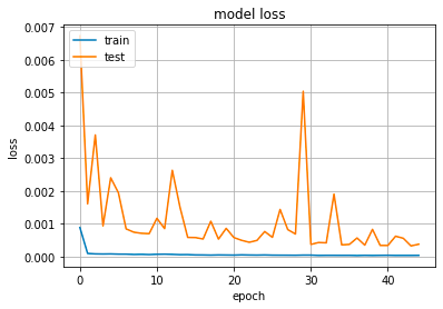 

This code displays the training progress of a machine learning model by plotting its loss over time. The graph shows the training validation loss on separate line graphs, with the x-axis representing the number of iterations the y-axis representing the loss value. The title, axis labels, legend are all set for clarity, the graph is displayed using a specific comm.

plt.plot(history.history['loss']) # t
plt.plot(history.history['val_loss'])
plt.title('model loss')
plt.ylabel('loss')
plt.xlabel('epoch')
plt.legend(['train', 'test'], loc='upper left')
plt.show() 

This code uses Python’s matplotlib library to graph the training process of a machine learning model. It shows the training validation loss over multiple epochs, with the training data being sourced from the history object’s history attribute. The title, axis labels, legend are included for clarity, the resulting plot is displayed using plt.show(). This visualization aids in evaluating the model’s performance detecting overfitting or underfitting.

plt.plot(history.history['loss']) # t
plt.plot(history.history['val_loss'])
plt.title('model loss')
plt.ylabel('loss')
plt.xlabel('epoch')
plt.legend(['train', 'test'], loc='upper left')
plt.show()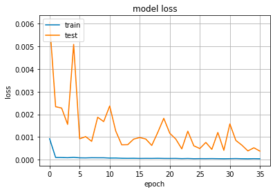 

The code uses the Matplotlib library to generate a graph showing the training validation loss of a machine learning model throughout its training process. The first plot comm displays the training loss, while the second comm, partially commented out, is supposed to show the validation loss. The graph’s title is set to ‘model loss’, with the y-axis labeled as ‘loss’ the x-axis as ‘epoch’. A legend, labeled ‘train’ ‘test’, is located in the top left of the graph. The code then displays the graph, allowing for the evaluation of the model’s learning potential overfitting or underfitting to the training dataset as the epochs progress.

train_predict=model.predict(X_train)
test_predict=model.predict(X_test)

In this code, a model is being used for predictions on two different datasets — the training dataset (X_train) the testing dataset (X_test). The first line records the model’s predictions for the training dataset in the variable train_predict, while the second line does the same for the testing dataset in test_predict. These predictions can be compared to the actual outcomes of both datasets to evaluate the model’s performance its ability to generalize.

train_predict=scaler.inverse_transform(train_predict)
test_predict=scaler.inverse_transform(test_predict)

In this code, a scaler object is used to convert scaled predictions back to their original scale for both training test data. This is necessary because the data may have been initially scaled down for machine learning modeling. The inverse_transform method is employed to reverse this scaling present the predictions in their original scale, allowing for better interpretation evaluation of the model’s performance.

import math
from sklearn.metrics import mean_squared_error
math.sqrt(mean_squared_error(y_train,train_predict))

This code snippet imports the math library for mathematical functions, the mean_squared_error function from the sklearn.metrics module of the scikit-learn library. It then uses the mean_squared_error function to calculate the average error between two sets of values, typically the true target values predicted values from a regression model. By taking the square root of this value, the root mean squared error (RMSE) is obtained, which is a commonly used metric to measure the performance of a regression model. A lower RMSE indicates a better fit between the model the data.

look_back=100
fig, ax = plt.subplots(figsize=(20,10))
trainPredictPlot = numpy.empty_like(y)
trainPredictPlot[:, :] = np.nan
trainPredictPlot[look_back:len(train_predict)+look_back, :] = train_predict
testPredictPlot = numpy.empty_like(y)
testPredictPlot[:, :] = numpy.nan
testPredictPlot[len(train_predict)+(look_back*2)+1:len(y)-1, :] = test_predict
plt.plot(scaler.inverse_transform(y))
plt.plot(trainPredictPlot)
plt.plot(testPredictPlot)
plt.legend(['inverse_transform(y)','trainPredictPlot','testPredictPlot'])
plt.xlabel('Time Steps')
plt.ylabel('Aaple Stock Price')
plt.show()

This Python code creates a plot to compare actual predicted stock prices for Apple. The plot is created step by step: 

1. A figure subplot are created with specific size dimensions. 

2. Two arrays with NaN values are initialized to match the shape of another array. 

3. A variable is defined to determine the number of previous data points to consider. 

4. Values from the training prediction array are added to one of the initial arrays, starting after the specified look-back period. 

5. Similarly, values from the testing prediction array are added to the other initial array, with an offset accounting for both training the look-back period. 

6. A line plot is created for the original stock prices, which have been reversed from a scaled representation to their original scale. 

7. Two more line plots are added for the training testing predictions. 

8. A legend is included to identify the different elements of the plot. 

9. Labels for the x-axis y-axis indicate time steps Apple stock prices. 

10. The plot is displayed to evaluate visually compare the predictive model’s performance on historical Apple stock prices for a training testing period.

look_back=100
fig, ax = plt.subplots(figsize=(20,10))
trainPredictPlot = numpy.empty_like(y)
trainPredictPlot[:, :] = np.nan
trainPredictPlot[look_back:len(train_predict)+look_back, :] = train_predict
testPredictPlot = numpy.empty_like(y)
testPredictPlot[:, :] = numpy.nan
testPredictPlot[len(train_predict)+(look_back*2)+1:len(y)-1, :] = test_predict
plt.plot(scaler.inverse_transform(y))
plt.plot(trainPredictPlot)
plt.plot(testPredictPlot)
plt.legend(['inverse_transform(y)','trainPredictPlot','testPredictPlot'])
plt.xlabel('Time Steps')
plt.ylabel('Aaple Stock Price')
plt.show()

This code visualizes the results of a forecasting model, such as predicting stock prices, by plotting the original series forecast on a chart. It uses a variable look_back to represent the number of previous time points considered in the prediction. The code creates a plot with specific dimensions, initializes an array with NaN values, updates it with predictions from the training test sets. The chart also includes an inverse transformation of the target data, legends to differentiate between actual predicted data, labels for the axes. By using plt.show(), users can visually compare the model’s predictions to the actual stock price trends for both sets.

train_mse = model.evaluate(X_train, y_train, verbose=1)
test_mse = model.evaluate(X_test, ytest, verbose=1)

This code This section describes different scenarios you might encounter when assessing the fit of your model:

1. Underfitting: This is characterized by high error rates in both training and validation phases. It indicates that the model is not capturing the underlying patterns in the data effectively.

2. Overfitting: In this case, you’ll observe that the validation error is high while the training error is low. This suggests that the model is too closely fitted to the training data and fails to generalize well to new, unseen data.

3. Good Fit: A model with a good fit is indicated by a low validation error, which is only slightly higher than the training error. This implies that the model has learned the patterns in the training data well and can generalize effectively to new data.

4. Unknown Fit: This scenario is a bit more complex, where the validation error is low, but the training error is high. It’s an unusual situation and might require a closer inspection to understand the model’s performance.

Each of these situations offers insights into how well your model is learning and generalizing from the given data.assesses the performance of a machine learning model, named ‘model’, on two datasets by calculating the Mean Squared Error (MSE) for the training test sets. The ‘verbose=1’ option shows progress logs, the results are stored in the ‘train_mse’ ‘test_mse’ variables. This helps determine how well the model performs on the training unseen data, informing decisions about its generalization ability.

Future Forecasting

temp_input=list(x_input)
temp_input=temp_input[0].tolist()

This snippet of code converts an input, x_input, into a list called temp_input. Next, it extracts the first element from this list, converts it to a regular Python list, reassigns it to temp_input. This element is presumed to be a complex data structure with the tolist() method, like a NumPy array.

from numpy import array

lst_output=[]
n_steps=100
i=0
while(i<30):
    
    if(len(temp_input)>100):
        x_input=np.array(temp_input[1:])
        print("{} day input {}".format(i,x_input))
        x_input=x_input.reshape(1,-1)
        x_input = x_input.reshape((1, n_steps, 1))
        yhat = model.predict(x_input, verbose=0)
        print("{} day output {}".format(i,yhat))
        temp_input.extend(yhat[0].tolist())
        temp_input=temp_input[1:]
        lst_output.extend(yhat.tolist())
        i=i+1
    else:
        x_input = x_input.reshape((1, n_steps,1))
        yhat = model.predict(x_input, verbose=0)
        print(yhat[0])
        temp_input.extend(yhat[0].tolist())
        print(len(temp_input))
        lst_output.extend(yhat.tolist())
        i=i+1

print(lst_output)

This code snippet is likely used in a time series forecasting script to make predictions using a pre-trained model. Initially, an empty list is created to store the predicted values, a loop is set up to generate 30 predictions. The code uses a sliding window approach with a window size of 100 to update the input data for each prediction. Inside the loop, the code checks if there are more than 100 data points in the most recent list, temp_input, removes the oldest point before making a prediction. The input data is then reshaped to fit the model’s expected structure, the model.predict() method is used to generate a prediction. The predicted value is printed added to the temp_input list, mimicking new data being received. If temp_input has 100 or fewer items, the list is reshaped, a prediction is made without trimming the list size. This process continues until 30 predictions are made, the resulting values are printed. Some details, such as the initialisation of temp_input, the model, import statements for model, are not shown in the code, assuming they are set up correctly elsewhere.

day_new=np.arange(1,101)
day_pred=np.arange(101,131)

This code snippet in Python uses the NumPy library to create two sets of numerical sequences. The first, named day_new, generates numbers starting from 1 to 100, while the second, day_pred, generates numbers from 101 to 130. However, this code may result in a syntax error due to missing separators between statements. It is assumed that the goal is to use NumPy’s arange function to create separate arrays.

plt.plot(day_new,scaler.inverse_transform(y[2880:]))
plt.plot(day_pred,scaler.inverse_transform(lst_output))

The code uses the plot function from the matplotlib library to create two line plots on one chart. It converts previously scaled data back to its original scale using a scaler object, plots one line for actual values another for predicted values over time.